Phenological Response of an Arizona Dryland Forest to Short-Term Climatic Extremes

Abstract

Baseline information about dryland forest phenology is necessary to accurately anticipate future ecosystem shifts. The overarching goal of our study was to investigate the variability of vegetation phenology across a dryland forest landscape in response to climate alterations. We analyzed the influence of site characteristics and climatic conditions on the phenological patterns of an Arizona, USA, ponderosa pine (Pinus ponderosa) forest during a five-year period (2005 to 2009) that encompassed extreme wet and dry precipitation regimes. We assembled 80 synthetic Landsat images by applying the spatial and temporal adaptive reflectance fusion method (STARFM) to 500 m MODIS and 30 m Landsat-5 Thematic Mapper (TM) data. We tested relationships between site characteristics and the timing of peak Normalized Difference Vegetation Index (NDVI) to assess the effect of climatic stress on the green-up of individual pixels during or after the summer monsoon. Our results show that drought-induced stress led to a fragmented phenological response that was highly dependent on microsite parameters, as both the spatial autocorrelation of peak timing and the number of significant site variables increased during the drought year. Pixels at lower elevations and with higher proportions of herbaceous vegetation were more likely to exhibit dynamic responses to changes in precipitation conditions. Our study demonstrates the complexity of responses within dryland forest ecosystems and highlights the need for standardized monitoring of phenology trends in these areas. The spatial and temporal variability of phenological signals may provide a quantitative solution to the problem of how to evaluate dryland land surface trends across time.

1. Introduction

1.1. Dryland Forests and Woodlands

Approximately one billion hectare of forests and woodlands exist within dryland areas around the globe [1]. One such forest ecosystem is found in the American Southwest, which hosts the largest expanse of pure ponderosa pine (Pinus ponderosa ex Laws.) forest in the world [2]. Dryland ecosystems are highly sensitive to climate variability [3,4]; even brief deviations from climatic norms can lead to rapid and persistent changes in the distribution of vegetation species [5]. The dry forest ecosystems of the U.S. West, particularly those dominated by ponderosa pine, were considered to be in “widespread collapse” over a decade ago [6] due to the interwoven dynamics of drought, forest mismanagement, and associated disturbance processes, such as pest infestations and fire. Between 1984 and 2008, an estimated 18% of Southwest forest areas suffered high levels of mortality from wildfires and bark beetles [7]. The frequency and extent of large wildfires, the length of the wildfire season, and the total area burned in western U.S. forests have all increased since the mid-1980s [8]. Recent bark beetle infestations are the largest in recorded history; pests and pathogens are expected to reduce U.S. ponderosa pine forests by 28% over the next 15 years (2013–2027), without taking into account the effects of climate change [9].

The near-term outlook for dryland forests in the American Southwest is not encouraging. Most climate models predict warming across the U.S. over the next century [10], with reduced water resource availability across the southwestern states [11]. Warming can exacerbate the physiological stress on dryland trees, resulting in higher rates of tree mortality and more frequent die-off events [12,13]. If the length and intensity of summer drought increases, the resulting increase in the frequency of large wildfires will likely lead to changes in forest composition and tree densities [8]. Forest area in the Southwest could be reduced or converted to non-forest by over 50% with only two more drought or die-off events that are on par with those in the recent past [7].

1.2. Ecological Importance of Dryland Forest Phenology

There is a pressing need to understand how dryland forests will react to climate change since these ecosystems provide a wide array of critical ecosystem services, ranging from nutrient cycling and wildlife habitats to timber harvesting and recreational opportunities [1]. Baseline information about the range of dryland forest responses to weather events is necessary to accurately predict ecological responses to climate change and its associated forcing agents [13,14]. The study of the timing and causes of recurrent biological events in a vegetative life cycle (e.g., “phenology” [15,16,17,18]) is a key element of global change studies [19]. Temperature and precipitation changes can alter the timing of plant development and senescence [18], which can profoundly affect climate-vegetation processes, such as land surface albedo, sensible and latent flux partitioning, the timing of photosynthesis, and the timing and amount of litterfall [19]. Increased wildfire activity in western U.S. forests, for instance, has been positively linked to the earlier occurrence of spring, as measured by the timing of snowmelt [8]. Phenological changes can, in turn, influence local climate conditions, forming feedback loops. Earlier spring green-up and delayed fall senescence in deciduous canopies have been shown to alter seasonal climate characteristics: the prolonged period of increased evapotranspiration lowered soil moisture, increased surface temperature, and ultimately reduced summer precipitation [20].

One complication is that the phenology of dryland ecosystems can be difficult to characterize and predict over landscape extents. Unlike deciduous ecosystems, in which vegetation dynamics are controlled primarily by temperature and photoperiod [21], drylands are typically governed by the timing and amount of precipitation [22,23]. The spatially scattered and temporally erratic precipitation in dryland ecosystems drives a heterogeneous distribution of phenology states across the landscape [24]. These patterns are difficult to characterize using standard phenology determination methods [25], which were developed to track the more predictable growth phases of temperate, deciduous ecosystems.

The vegetative composition and arrangement of ponderosa pine ecosystems exemplify this challenge. Historically, ponderosa pine ecosystems were composed of clumps of individual trees separated by inter-canopy expanses of herbaceous plants [26]. Fire suppression policies over the past century have generally led to denser, more evenly distributed stands of ponderosa pine, but the ecosystems can still display a wide array of vegetative compositions and structures arranged in a variety of mosaics [27]. The drought sensitivity of ponderosa pine is linked to landscape characteristics, such as elevation, slope, and soil texture [28,29], while increased tree density and lower elevation have been related to increased likelihood of mortality by bark beetles [26]. The removal of ponderosa pine overstory due to fire [30], insect infestations [26], and thinning [31] has been documented to stimulate the growth of understory forbs and grasses, which can produce different annual growth patterns than woody vegetation; herbaceous growth typically reacts quickly to precipitation and climatic events, while woody vegetation exhibits a measured and less dynamic response [32]. There is therefore a high potential for complex, localized patterns of phenology in ponderosa pine ecosystems.

1.3. Data Fusion for Remote Sensing of Dryland Phenology

Current satellite sensors are either temporally or spatially inadequate to capture the full phenological variability of dryland landscapes; infrequent revisit times may miss precipitous green-up events, while frequently-acquired but coarse-resolution data can aggregate multiple asynchronous signals into an incoherent response [25]. One solution to the lack of optimal imagery is to combine complementary data sources to overcome the inadequate temporal or spatial resolution of a single sensor. In this study we rely on the spatial and temporal adaptive reflectance fusion method (STARFM) [33]. This technique blends 500 m MODIS and 30 m Landsat imagery to produce “synthetic” imagery at MODIS time steps and 30 m resolution. Our earlier research established that STARFM can return accurate results in the dryland environment of Northern Central Arizona using Landsat-5 data, particularly when implemented with MODIS nadir-adjusted bidirectional reflectance data (NBAR) [34]. We additionally concluded that the studies of phenological patterns in ponderosa pine ecosystems would benefit from the analysis of a higher spatial and temporal resolution imagery dataset. Phenology profiles derived from a time series of STARFM imagery contained spatial and temporal details that were absent from parallel time series based on 500 m MODIS or lower temporal resolution Landsat data [34,35].

1.4. Objectives

In this study we applied STARFM data to the analysis of the phenological signatures exhibited by a dryland ponderosa pine ecosystem in Central Arizona. The analysis time frame (2005–2009) encompassed both anomalously wet and dry precipitation regimes. Our interest was in how general climate conditions, site characteristics, and vegetative composition modify the annual and multi-year expressions of phenological variability across the landscape. Consistent with the concept of “land surface phenology” (LSP) [36,37,38,39], our goal was to characterize the overall expressions of phenology across the landscape rather than to isolate the signals of a single representative vegetation species. Our specific objectives were to use a high spatial and temporal time series of imagery to:

(1)

Characterize the spatial and temporal variability of dryland forest phenology patterns in response to climate conditions;

(2)

Assess how terrain characteristics and vegetation composition influence the variability of phenological responses;

(3)

Investigate the use of phenological variability as an indicator of vegetation composition.

To our knowledge this study is one of the first to examine the vegetation growth dynamics of a dryland forest at a 16-day temporal and 30-m spatial resolution. Although the analysis time frame is too constrained to allow general conclusions about long-term phenological trends within the dryland forest study site, the project demonstrates the complexity and variability of phenology patterns displayed by these ecosystems.

2. Study Site and Data

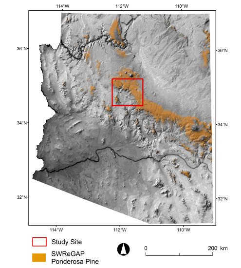
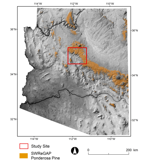
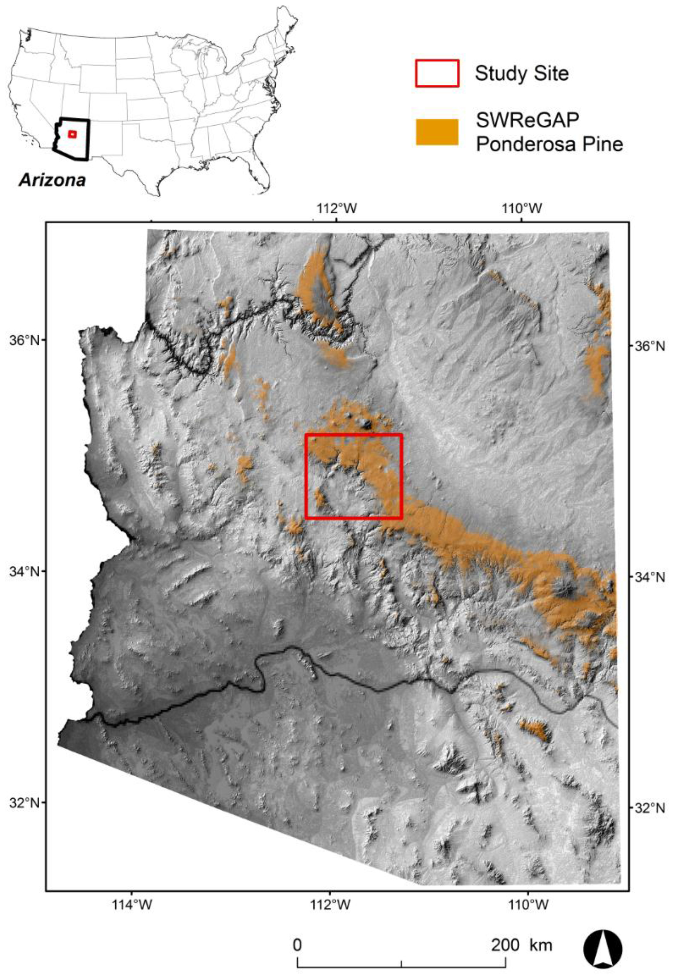
2.1. Study Site

The study area is the ponderosa pine forest ecosystem within a 7339 km² subset of Landsat WRS-2 path 37/row 36, centered at 34°53.5′N, 111°47.9′W in central Arizona (Figure 1). On average the area receives 364 mm of precipitation each year, primarily during the summer monsoon (July–early-September) and the winter months (November–March) [40,41] (Figure 2). The amount of precipitation received in 2005 was 117% of the annual average, while 2009 was anomalously dry (231 mm) due to the lack of monsoon activity. The precipitation amounts of the intervening years were closer to the 20th century annual mean, although the winter of 2006 (October 2005–February 2006) was the 3rd driest in the past century; only 40 mm of precipitation fell during that time, compared to an average of 147 mm [41].

Figure 1. Location of study area and extent of Southwest Regional Gap Analysis Program (SWReGAP) Southern Rocky Mountain Ponderosa Pine Woodland vegetation class in the state of Arizona, USA.

Figure 1. Location of study area and extent of Southwest Regional Gap Analysis Program (SWReGAP) Southern Rocky Mountain Ponderosa Pine Woodland vegetation class in the state of Arizona, USA.

Figure 2. Precipitation recorded in National Climatic Data Center (NCDC) Climate Division II in Arizona from 2005 to 2009, shown as (left) cumulative monthly totals, and (right) total monthly amounts.

Figure 2. Precipitation recorded in National Climatic Data Center (NCDC) Climate Division II in Arizona from 2005 to 2009, shown as (left) cumulative monthly totals, and (right) total monthly amounts.

2.2. Ponderosa Pine Land Cover

The vegetative ecosystem of interest is classified by the Southwest Regional Gap Analysis Program (SWReGAP) [42] as Southern Rocky Mountain Ponderosa Pine Woodland, which comprises the predominant land cover class in the study site. It is characterized by the dominance of ponderosa pine (Pinus ponderosa var. scopulorum and var. brachyptera) in the overstory. Douglas fir (Pseudotsuga menziesii), pinyon pine (Pinus edulis), and juniper (Pinus-Juniperus spp.) are also potentially found in the canopy, and a shrubby understory may be present. Commonly found associate grasses are bluebunch wheatgrass (Pseudoregneria spicata) and species of needlegrass (Achnatherum), grama (Bouteloua), fescue (Festuca), and muhly (Muhlenbergia) [43]. The ponderosa pine woodland is found at higher elevations in the study area (1945–2397 m).

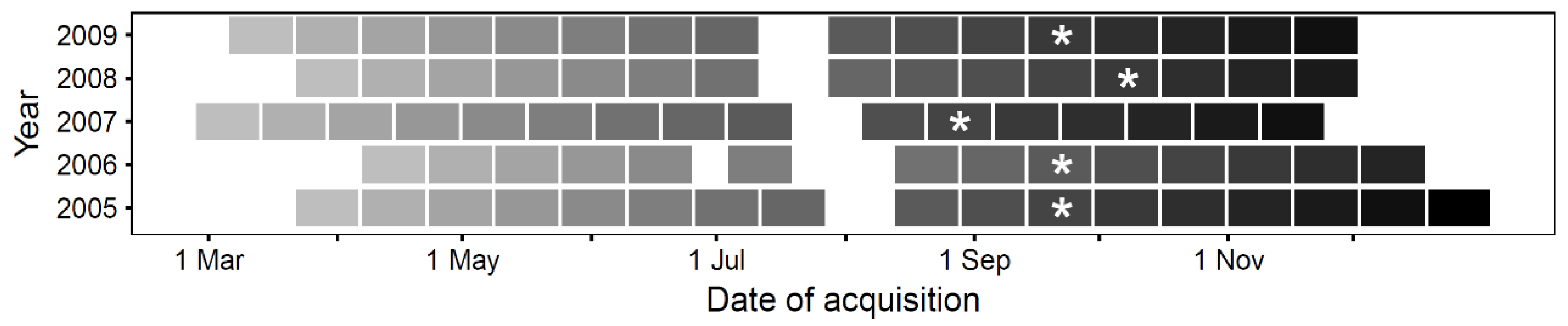
2.3. Imagery Datasets

2.3.1. MODIS

MODIS NBAR data (dataset MCD43A4) are produced every 8 days using 16 days of combined data from the Aqua and Terra satellites. The data use multi-angle surface reflectance values to model reflectances that would have been obtained from a nadir view given the mean solar zenith angle of the 16-day period [44,45,46].

We assembled MCD43A4 images acquired from 2005 to 2009 in tile h08v05, in which the quality control flags indicated no snow and full inversion for the bidirectional reflectance distribution function (BRDF) model for at least 95% of the study site. Although the 16-day datasets are output every 8 days, we used temporally adjacent 16-day datasets rather than including all available images. This restriction to non-overlapping datasets yields a more conservative time series and excludes potentially redundant information. At least 14 images met the criteria during the growing season in each year (Figure 3). The annual gap in the time series during the monsoon season does not invalidate the usefulness of the dataset for phenology analysis purposes [47].

Figure 3. Acquisition dates of 16-day MODIS NBAR datasets (MCD43A4). Gaps in the time series continuity were caused by cloud cover. Each MCD43A4 dataset identified with an asterisk (*) was combined with a contemporaneous Landsat image to create the annual STARFM base pair.

Figure 3. Acquisition dates of 16-day MODIS NBAR datasets (MCD43A4). Gaps in the time series continuity were caused by cloud cover. Each MCD43A4 dataset identified with an asterisk (*) was combined with a contemporaneous Landsat image to create the annual STARFM base pair.

We acquired all data via the Warehouse Inventory Search Tool (WIST) client at the USGS Earth Resources Observation and Science (EROS) Center website (https://lpdaac.usgs.gov). In accordance with the STARFM input requirements, the data were spatially subset to the study area dimensions, reprojected to a common projection (UTM Zone 12N), and resampled to a 30-m spatial resolution using a nearest neighbor transformation. We used the U.S. Geological Survey (USGS) MODIS Reprojection Tool (MRT v. 4.0) for all processing steps.

2.3.2. Landsat

In each year we chose a Landsat-5 Thematic Mapper (TM) image that was atmospherically clear (<5% cloud cover) and non-snowy as the basis for STARFM image generation. Given that our previous study returned favorable STARFM results based on fall scenes [34], we selected the clearest images available in that general time frame in each year: 16 September (2005); 19 September (2006); 21 August (2007); 10 October (2008); and 27 September (2009). We acquired all scenes through the USGS GLOVIS portal (http://glovis.usgs.gov), then calibrated and atmospherically corrected them using the Landsat Ecosystem Disturbance Adaptive Processing System (LEDAPS) [48]. The MODIS data processing scheme uses the same radiative transfer model for its atmospheric correction algorithm [48], thus, the use of LEDAPS for the Landsat correction decreases a potential source of uncertainty in the dataset comparison. No additional noise removal was required for the Landsat images from 2005, 2006, 2007, and 2009, while minor amounts of clouds and cloud shadows were masked from the 2008 image. Pixels with cloud cover in 2008 were removed from consideration in the overall study.

2.3.3. U.S. Department of Agriculture National Agriculture Imagery Program (NAIP) Imagery

We used 1-m NAIP imagery from May and June, 2011 to define percentages of overstory and understory cover at a set of random points across the study site, as outlined in Section 3.3.

2.4. Topographic Data

We downloaded individual 1/3 arc second (approximately 10 m) digital elevation model (DEM) files from the USGS National Elevation Dataset (NED) (http://ned.usgs.gov/). We mosaicked the study area files in ArcMap (v. 10.0; ESRI, Inc.) and resampled them to 30 m in ENVI (v.4.8) to conform to the STARFM data extent and resolution. We derived slope and aspect from the resampled DEM and subsequently partitioned the aspect data into eight, 45° sections: 1 (NNE: 0°–44°), 2 (NE: 45°–89°), 3 (SE: 90°–134°), 4 (SSE: 135°–179°), 5 (SSW: 180°–224°), 6 (SW: 225°–269°), 7 (NW: 270°–314°), and 8 (NNW: 315°–360°).

3. Methods

3.1. STARFM Algorithm

STARFM produces a synthetic image from one or more base pairs of Landsat and MODIS images acquired on the same day (t₀) and one or more MODIS observations from the prediction date (t₁). MODIS and Landsat surface data are very consistent relative to one another [48], although bandwidth and solar geometry differences cause variations [33]. After a MODIS surface reflectance image has been georeferenced and resampled to the same image size, pixel size, and coordinate system as the Landsat data, the high consistency of MODIS and Landsat surface reflectance data allows for the development of a stable relationship that can be extrapolated to subsequent MODIS images. The introduction of a weighting function adjusts reflectance values according to the complexity and heterogeneity of the study area. The resulting synthetic pixel values are quantitatively calibrated, rendering them useful for tracking changes in phenological metrics across time. Readers are referred to [33] for a thorough explanation of the algorithm.

We applied the STARFM algorithm to the assembled MODIS images, using a single imagery pair from each year, a moving window of 1500 × 1500 m, and band uncertainties of 0.002 and 0.005 for the visible and near infrared (NIR) bands, respectively [33]. In our previous studies, synthetic images generated from a single base pair returned acceptable results when compared to reference Landsat images acquired throughout the growing season [34,35]. We produced synthetic images corresponding to Landsat bands 3 (red) and 4 (NIR) only, for a total of 160 STARFM images (2 bands × 80 dates).

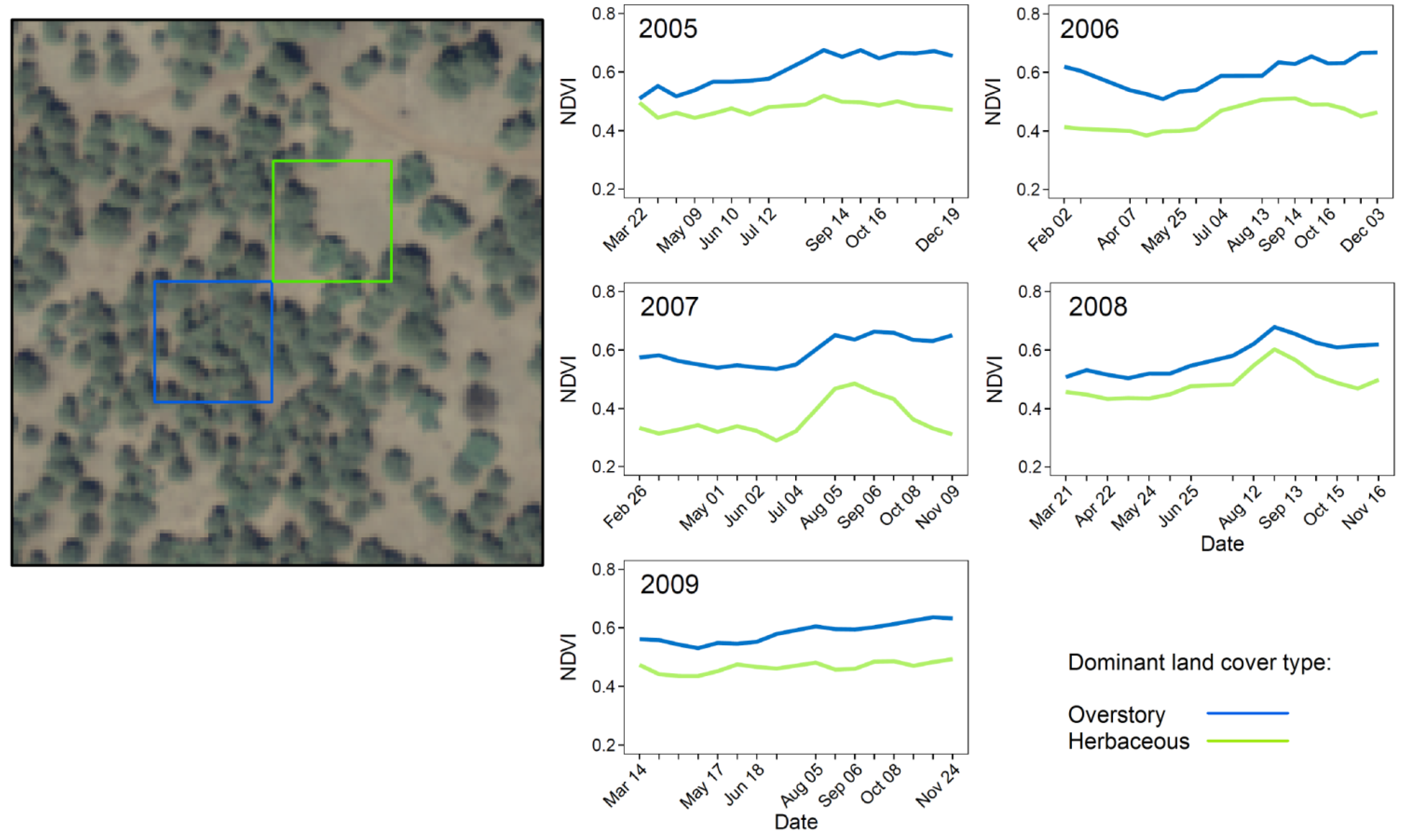
3.2. Creation of Time Series for Phenological Analysis

To examine the temporal signatures of the land cover classes, we extracted metrics derived from the Normalized Difference Vegetation Index (NDVI) [49]. NDVI is calculated as:

NDVI = (ρ_NIR – ρ_Red)/(ρ _NIR + ρ_Red)

(1)

where ρ indicates the reflectance of the associated band. We created NDVI images at each of the MODIS NBAR dates (Figure 3) to produce profiles of the vegetation dynamics during each growing season. We restricted the study to MODIS pixels in which all constituent 30 m STARFM pixels (typically ~240 pixels) were classified as Southern Rocky Mountain Ponderosa Pine Woodland (identified hereafter as “ponderosa pine”) in the SWReGAP dataset. This restriction reduced errors introduced by positioning discrepancies or classification inaccuracies, since adjacent pixels of the same land cover type are more likely to exhibit similar phenological behavior. A total of 1.3 million STARFM pixels met the criteria.

We extracted the annual reflectance time series profile from each 30-m pixel. Pixels with differing amounts of overstory or understory display profiles that diverge in both amplitude and timing; in most instances, neither type resembles the distinct seasonality trends that typify deciduous environments (Figure 4). We thus limited our analysis to a single key phenology metric: the timing of maximum greenness, i.e., the date of the maximum annual NDVI [50]. For each pixel we computed metrics for annual and multi-year (i.e., interannual) time periods. We computed all interannual parameters for both 2005–2008, to obtain a set of values representative of relatively average climatic conditions, and 2005–2009, to quantify the effect of the anomalously dry conditions of 2009 that substantially reduced regional NDVI values (Figure 5). T-tests of the mean peak NDVI value between the two groups (2005–2008: 0.57 vs. 0.56; t(1595.9) = 2.50, p = 0.01) and the date of peak NDVI (255.9 vs. 259.9; t(1587.8) = −3.33, p < 0.001) confirmed the distinctness of the classes.

Figure 4. Examples of seasonal differences in NDVI timing and value of herbaceous and woody vegetation. Shown are neighboring 30-m STARFM ponderosa pine land cover pixels dominated by overstory ponderosa pine (blue) or herbaceous vegetation (green). The background is 1-m resolution, natural-color U.S. Department of Agriculture (USDA) digital orthophoto quarter quad (DOQQ) imagery from June, 2007.

Figure 4. Examples of seasonal differences in NDVI timing and value of herbaceous and woody vegetation. Shown are neighboring 30-m STARFM ponderosa pine land cover pixels dominated by overstory ponderosa pine (blue) or herbaceous vegetation (green). The background is 1-m resolution, natural-color U.S. Department of Agriculture (USDA) digital orthophoto quarter quad (DOQQ) imagery from June, 2007.

Figure 5. Mean NDVI values of all ponderosa pine STARFM pixels from the contrasting precipitation years of 2005 (wet) and 2009 (dry). Error bars represent ± 1 one standard deviation. The effect of the lack of monsoon activity is evident in the 2009 profile, which diverges markedly from the 2005 response. To highlight the different vegetation dynamics between the years, the y-axis range has been reduced to (0.35, 0.65).

Figure 5. Mean NDVI values of all ponderosa pine STARFM pixels from the contrasting precipitation years of 2005 (wet) and 2009 (dry). Error bars represent ± 1 one standard deviation. The effect of the lack of monsoon activity is evident in the 2009 profile, which diverges markedly from the 2005 response. To highlight the different vegetation dynamics between the years, the y-axis range has been reduced to (0.35, 0.65).

3.3. Creation of Random Point Dataset

To evaluate the influence of topographic parameters and overstory proportion on phenology metrics, we generated a set of approximately 800 points located randomly across the STARFM ponderosa pine pixels. Areas that had burned during 2005–2009 were excluded to prevent disturbance events from affecting the phenology analysis. We visually estimated the percent of overstory cover within a 30-m square around each point on the basis of 1-m NAIP imagery hosted in Google Earth. We associated each point with multiple corresponding landscape and NDVI metrics, as well as the potential annual incident solar radiation [51] (Table 1, Figure 6). We included the mean NDVI as a covariate since this metric is associated with the relative proportion of pine or herbaceous material in each pixel, as demonstrated in Figure 4. Unlike the static percentage metric, however, the mean NDVI can vary from year to year. Information about how the timing and variability of NDVI response differ depending on annual mean NDVI is, thus, valuable for inferring how the seasonal dynamics change according to the relative greenness signal of each pixel.

Figure 6. Mean NDVI (top) and coefficient of variation (CV) of NDVI (bottom) of the 800 random points located within ponderosa pine STARFM pixels. Mean NDVI error bars represent ± 1 standard deviation.

Figure 6. Mean NDVI (top) and coefficient of variation (CV) of NDVI (bottom) of the 800 random points located within ponderosa pine STARFM pixels. Mean NDVI error bars represent ± 1 standard deviation.

Table 1. Mean and standard deviation (SD) descriptive statistics of variables in the annual and interannual analyses of peak NDVI timing. Values are calculated from the 800 random points located within ponderosa pine STARFM pixels. Mean NDVI and coefficient of variation (CV) of NDVI are shown in Figure 6.

Variables in Annual Analyses	Variables in Multi-Year Analyses	Mean (SD)
Elevation (m)	Elevation (m)	2158.65 (84.8)
Slope (°)	Slope (°)	4.50 (3.7)
Aspect (°)	Aspect (°)	211.17 (3.3)
Solar radiation (MJ/cm2/year)	Solar radiation (MJ/cm2/year)	0.99 (0.036)
Percent cover	Percent cover	48.89 (20.9)
	Peak NDVI value (2005 to 2008)	0.57 (0.064)
	Peak NDVI value (2005 to 2009)	0.56 (0.065)

Table 1. Mean and standard deviation (SD) descriptive statistics of variables in the annual and interannual analyses of peak NDVI timing. Values are calculated from the 800 random points located within ponderosa pine STARFM pixels. Mean NDVI and coefficient of variation (CV) of NDVI are shown in Figure 6.

Variables in Annual Analyses	Variables in Multi-Year Analyses	Mean (SD)
Elevation (m)	Elevation (m)	2158.65 (84.8)
Slope (°)	Slope (°)	4.50 (3.7)
Aspect (°)	Aspect (°)	211.17 (3.3)
Solar radiation (MJ/cm2/year)	Solar radiation (MJ/cm2/year)	0.99 (0.036)
Percent cover	Percent cover	48.89 (20.9)
	Peak NDVI value (2005 to 2008)	0.57 (0.064)
	Peak NDVI value (2005 to 2009)	0.56 (0.065)

4. Exploratory Data Analysis

Distribution plots of the peak timing of all ponderosa pine pixels revealed that the majority reaches peak greenness during or after the monsoon period. This distribution provided a convenient structure for assessing the broad influence of physical site characteristics and vegetative composition on peak timing. Our expectation was that a pixel that shows more immediate responsiveness to monsoonal precipitation is dominated by herbaceous cover, while one with a more delayed response is dominated by ponderosa pine, as demonstrated in other woody/herbaceous ecosystems (e.g., [32]). Pixels that alternate between monsoon and post-monsoon peaks likely have more equal vegetation distributions, either of which may dominate the annual signal depending on prevailing climate. As such, a study of the relative proportion of a landscape that greens up during or after the monsoon period may serve as a helpful measure of vegetative condition across broad extents. Our subsequent analytical goals were to evaluate the ability of the fused imagery time series to (1) discriminate the site characteristics that control the annual peak greenness timing (monsoon or post-monsoon); and (2) assess the consistency of the timing across the study time period.

4.1. Annual Patterns of Peak Greenness Timing

We chose a cut-off date of 15 October (Day of Year (DOY) 288) to distinguish between pre- and post-monsoon periods, based on the clear break in timing distributions in each year.

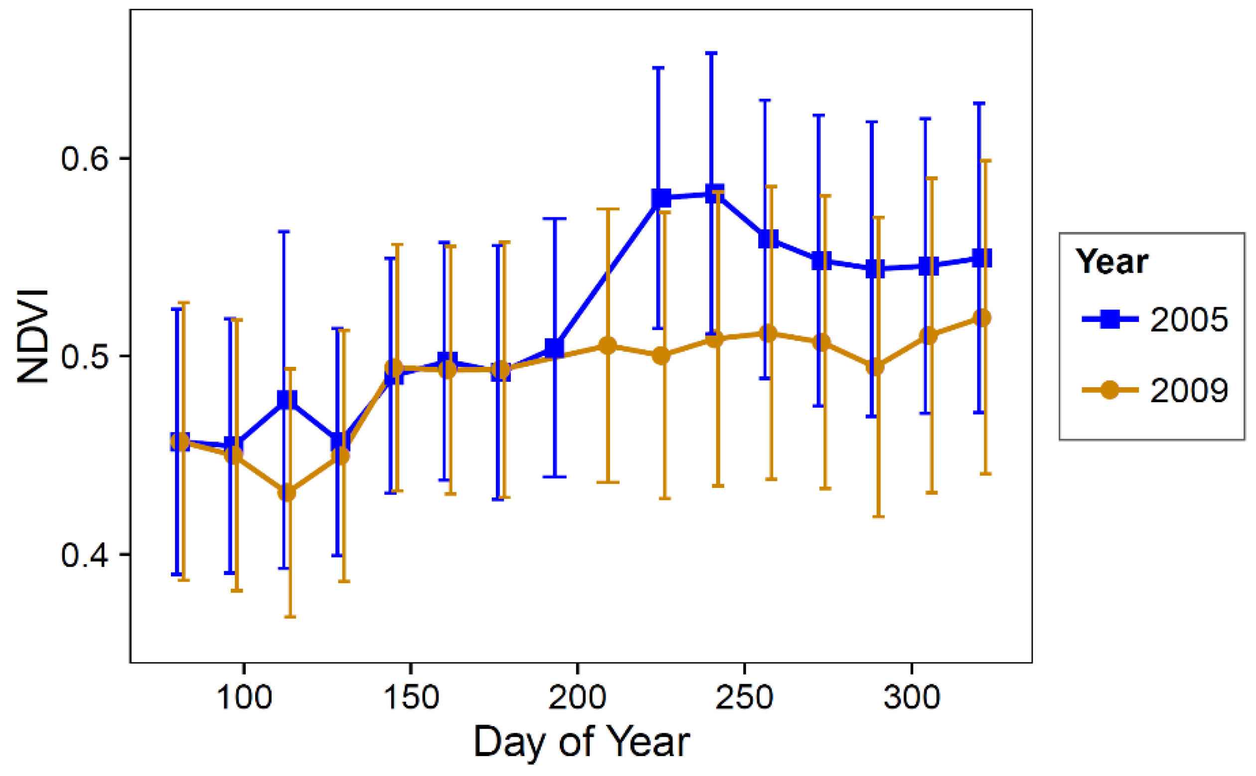
4.2. Interannual Patterns of Peak Greenness Timing

To determine whether each pixel displayed low or high variability of peak timing across years, we examined the standard deviation of peak NDVI timing for both 2005–2008 and 2005–2009. As in the annual analysis, distribution plots revealed bimodal distributions in each time frame. We fit individual Gaussian density components to each mixture distribution to distinguish between the two variability sets (Figure 7). To distinguish between low and high interannual variability groups, we chose the intersection of the two component density functions: 25 days for 2005–2008 and 20 days for 2005–2009.

Figure 7. Frequency distributions of the variation in peak NDVI date for 2005–2008 (left) and 2005–2009 (right). The time periods were analyzed separately to assess the behavior of high/average precipitation years vs. those that include a drought year (2009). Individual Gaussian functions are shown in blue (monsoon) and green (post-monsoon); the dashed line represents the density function for the composite distribution.

Figure 7. Frequency distributions of the variation in peak NDVI date for 2005–2008 (left) and 2005–2009 (right). The time periods were analyzed separately to assess the behavior of high/average precipitation years vs. those that include a drought year (2009). Individual Gaussian functions are shown in blue (monsoon) and green (post-monsoon); the dashed line represents the density function for the composite distribution.

5. Statistical Analysis

We explored the spatial and temporal patterns of the timing of peak greenness using a variety of statistical methods to determine whether landscapes that green up at different times—during or after the monsoon—exhibit different phenology signals under wet and dry conditions. Given that no available precipitation dataset in this region matches the high spatial resolution of our imagery dataset, we did not explicitly incorporate rainfall amount or timing into the analysis. Instead, we assume that the vegetation greenness patterns are primarily in response to the overall moisture conditions in each year.

5.1. Spatial Analysis

We investigated the degree to which climate affects the spatial distribution of peak greenness across the landscape by calculating the annual global Moran’s Index value [52] in ArcMap. Moran’s I can be thought of as the spatially-weighted equivalent of Pearson’s correlation coefficient [53], in which the null hypothesis assumes perfect homogeneity among the values. Thus a z-value of –1 indicates negative correlation (perfect dispersal); 0 indicates no correlation (random dispersion); and 1 indicates positive correlation (clustered). All 1.3 million ponderosa pine pixel values were included in this analysis in each year.

5.2. Comparison of Site Characteristics

To determine if vegetative and site characteristics differed between the respective annual (monsoon/post-monsoon greenup) and interannual groups (low/high variability of peak timing), we performed Welch’s t-tests for continuous variables, and chi-square tests and single-factor ANOVA and Tukey’s HSD (Honestly Significant Difference) tests for categorical aspect data. The random point dataset served as the basis for the examinations of site characteristics and model development to allow us to discriminate the behavior of pine- or herbaceous-dominated vegetation. All tests were conducted in R (version 2.14.1).

5.3. Multivariate Model Development and Analysis

To identify the multiple site and vegetation parameters that control when a pixel greens up and how variable that timing is over the five-year study period, we used a multiple logistic regression approach. In the annual analysis, the dependent binary variable was the green-up period to which a pixel belonged (monsoon or post-monsoon) and the independent variables were landscape parameters (elevation, slope, aspect, and solar), percent of overstory cover, and the annual mean and covariance of the NDVI value. In the interannual (multi-year) analysis, the dependent variable was the standard deviation group to which each pixel belonged (low or high), and the independent variables were the landscape parameters, percent of overstory cover, and the average peak NDVI value during 2005–2008 and 2005–2009. We used a backward stepwise model selection process with a combined bootstrap procedure to investigate the variability of model selection. The bootstrapping procedure strengthens the selection process accuracy by evaluating the distribution of each independent variable, which is used to distinguish between noise variables and true independent predictors [54]. The algorithm uses Akaike’s information criterion (AIC) as measure of the quality of the fit of the model.

6. Results

6.1. Test of Spatial Autocorrelation

The peak greenness dates showed positive spatial autocorrelation across the ponderosa pine landscape in all years except 2008 and a considerable range of magnitude (Table 2). The graphical presentation of the results (Figure 8) shows the predominance of monsoon timing in most years, with an abrupt change to highly clustered, post-monsoon timing in the anomalously dry year of 2009. Just 3.1% of all pixels registered a post-monsoonal peak NDVI in 2008, in contrast to 49.9% of all pixels in 2009.

Table 2. Results of the Moran’s I spatial correlation analysis of the annual date of peak NDVI in each year from 2005 to 2009. * p < 0.05. The data from all pixels were used in the analysis.

Year	Index	Z-Score	p
2005	0.40	2.83	0.005 *
2006	0.34	2.47	0.01 *
2007	0.38	2.73	0.006 *
2008	0.14	1.03	0.30
2009	0.86	6.11	<0.001 *

Table 2. Results of the Moran’s I spatial correlation analysis of the annual date of peak NDVI in each year from 2005 to 2009. * p < 0.05. The data from all pixels were used in the analysis.

Year	Index	Z-Score	p
2005	0.40	2.83	0.005 *
2006	0.34	2.47	0.01 *
2007	0.38	2.73	0.006 *
2008	0.14	1.03	0.30
2009	0.86	6.11	<0.001 *

Figure 8. Maps of the annual timing of peak NDVI recorded in each of the 1.3 million STARFM pixels from 2005 to 2009. Early-season pixels in 2007 (represented in blue) were excluded from the overall statistical analysis due to the presence of fire in that year.

Figure 8. Maps of the annual timing of peak NDVI recorded in each of the 1.3 million STARFM pixels from 2005 to 2009. Early-season pixels in 2007 (represented in blue) were excluded from the overall statistical analysis due to the presence of fire in that year.

6.2. Results of t-Tests and Logistic Regression of Annual Monsoon vs. Post-monsoon Timing Characteristics

The monsoon green-up group was consistently characterized by significantly lower amounts of overstory cover, lower mean NDVI, and higher coefficient of variation of NDVI, while topographic parameters were only significant in 2009 (elevation: 2179 m vs. 2144 m; t(648.93) = 5.61, p < 0.001; and slope: 5.01 vs. 4.14; t(657.58) = 3.27; p = 0.001) (Figure 9). Aspect and solar radiation were not significant in any year.

Figure 9. Results of Welch’s t-tests for landscape and vegetation parameters by monsoon or post-monsoon annual peak greenup in each year from 2005 to 2009 for 800 random point locations across the ponderosa pine ecosystem. Mean NDVI (top), coefficient of variation (CV) of NDVI (middle), and percent overstory cover (bottom) were significant at p < 0.05 in all years. Error bars in the mean NDVI and overstory cover plots represent +/− one standard error.

Figure 9. Results of Welch’s t-tests for landscape and vegetation parameters by monsoon or post-monsoon annual peak greenup in each year from 2005 to 2009 for 800 random point locations across the ponderosa pine ecosystem. Mean NDVI (top), coefficient of variation (CV) of NDVI (middle), and percent overstory cover (bottom) were significant at p < 0.05 in all years. Error bars in the mean NDVI and overstory cover plots represent +/− one standard error.

The logistic regression models run on a year-by-year basis revealed that as the mean NDVI value of a pixel increased, the probability of that pixel displaying a post-monsoon green-up also increased, while as the NDVI value variability increased, the probability dropped (Table 3). Shallower slopes were associated with higher probability of post-monsoon green-up in all years except 2008. Higher elevations corresponded to decreased probabilities of post-monsoon timing in the two drought years (2006 and 2009). Aspect was significant in 2006 only; the negative parameter coefficients on aspect partition 4 (135°–180°) indicate that the probability of post-monsoon timing decreased for vegetation in south/southeast-facing aspects.

Table 3. Results of the logistic regression modeling of the annual monsoon/post-monsoon timing of peak NDVI for 800 random point locations across the ponderosa pine ecosystem. SE = Standard error. * p < 0.05; ** p < 0.01; *** p < 0.001.

Year	Predictor	Coefficient	SE
2005	Intercept	−4.75 ***	1.05
	Slope	−0.062 *	0.028
	CV of NDVI	−0.25 ***	0.066
	Mean NDVI	11.26 ***	1.64
2006	Intercept	3.54	2.54
	Elevation	−0.004 **	0.001
	Slope	−0.08 ***	0.026
	CV of NDVI	−0.38 ***	0.060
	Mean NDVI	15.70 ***	0.06
	Aspect 4	−0.87 *	0.37
2007	Intercept	−2.83	1.77
	Slope	−0.15 **	0.050
	CV of NDVI	−0.53 ***	0.099
	Mean NDVI	10.29 **	2.73
2008	Intercept	−4.70 *	2.19
	CV of NDVI	−0.54 ***	0.13
	Mean NDVI	13.29 ***	3.43
2009	Intercept	14.96 *	2.31
	Elevation	−0.0059 ***	0.001
	Slope	−0.088 **	0.025
	CV of NDVI	−0.64 ***	0.066
	Mean NDVI	5.89 ***	1.41

Table 3. Results of the logistic regression modeling of the annual monsoon/post-monsoon timing of peak NDVI for 800 random point locations across the ponderosa pine ecosystem. SE = Standard error. * p < 0.05; ** p < 0.01; *** p < 0.001.

Year	Predictor	Coefficient	SE
2005	Intercept	−4.75 ***	1.05
	Slope	−0.062 *	0.028
	CV of NDVI	−0.25 ***	0.066
	Mean NDVI	11.26 ***	1.64
2006	Intercept	3.54	2.54
	Elevation	−0.004 **	0.001
	Slope	−0.08 ***	0.026
	CV of NDVI	−0.38 ***	0.060
	Mean NDVI	15.70 ***	0.06
	Aspect 4	−0.87 *	0.37
2007	Intercept	−2.83	1.77
	Slope	−0.15 **	0.050
	CV of NDVI	−0.53 ***	0.099
	Mean NDVI	10.29 **	2.73
2008	Intercept	−4.70 *	2.19
	CV of NDVI	−0.54 ***	0.13
	Mean NDVI	13.29 ***	3.43
2009	Intercept	14.96 *	2.31
	Elevation	−0.0059 ***	0.001
	Slope	−0.088 **	0.025
	CV of NDVI	−0.64 ***	0.066
	Mean NDVI	5.89 ***	1.41

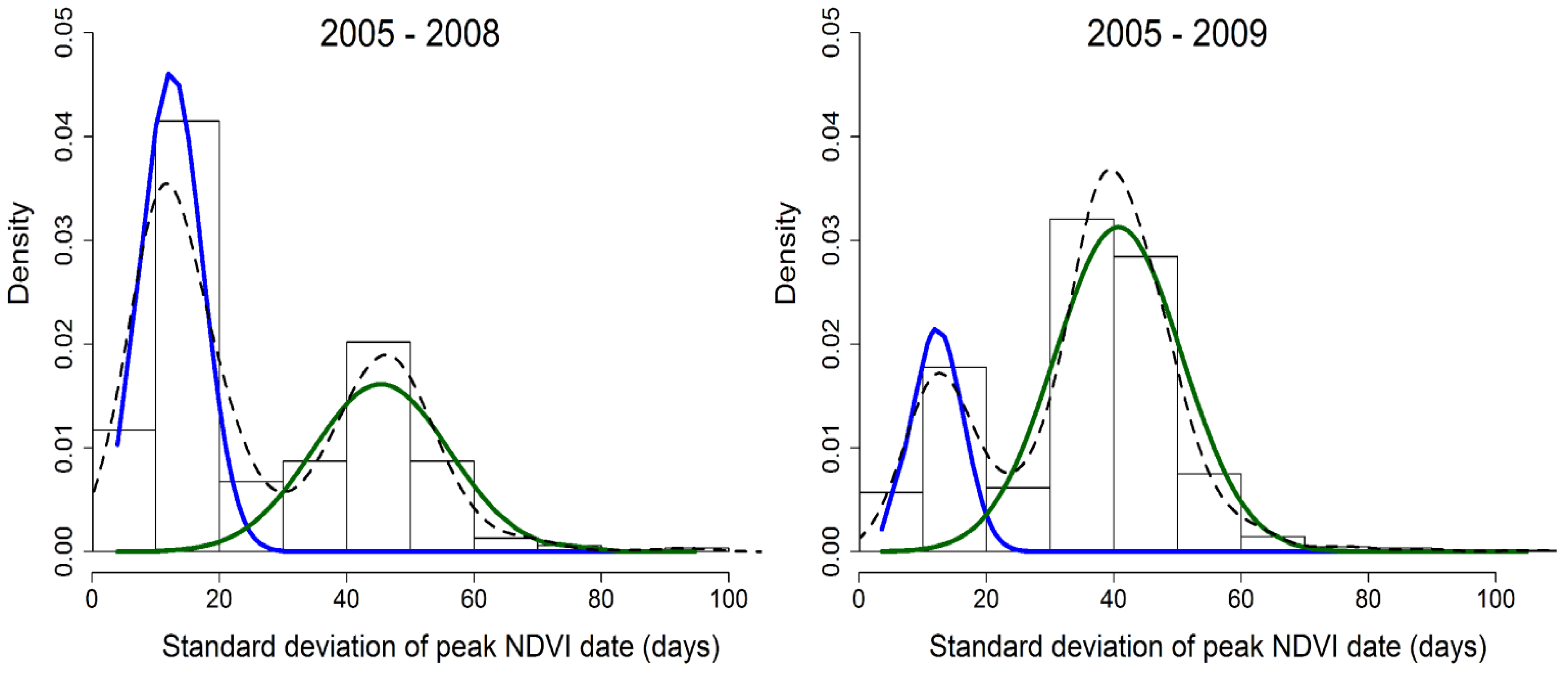
6.3. Results of t-Tests and Logistic Regression between Multi-Year Low vs. High Variability of Peak NDVI Date

Pixels with high variability from the average precipitation years of 2005–2008 were found at significantly lower elevations and displayed higher average peak NDVI values and higher percent overstory cover (Table 4). Pixels with high variability across both average and dry years were also found at lower elevations, with higher peak NDVI values; but they were conversely characterized by lower amounts of overstory cover, and located on significantly shallower slopes. The Chi-square analysis of the distribution of aspect categories could not reject the null hypothesis of no significant difference between high and low variability groups in both time periods (2005–2008: p = 0.09; 2005–2009: p = 0.54).

The logistic regression models for 2005–2008 and 2005–2009 reveal that only slope and elevation were significant factors influencing the variability of peak NDVI timing (Table 5). As either slope or elevation increased, the likelihood of a more consistent date of peak NDVI over time also increased. The mean peak NDVI value was a significant positive variable in 2005–2008, but was no longer significant when 2009 was included.

Table 4. Results of Welch’s t-test of variables in pixels displaying low or high variability of peak NDVI timing from 2005–2008 and 2005–2009 for 800 random point locations across the ponderosa pine ecosystem. Only parameters significant at p < 0.05 are shown. SD = standard deviation.

Time Period	Parameter	Variability of Peak NDVI Timing		T	df
		Low	High
		Mean (SD)	Mean (SD)
2005–2008	Elevation	2164.79 (90.97)	2149.87 (75.05)	2.53	775.74
	Percent cover	45.83 (20.48)	53.25 (20.63)	–5.02	702.84
	Mean peak NDVI	0.56 (0.064)	0.59 (0.059)	–7.06	739.89
2005–2009	Elevation	2183.95 (93.99)	2151.02 (80.70)	4.31	270.82
	Percent cover	51.62 (21.12)	48.06 (19.77)	2.11	320.89
	Mean peak NDVI	0.56 (0.059)	0.57 (0.066)	2.21	334.07
	Slope	5.30 (4.14)	4.27 (3.46)	3.06	266.03

Table 4. Results of Welch’s t-test of variables in pixels displaying low or high variability of peak NDVI timing from 2005–2008 and 2005–2009 for 800 random point locations across the ponderosa pine ecosystem. Only parameters significant at p < 0.05 are shown. SD = standard deviation.

Time Period	Parameter	Variability of Peak NDVI Timing		T	df
		Low	High
		Mean (SD)	Mean (SD)
2005–2008	Elevation	2164.79 (90.97)	2149.87 (75.05)	2.53	775.74
	Percent cover	45.83 (20.48)	53.25 (20.63)	–5.02	702.84
	Mean peak NDVI	0.56 (0.064)	0.59 (0.059)	–7.06	739.89
2005–2009	Elevation	2183.95 (93.99)	2151.02 (80.70)	4.31	270.82
	Percent cover	51.62 (21.12)	48.06 (19.77)	2.11	320.89
	Mean peak NDVI	0.56 (0.059)	0.57 (0.066)	2.21	334.07
	Slope	5.30 (4.14)	4.27 (3.46)	3.06	266.03

Table 5. Results of the logistic regression modeling of the low and high interannual variability of peak NDVI timing from 2005–2008 and 2005–2009 for 800 random point locations across the ponderosa pine ecosystem. * p < 0.05; *** p < 0.001.

Time period	Variable	Coefficient	SE
2005–2008	Intercept	0.59	4.18
	Elevation	–0.0031 ***	0.001
	Slope	–0.062 *	0.02
	Mean peak NDVI value	9.38 ***	1.72
2005–2009	Intercept	7.0	4.39
	Elevation	–0.0049 ***	0.001
	Slope	–0.052 *	0.02

Table 5. Results of the logistic regression modeling of the low and high interannual variability of peak NDVI timing from 2005–2008 and 2005–2009 for 800 random point locations across the ponderosa pine ecosystem. * p < 0.05; *** p < 0.001.

Time period	Variable	Coefficient	SE
2005–2008	Intercept	0.59	4.18
	Elevation	–0.0031 ***	0.001
	Slope	–0.062 *	0.02
	Mean peak NDVI value	9.38 ***	1.72
2005–2009	Intercept	7.0	4.39
	Elevation	–0.0049 ***	0.001
	Slope	–0.052 *	0.02

7. Discussion

As seen in other dryland ecosystems (e.g., [55]), the ponderosa pine forest ecosystem exhibited considerable phenological variability within seasons and across years during our study time period. This variability was consistently captured by the fused imagery time series, demonstrating that these data can be used to identify and quantify ecosystem response to climate conditions. We explore the ecological implications of the features captured by satellite data below.

7.1. Drought-Induced Stress Leads to Fragmented Phenological Response

The clustered response of 2009 peak NDVI timing to the marginal climate conditions (Figure 8) is likely the result of vegetation within neighborhoods of similar site characteristics exhibiting synchronized phenological responses; 49.9% of all pixels registered a post-monsoon peak NDVI. The obverse argument of less clustering across the landscape under wet or sufficiently rainy conditions, however, is less supported by these results; the most homogenous landscape was observed in a year of average precipitation (2008), in which just 3.1% of all pixels showed a post-monsoon peak NDVI, rather than during the extremely wet year (2005). Previous climate conditions may provide an explanatory context. Arizona experienced a severe drought prior to the start of our study period, from 2002–2004; tree-ring evidence implicates 2002 as the third-worst drought year in the last 1400 years [56]. The complex effects of antecedent climatic conditions on dryland system phenology [55] and the lagged influence of drought on subalpine tree species [57] may have influenced the 2005 response. In contrast, 2008 represents the first year of the time period that neither experienced seasonal drought (such as in 2006) nor was preceded by a drought year. The ecosystem may have recovered sufficiently at that point to permit a less fragmented response to climate conditions.

The average precipitation years of 2007 and 2008 also experienced different temperature regimes that might have contributed to the discrepancy in vegetation response. The average temperature from May through August 2007 (20.5 °C) was higher than the 20th century mean (19.0 °C), while the average temperature during the same time in 2008 was more moderate (19.3 °C) [41]. Although both years received approximately the same precipitation amount, the comparatively cooler conditions in 2008 may have been more amenable to vegetation growth.

7.2. Drought Intensifies the Discriminatory Power of Site Variables

During the drought year (2009), site characteristics became critical for determining the observed phenological response: post-monsoon pixels were found at significantly shallower slopes and lower elevations. This result appears inconsistent with the greater sensitivity of ponderosa pines to climate at lower elevations [28,29]. One explanation may be that the NDVI signal from pixels with relatively equal proportions of herbaceous and woody vegetation shifted to ponderosa pine-dominated timing at warmer, lower elevations due to a suppression of herbaceous response that did not occur at higher elevations. Supporting this explanation is the comparison of pixels that consistently experienced monsoon peaks from 2005 to 2009 with those that shifted from monsoon peak timing in wet or average precipitation years (2005–2008) to a post-monsoon peak in the dry year (2009). The stable monsoon vs. variable monsoon groups had no significant differences in percent cover (46% vs. 44%; t(430.46) = 0.78, p = 0.44), but displayed a significant effect for elevation (2182 m vs. 2141 m; t(435.41) = 4.87, p < 0.001), with inconsistent pixels found at lower elevations. Given the abbreviated time span of our study, we cannot draw conclusions about whether the signal shifts reflected a short-term seasonal response or a more permanent alteration of vegetation composition.

7.3. Variability of Peak NDVI Dates Linked to Topography and Herbaceous/Woody Composition

The variability of peak NDVI timing across moderate precipitation years (2005–2008) and moderate/drought years (2005–2009) demonstrates the influence of topographic factors and vegetative composition on the phenological response of the landscape to seasonal climate conditions.

The relatively narrow elevation range of our study site (452 m) played a prominent role in controlling phenological behavior, with lower elevations strongly linked to post-monsoon peaks and more variable peak green-up timing. Since we can regard elevation as a proxy for climate [58], the implication is that an examination of phenological response by stratified elevation gradients could be a useful tool for anticipating the effects of regional climate change [59].

All logistic regression models showed an association of shallower slopes with post-monsoon timing and more variable peak green-up dates. The higher variability of peak green-up from year to year is not consistent with a concurrent assumption of ponderosa pine-dominated pixels. We do not have an explanation for the dynamics of this particular scenario; the ponderosa pine may be responding to a critical deterministic factor that was not taken into account in this study, such as soil texture [29], species interactions, or resource availability.

The reversal of the association of higher peak NDVI timing variability with significantly greater percent cover (2005–2008) to significantly lower (2005–2009) may again reflect the suppression of herbaceous influence by the 2009 monsoon failure. Pixels with higher proportions of herbaceous vegetation were more likely to display a marked difference in peak greenness timing in response to the drought, as the dampened herbaceous signal allowed relatively smaller proportions of overstory cover to dominate. The amount of overstory cover never identified as a significant factor in the logistic regression modeling, despite its significance in the individual t-tests. Although percent cover was only moderately correlated with the annual average NDVI value and multi-year peak NDVI value, we suspect this collinearity was the reason that the parameter never evaluated as a significant factor.

8. Conclusions

Our study is unique in its investigation of the drivers of ponderosa pine ecosystem phenology using fused Landsat and MODIS data. We demonstrated that we could capture spatially complex phenology signals by examining changes in the seasonal timing of peak NDVI over a five-year span (2005–2009) that included extreme annual precipitation differences. Although a single metric cannot represent the full phenological complexity of this dryland environment, its behavior allows insights into how climate and site characteristics influence both broad and fine-scale patterns of vegetation dynamics.

Our results show that the 2009 drought produced more spatially and temporally unsynchronized signals of peak NDVI timing and shifted overall greenness patterns across the landscape: the percentage of all pixels with a post-monsoon peak NDVI increased from a low of 3.1% in the average precipitation year (2008) to a high of 49.9% during the drought year (2009). Drought additionally amplified the influence of microsite factors on vegetative response. In each year, selected pixels with monsoon peak greenness were characterized by significantly lower mean amounts of overstory cover (45.4%–48.4% vs. post-monsoon 50.7%–58.3%), lower mean annual NDVI (0.47–0.51 vs. 0.50–0.55), and higher annual NVDI coefficient of variation (7.9–10.6 vs. 6.0–8.9); in 2009, monsoon peak NDVI pixels were additionally found at higher mean elevations (2179 m vs. 2144 m) and steeper slopes (5.0 vs. 4.1). We further demonstrated that the consistency of peak NDVI timing was linked to the elevation and vegetation composition of each pixel. More stable peak green-up dates were uniformly associated with higher elevations (mean elevation difference: 23.9 m). However, consistent peak greenness timing alternated between an association with lower percent canopy cover in average and wet years (2005–2008; 45.8% vs. 53.3% for high-variability pixels) to an association with higher percent canopy when the drought year was included (2005–2009; 51.6% vs. 48.1%), demonstrating the complex response of the mixed woody and herbaceous ecosystem to extreme precipitation changes.

These results provide a basis for interpreting the phenological variability of dryland forests in terms of physical site parameters and woody/herbaceous vegetative composition. They also suggest that it may be time to reevaluate the defining characteristic of dryland vegetation dynamics: variability. Rather than viewing spatial and temporal variability as unwelcome noise that confounds standard ecological assessment techniques, we should explore its utility as an integral component of dryland vegetation dynamics. The degree, location, and patterns of variability can shed light on vegetative composition and functioning through time; a properly formulated synthesis metric may yield a quantitative solution to the question of how to evaluate land surface phenology trends across seasons and climatic conditions.

References and Notes

1. Safriel, U.; Adeel, Z.; Niemeijer, D.; Puigdefabregas, J.; White, R.; Lal, R.; Winslow, M.; Ziedler, J.; Prince, S.; Archer, E.; et al. Dryland systems. In Ecosystems and Human Well-Being: Current State and Trends (The Millennium Ecosystem Assessment Series); Hassan, R.M., Scholes, R., Ash, N., Eds.; Island Press: Washington, DC, USA, 2005; pp. 623–662. [Google Scholar]
2. Kaufmann, M.R.; Binkley, D.; Fulé, P.Z.; Johnson, M.; Stephens, S.L.; Swetnam, T.W. Defining old growth for fire-adapted forests of the western United States. Ecol. Soc. 2007, 12, 15. [Google Scholar]
3. Breshears, D.D.; Rich, P.M.; Barnes, F.J.; Campbell, K. Overstory-imposed heterogeneity in solar radiation and soil moisture in a semiarid woodland. Ecol. Appl. 1997, 7, 1201–1215. [Google Scholar] [CrossRef]
4. Hufkens, K.; Bogaert, J.; Dong, Q.H.; Lu, L.; Huang, C.L.; Ma, M.G.; Che, T.; Li, X.; Veroustraete, F.; Ceulemans, R. Impacts and uncertainties of upscaling of remote-sensing data validation for a semi-arid woodland. J. Arid Environ. 2008, 72, 1490–1505. [Google Scholar] [CrossRef]
5. Allen, C.D.; Breshears, D.D. Drought-induced shift of a forest-woodland ecotone: Rapid landscape response to climate variation. Proc. Natl. Acad. Sci. USA 1998, 95, 14839–14842. [Google Scholar] [CrossRef] [PubMed]
6. Covington, W.W. Helping western forests heal. Nature 2000, 408, 135–136. [Google Scholar] [CrossRef] [PubMed]
7. Williams, A.P.; Allen, C.D.; Millar, C.I.; Swetnam, T.W.; Michaelsen, J.; Still, C.J.; Leavitt, S.W. Forest responses to increasing aridity and warmth in the southwestern United States. Proc. Natl. Acad. Sci. USA 2010, 107, 21289–21294. [Google Scholar] [CrossRef] [PubMed]
8. Westerling, A.L.; Hidalgo, H.G.; Cayan, D.R.; Swetnam, T.W. Warming and earlier spring increase western U.S. forest wildfire activity. Science 2006, 313, 940–943. [Google Scholar] [CrossRef] [PubMed]
9. Krist, F.J., Jr.; Ellenwood, J.R.; Woods, M.E.; McMahan, A.J.; Cowardin, J.P.; Ryerson, D.E.; Sapio, F.J.; Zweifler, M.O.; Romero, S.A. 2013–2027 National Insect and Disease Forest Risk Assessment; Forest Health Technology Enterprise Team, United States Department of Agriculture, Forest Service: Washington, DC, USA, 2014. [Google Scholar]
10. Christensen, J.H.; Hewitson, B.; Busuioc, A.; Chen, A.; Gao, X.; Held, R.; Jones, R.; Kolli, R.K.; Kwon, W.K.; Laprise, R.; et al. Regional climate projections. In Climate Change 2007: The Physical Science Basis. Contribution of Working Group I to the Fourth Assessment Report of the Intergovernmental Panel on Climate Change; Solomon, S., Qin, D., Manning, M., Chen, Z., Marquis, M., Averyt, K.B., Tignor, M., Miller, H.I., Eds.; Cambridge University Press: New York, NY, USA, 2007; pp. 849–940. [Google Scholar]
11. Kirtman, B.; Power, S.B.; Adedoyin, J.A.; Boer, G.J.; Bojariu, R.; Camilloni, I.; Doblas-Reyes, F.J.; Fiore, A.M.; Kimoto, M.; Meehl, G.A.; et al. Near-term climate change: Projections and predictability. In Climate Change 2013: The Physical Science Basis. Contribution of Working Group I to the Fifth Assessment Report of the Intergovernmental Panel on Climate Change; Stocker, T.F., Qin, D., Plattner, G.-K., Tignor, M., Allen, S.K., Boschung, J., Nauels, A., Xia, Y., Bex, V., Midgley, P.M., Eds.; Cambridge University Press: Cambridge, UK, 2013; pp. 953–1028. [Google Scholar]
12. Adams, H.D.; Guardiola-Claramonte, M.; Barron-Gafford, G.A.; Villegas, J.C.; Breshears, D.D.; Zou, C.B.; Troch, P.A.; Huxman, T.E. Temperature sensitivity of drought-induced tree mortality portends increased regional die-off under global-change-type drought. Proc. Natl. Acad. Sci. USA 2009, 106, 7063–7066. [Google Scholar] [CrossRef] [PubMed]
13. Breshears, D.D.; Cobb, N.S.; Rich, P.M.; Price, K.P.; Allen, C.D.; Balice, R.G.; Romme, W.H.; Kastens, J.H.; Floyd, M.L.; Belnap, J.; et al. Regional vegetation die-off in response to global-change-type drought. Proc. Natl. Acad. Sci. USA 2005, 102, 15144–15148. [Google Scholar] [CrossRef] [PubMed]
14. Hicke, J.A.; Jenkins, J.C.; Ojima, D.S.; Ducey, M. Spatial patterns of forest characteristics in the Western United States derived from inventories. Ecol. Appl. 2007, 17, 2387–2402. [Google Scholar] [CrossRef] [PubMed]
15. Lieth, H. Phenology and Seasonality Modelling; Springer: Berlin, Germany, 1974. [Google Scholar]
16. Menzel, A. Trends in phenological phases in Europe between 1951 and 1996. Int. J. Biomet. 2000, 44, 76–81. [Google Scholar] [CrossRef]
17. Schwartz, M.D.; Ahas, R.; Aasa, A. Onset of spring starting earlier across the Northern Hemisphere. Global Chang. Biol. 2006, 12, 343–351. [Google Scholar] [CrossRef]
18. Cleland, E.E.; Chuine, I.; Menzel, A.; Mooney, H.A.; Schwartz, M.D. Shifting plant phenology in response to global change. Trends Ecol. Evol. 2007, 22, 357–365. [Google Scholar] [CrossRef] [PubMed]
19. White, M.A.; Brunsell, N.; Schwartz, M.D. Vegetation phenology in global change studies. In Phenology: An Integrative Environmental Science; Schwartz, M.D., Ed.; Kluwer Academic Publishers: New York, NY, USA, 2003; pp. 453–466. [Google Scholar]
20. Peñuelas, J.; Rutishauser, T.; Filella, I. Phenology feedbacks on climate change. Science 2009, 324, 887–888. [Google Scholar] [CrossRef] [PubMed]
21. Körner, C.; Basler, D. Phenology under global warming. Science 2010, 327, 1461–1462. [Google Scholar] [CrossRef] [PubMed]
22. Brown, J.H.; Valone, T.J.; Curtin, C.G. Reorganization of an arid ecosystem in response to recent climate change. Proc. Natl. Acad. Sci. USA 1997, 94, 9729–9733. [Google Scholar] [CrossRef] [PubMed]
23. Loik, M.E.; Breshears, D.D.; Lauenroth, W.K.; Belnap, J. A multi-scale perspective of water pulses in dryland ecosystems: Climatology and ecohydrology of the western USA. Oecologia 2004, 141, 269–281. [Google Scholar] [CrossRef] [PubMed]
24. Asner, G.P.; Borghi, C.E.; Ojeda, R.A. Desertification in central Argentina: Changes in ecosystem carbon and nitrogen from imaging spectroscopy. Ecol. Appl. 2003, 13, 629–648. [Google Scholar] [CrossRef]
25. White, M.A.; de Beurs, K.M.; Didan, K.; Inouye, D.W.; Richardson, A.D.; Jensen, O.P.; O’Keefe, J.; Zhang, G.; Nemani, R.R.; van Leeuwen, W.J.D.; et al. Intercomparison, interpretation, and assessment of spring phenology in North America estimated from remote sensing for 1982–2006. Global Chang. Biol. 2009, 15, 2335–2359. [Google Scholar] [CrossRef]
26. Negrón, J.F.; McMillin, J.D.; Anhold, J.A.; Coulson, D. Bark beetle-caused mortality in a drought-affected ponderosa pine landscape in Arizstona, USA. For. Ecol. Manag. 2009, 257, 1353–1362. [Google Scholar] [CrossRef]
27. Graham, R.T.; Jain, T.B. Ponderosa pine ecosystems. In Proceedings of the Symposium on Ponderosa Pine: Issues, Trends, and Management; Gen. Tech. Rep PSW-GTR-198; Pacific Southwest Research Station, U.S. Department of Agriculture, Forest Service: Berkeley, CA, USA, 2005; pp. 1–32. [Google Scholar]
28. Adams, H.D.; Kolb, T.E. Drought responses of conifers in ecotone forests of northern Arizona: Tree ring growth and leaf δ13C. Oecologia 2004, 140, 217–225. [Google Scholar] [CrossRef] [PubMed]
29. Knutson, K.C.; Pyke, D.A. Western juniper and ponderosa pine ecotonal climate-growth relationship across landscape gradients in southern Oregon. Can. J. For. Res. 2008, 38, 3021–3032. [Google Scholar] [CrossRef]
30. Bataineh, A.L.; Oswald, B.P.; Bataineh, M.M.; Williams, H.M.; Coble, D.W. Changes in understory vegetation of a ponderosa pine forest in northern Arizona 30 years after a wildfire. For. Ecol. Manag. 2006, 235, 283–294. [Google Scholar] [CrossRef]
31. Laughlin, D.C.; Bakker, J.D.; Daniels, M.L.; Moore, M.M.; Casey, C.A.; Springer, J.D. Restoring plant species diversity and community composition in a ponderosa pine-bunchgrass ecosystem. Plant Ecol. 2007, 197, 139–151. [Google Scholar] [CrossRef]
32. Rich, P.M.; Breshears, D.D.; White, A.B. Phenology of mixed woody-herbaceous ecosystems following extreme events: Net and differential responses. Ecology 2008, 89, 342–352. [Google Scholar] [CrossRef] [PubMed]
33. Gao, F.; Masek, J.; Schwaller, M.; Hall, F. On the blending of the Landsat and MODIS surface reflectance: Predicting daily Landsat surface reflectance. IEEE Trans. Geosci. Remote Sens. 2006, 44, 2207–2218. [Google Scholar]
34. Walker, J.J.; de Beurs, K.M.; Wynne, R.H.; Gao, F. Evaluation of Landsat and MODIS data fusion products for analysis of dryland forest phenology. Remote Sens. Environ. 2012, 117, 381–393. [Google Scholar] [CrossRef]
35. Walker, J.J.; de Beurs, K.M.; Wynne, R.H. Dryland vegetation phenology across an elevation gradient in Arizona, USA, investigated with fused MODIS and Landsat data. Remote Sens. Environ. 2014, 144, 85–97. [Google Scholar]
36. De Beurs, K.; Henebry, G.M. Land surface phenology, climatic variation, and institutional change: Analyzing agricultural land cover change in Kazakhstan. Remote Sens. Environ. 2004, 89, 497–509. [Google Scholar] [CrossRef]
37. Morisette, J.T.; Richardson, A.D.; Knapp, A.K.; Fisher, J.I.; Graham, E.A.; Abatzoglou, J.; Wilson, B.E.; Breshears, D.D.; Henebry, G.M.; Hanes, J.M.; et al. Tracking the rhythm of the season in the face of global change: phenological research in the 21st century. Front. Ecol. Environ. 2009, 7, 253–260. [Google Scholar] [CrossRef]
38. Ganguly, S.; Friedl, M.A.; Tan, B.; Zhang, X.; Verma, M. Land surface phenology from MODIS: Characterization of the Collection 5 global land cover dynamics product. Remote Sens. Environ. 2010, 114, 1805–1816. [Google Scholar] [CrossRef]
39. Henebry, G.M.; de Beurs, K.M. Remote sensing of land surface phenology: A prospectus. In Phenology: An Integrative Environmental Science; Schwartz, M.D., Ed.; Springer: New York, NY, USA, 2013; pp. 385–411. [Google Scholar]
40. Staudenmaier, M., Jr.; Preston, R.; Sorenson, P. Climate of Flagstaff, Arizona; NOAA Technical Document NWS WR-273; National Technical Information Service: Springfield, VA, USA, 2009. [Google Scholar]
41. National Oceanic and Atmospheric Administration (NOAA) National Climatic Data Center (NCDC) Climatological Rankings, 2005–2009. Available online: http://www.ncdc.noaa.gov/temp-and-precip/climatological-rankings/ (accessed on 15 January 2013).
42. Lowry, J.; Ramsey, R.D.; Thomas, K.; Schrupp, D.; Sajway, T.; Kirby, J.; Waller, E.; Schrader, S.; Falzarano, S.; Langs, L.; et al. Mapping moderate-scale land-cover over very large geographic areas within a collaborative framework: A case study of the Southwest Regional Gap Analysis Project (SWReGAP). Remote Sens. Environ. 2007, 108, 59–73. [Google Scholar] [CrossRef]
43. USGS National Gap Analysis Program. Southwest Regional GAP Analysis Project—Land Cover Descriptions; RS/GIS Laboratory, College of Natural Resources, Utah State University, 2005. Available online: http://earth.gis.usu.edu/swgap/data/atool/files/swgap_legend_desc.pdf (accessed on 21 March 2012).
44. Lucht, W. Expected retrieval accuracies of bidirectional reflectance and albedo from EOS-MODIS and MISR angular sampling. J. Geophys. Res.-Atmos. 1998, 103, 8763–8778. [Google Scholar] [CrossRef]
45. Lucht, W.; Schaaf, C.B.; Strahler, A.H. An algorithm for the retrieval of albedo from space using semiempirical BRDF models. IEEE Trans. Geosci. Remote Sens. 2000, 38, 977–998. [Google Scholar] [CrossRef]
46. Schaaf, C.B.; Gao, F.; Strahler, A.H.; Lucht, W.; Li, X.; Tsang, T.; Strugnell, N.C.; Zhang, X.; Jin, Y.; Muller, J.-P.; et al. First operational BRDF, albedo nadir reflectance products from MODIS. Remote Sens. Environ. 2002, 83, 135–148. [Google Scholar] [CrossRef]
47. Zhang, X.; Friedl, M.A.; Schaaf, C.B. Sensitivity of vegetation phenology detection to the temporal resolution of satellite data. Int. J. Remote Sens. 2009, 30, 2061–2074. [Google Scholar] [CrossRef]
48. Masek, J.G.; Vermote, E.F.; Saleous, N.E.; Wolfe, R.; Hall, F.G.; Huemmrich, K.F; Gao, F.; Kutler, J.; Lim, T.-K. A Landsat surface reflectance dataset for North America, 1990–2000. IEEE Geosci. Remote Sens. Lett. 2006, 3, 68–72. [Google Scholar] [CrossRef]
49. Tucker, C.J. A comparison of satellite sensor bands for vegetation monitoring. Photogramm. Eng. Remote Sens. 1978, 44, 1369–1380. [Google Scholar]
50. De Beurs, K.M.; Henebry, G.M. Spatio-temporal statistical methods for modelling land surface phenology. In Phenology of Ecosystem Processes: Applications in Global Change Research; Hudson, I.L., Keatley, M.R., Eds.; Springer: Dordrecht, The Netherlands, 2010; pp. 177–208. [Google Scholar]
51. McCune, B.; Keon, D. Equations for potential annual direct incident radiation and heat load. J. Veg. Sci. 2002, 13, 603–606. [Google Scholar] [CrossRef]
52. Moran, P.A.P. The interpretation of statistical maps. J. R. Stat. Soc. B 1948, 10, 243–251. [Google Scholar]
53. Goovaerts, P.; Jacquez, G.M.; Marcus, A. Geostatistical and local cluster analysis of high resolution hyperspectral imagery for detection of anomalies. Remote Sens. Environ. 2005, 95, 351–367. [Google Scholar] [CrossRef]
54. Austin, P.C.; Tu, J.V. Bootstrap methods for developing predictive models. Am. Stat. 2004, 58, 131–137. [Google Scholar] [CrossRef]
55. Jenerette, G.D.; Scott, R.L.; Huete, A.R. Functional differences between summer and winter season rain assessed with MODIS-derived phenology in a semi-arid region. J. Veg. Sci. 2010, 21, 16–30. [Google Scholar] [CrossRef]
56. Salzer, M.W.; Kipfmueller, K.F. Reconstructed temperature and precipitation on a millennial timescale from tree-rings in the southern Colorado Plateau, USA. Clim. Chang. 2005, 70, 465–487. [Google Scholar] [CrossRef]
57. Bigler, C.; Gavin, D.G.; Gunning, C.; Veblen, T.T. Drought induces lagged tree mortality in a subalpine forest in the Rocky Mountains. Oikos 2007, 116, 1983–1994. [Google Scholar] [CrossRef]
58. Davison, J.E.; Breshears, D.D.; van Leeuwen, W.J.D.; Casady, G.M. Remotely sensed vegetation phenology and productivity along a climatic gradient: On the value of incorporating the dimension of woody plant cover. Global Ecol. Biogeogr. 2011, 20, 101–113. [Google Scholar] [CrossRef]
59. Hudson Dunn, A; de Beurs, K.M. Land surface phenology of North American mountain environments using moderate resolution imaging spectroradiometer data. Remote Sens. Environ. 2011, 115, 1220–1233. [Google Scholar]