Using Simplified Thermal Inertia to Determine the Theoretical Dry Line in Feature Space for Evapotranspiration Retrieval

Abstract

With the development of quantitative remote sensing, regional evapotranspiration (ET) modeling based on the feature space has made substantial progress. Among those feature space based evapotranspiration models, accurate determination of the dry/wet lines remains a challenging task. This paper reports the development of a new model, named DDTI (Determination of Dry line by Thermal Inertia), which determines the theoretical dry line based on the relationship between the thermal inertia and the soil moisture. The Simplified Thermal Inertia value estimated in the North China Plain is consistent with the value measured in the laboratory. Three evaluation methods, which are based on the comparison of the locations of the theoretical dry line determined by two models (DDTI model and the heat energy balance model), the comparison of ET results, and the comparison of the evaporative fraction between the estimates from the two models and the in situ measurements, were used to assess the performance of the new model DDTI. The location of the theoretical dry line determined by DDTI is more reasonable than that determined by the heat energy balance model. ET estimated from DDTI has an RMSE (Root Mean Square Error) of 56.77 W/m² and a bias of 27.17 W/m²; while the heat energy balance model estimated ET with an RMSE of 83.36 W/m² and a bias of −38.42 W/m². When comparing the coeffcient of determination for the two models with the observations from Yucheng, DDTI demonstrated ET with an R² of 0.9065; while the heat energy balance model has an R² of 0.7729. When compared with the in situ measurements of evaporative fraction (EF) at Yucheng Experimental Station, the ET model based on DDTI reproduces the pixel scale EF with an RMSE of 0.149, much lower than that based on the heat energy balance model which has an RMSE of 0.220. Also, the EF bias between the DDTI model and the in situ measurements is 0.064, lower than the EF bias of the heat energy balance model, which is 0.084.

1. Introduction

Evapotranspiration (ET) monitoring has important implications in many aspects, such as improving regional and global climate models, understanding the hydrological cycle, and assessing environmental stress on natural and agricultural ecosystems [1,2]. With the development of remote sensing technology, estimating regional ET has made great progresses [3,4,5,6]. Satellite-based ET modeling can be categorized into one-layer schemes and two-layer schemes. Examples of the one-layer scheme include the Surface Energy Balance Algorithm (SEBAL) [7], the Surface Energy Balance (SEBS) [8], and the Simplified Surface Energy Balance Index (S-SEBI) [9]. Some representative two-layer models are N95 [10], the two-source energy balance approach [11], and the operational two-layer remote sensing model [12]. In the one-layer model, a mixed pixel composed of vegetation and soil is treated as a block. These one-layer models are suitable for regions with homogeneous dense vegetation or bare soil, but in many regions, such as semi-arid regions where patches of vegetation and bare soil are mixed, two-layer models perform much better than one-layer models. Two-layer models can estimate evaporation from soil and transpiration from vegetation separately, which is an important progress in the ET modeling. In the two-layer model, separating vegetation temperature and soil temperature is the most important procedure. One model to separate temperatures is to use the Priestly-Taylor factor, proposed by Norman [10]. This model estimates evapotranspiration and the vegetation temperature by using the Priestly-Taylor factor first; then, the soil temperature can be estimated from the land surface temperature, vegetation cover fraction, and vegetation temperature. However, determining an optimal value for the Priestly-Taylor factor is quite challenging in this model. Norman first chose a value of 1.3, then Kustas and Norman changed the Priestly-Taylor factor to 2 [13]. Later, Xu reported that 1.26 was more reasonable in wet areas [14]. Another model to separate temperature, named Pixel Component Arranging and Comparing Algorithm (PCACA), was proposed by Zhang and separates temperatures based on the hypothesis of a linear mixing structure of vegetation and soil in a pixel [12].

The third model to retrieve evapotranspiration is based directly on the relationship between the vegetation index and the land surface temperature and is known as the feature space model [4,15,16,17,18,19]. The advantage of using the feature space model is that complex parameterization of aerodynamic and surface resistances for water and heat transfer can be avoided; meanwhile, the feature space of VFC_LST (vegetation fraction cover versus land surface temperature) is able to capture the availability of soil moisture essential for evapotranspiration. The feature space model has been used widely by the remote sensing community. As Carlson has noted, that when a large number of pixels exist in the study area and exceptional pixels are removed, a triangular shape exists in the feature space [20]. In order to apply the CWSI (Crop Water Stress Index) to partially-vegetated fields, Moran proposed a Vegetation Index/Temperature (VIT) trapezoid model [16].

The location of the dry/wet line within the feature space directly affects the performance of the space feature model. The theoretical dry line corresponds to the pixels with the largest water stress and zero ET. The theoretical wet line corresponds to the pixels without any water stress and ET is close to the potential evapotranspiration. In previous studies, the wet line was usually determined by the lowest land surface temperature in the image, air temperature or by the temperature of nearby bodies of water. The dry line, though, is more difficult to determine due to the existence of abnormal or false dry pixels. Tang presented an iterative algorithm to automatically determine the dry line [21]. The algorithm, firstly, segments the whole fractional vegetation cover region into M bins; secondly, the abnormal pixels are removed according to the mean value and standard deviation of each bin; thirdly, the highest values in each bin are chosen as values to determine the dry line; finally, the dry line is determined by a linear regression of the highest values. Tang’s model can determine the dry line quickly, but for wet areas, such as after a rainfall, the dry line obtained is not the “true” theoretical dry line because dry pixels are not available.

An evapotranspiration model named the two-layer remote sensing model was proposed first by Zhang [12] and was then optimized by Zhang in 2008 [20]. In this model, the positions of the theoretical dry line and the theoretical wet line (especially the dry line) are key parameters. Zhang’s model is based on the heat energy balance model, and air temperatures are used to calculate the sensible heat flux. Air temperature data are obtained from nearby weather stations. This model can determine the theoretical dry line, but in wet weather, the dry line determined is not the true theoretical dry line because air temperatures are obtained from wet cases. The model based on the heat energy balance equation is called the heat energy balance model in this article. This model will be discussed in detail in Section 2.

Since there is insufficient study on the determination of the theoretical dry line’s location, this paper proposes a new model based on thermal inertia to obtain the theoretical dry line in the feature space, and it will be compared with the heat energy balance model using the same data set in order to provide an insight into the performance of two models. Section 2 presents the methodology of both the new model (DDTI) and the heat energy balance model. Experimentation results and a laboratory evaluation of the thermal inertia are shown in Section 3, followed by an application of the DDTI model in Section 4. The discussion is provided in Section 5. Finally, conclusions are given in Section 6.

2. Methodology

2.1. The Heat Energy Balance Model

In the two-layer remote sensing model [20], there are three main procedures in the ET estimation: The first is the PCACA model to decompose the temperature of the mixed pixels; the second is to determine the location of the theoretical dry and wet lines by heat energy balance equations; the third is the layered energy-separating algorithm to determine the Bowen Ratio. The detailed description of the three procedures can be found in Zhang (2008) [20].We focus on how to determine the theoretical dry line in this paper. For pixels on the theoretical dry line, ET is assumed to be 0. Based on the heat energy balance equation and ignoring advection in the horizontal direction, Equation (1) can be derived

$$R_n-G=H$$

(1)

where R_n is the net radiation, G is soil heat flux, and H is the sensible heat flux.

According to the empirical correlation between soil heat flux and the net radiation, G can be estimated by Equation (2) [22].

$$G=C{R}_n$$

(2)

when LST is greater than 275.15 K, $C=\left(LST-273.15\right)\left(0.0038+0.007a\right)\left(1-0.98NDV{I}^4\right)$. LST is the land surface temperature (K), $a$ is the surface albedo, NDVI is Normalized Difference Vegetation Index. When LST is less than or equal to 273.15 K, $C=0.35\times \left(1-f\right)$, and f is the vegetation fraction cover (VFC) [23].

The sensible heat flux and the net radiation can be estimated by Equations (3) and (4), respectively.

$$H=\frac{\text{ρ}{C}_p\left(T_{sd}-T_{sda}\right)}{r_{sda}}$$

(3)

$$R_n=S_0\left(1-{\text{α}}_{sd}\right)+{\text{σε}}_{sky}{T}_{sky}^4-\text{σ}{e}_{sd}{T}_{sd}^4$$

(4)

The temperature of the theoretical dry bare soil surface in Equation (5) can be deduced from Equations (1) to (4).

$$T_{sd}=\frac{\left(1-C\right)\left[S_0\left(1-{\text{α}}_{sd}\right)+{\text{σε}}_{sky}{T}_{sky}^4\right]+\frac{\text{ρ}{C}_p}{r_{sda}}{T}_{sda}}{\frac{\text{ρ}{C}_p}{r_{sda}}+\left(1-C\right){\text{σε}}_{sd}{T}_{sd}^3}$$

(5)

$$T_{vd}=\frac{\left(1-C\right)\left[S_0\left(1-{\text{α}}_{vd}\right)+{\text{σε}}_{sky}{T}_{sky}^4\right]+\frac{\text{ρ}{C}_p}{r_{vda}}{T}_{vda}}{\frac{\text{ρ}{C}_p}{r_{vda}}+\left(1-C\right){\text{σε}}_{vd}{T}_{vd}^3}$$

(6)

In the same way, the temperature of a theoretical dry surface with a full vegetation cover can be described by Equation (6). In the above equations, T_sd and T_vd are the surface temperatures of the two endpoints on the theoretical dry line (Figure 1), ρ is density of air, C_p is the volumetric heat capacity of air, r_sda and r_vda are the aerodynamic resistance, ε_sd and ε_vd are the emissivity of bare soil area and full vegetation coverage, $\text{σ}$ is the Stefan-Boltzmann Constant, S_o is the total solar incident radiation, α_sd and α_vd are the albedo of dry bare soil and full vegetation coverage, ε_sky is the emissivity of the sky, T_sda and T_vda are the air temperatures above the bare soil area and the full cover vegetation area, respectively.

Figure 1. Schematic figure of the theoretical dry line in the feature space of temperature (in K) and VFC.

Figure 1. Schematic figure of the theoretical dry line in the feature space of temperature (in K) and VFC.

2.2. The Thermal Inertia Model

In physics, thermal inertia is defined as Equation (7) [24].

$$P=\sqrt{K{\text{ρ}}_{s}c }$$

(7)

where P is the thermal inertia in J·m⁻²·K⁻¹·S^−1/2, K is the thermal conductivity in J·m⁻²·K⁻¹·S^−1/2, ρ_s is the density in gm⁻³, and c is the specific heat capacity in J·m⁻²·K⁻¹. For wet soil, based on the linear mixture model, its thermal inertia can be described by Equation (8) [25].

$$P_{ws}=\frac{V_s{P}_s+V_w{P}_w}{V_s+V_w}$$

(8)

where P_ws, P_s, and P_w are thermal inertia for wet soil, dry soil, and water, respectively. V_s and V_w are the volumetric proportions of soil and water in a soil sample. For the dry soil with minimal water content, its thermal inertia depends on soil type and structure. Thermal inertia for dry soil will remain the same if its type and structure do not change. For dry soil, thermal inertia represents the resistance to change in the temperature of the upper few centimeters of the surface throughout the day, and it is independent of the local time, latitude, and the season [26].

Due to the fact that thermal conductivity, density, and specific heat capacity cannot be measured in the field at a regional scale, it restricts greatly the application of thermal inertia. In 1977, Price derived the approximate analytical solution of thermal inertia by solving the thermal conducting equation, which is shown in Equation (9) [27].

$$P\approx \frac{2J}{{\text{ω}}^{\frac{1}{2}}\left(T_{max}-T_{min}\right)}$$

(9)

where P is thermal inertia ($\text{Cal}\cdot S^{-\frac{1}{2}}\cdot {℃}^{-1}\cdot c{m}^{-2}$); J is the incident net flux; ω is measurement cycle; T_max and T_min are the extremes of temperature response of the surface to the incident flux. Since then, thermal inertia can be estimated by incident flux, the increment of surface temperature and time of duration. Due to the three parameters can be obtained by remote sensing method in large area, thermal inertia has been applied widely in geography, such as discriminating categories of rock and soil moisture estimating [28,29,30,31,32,33,34].

Another thermal inertia, apparent thermal inertia (ATI), which is a mission product in determining surface characteristics from the heat Capacity Mapping Mission (HCMM) [24], is defined as

$$\begin{gathered} ATI=1000\pi \times \frac{\left(1-\text{α}\right)C_1}{T\left(1:30p.m.\right)-T\left(2:30p.m.\right)} \\ {\text{C}}_1=\left(\raisebox{1ex}{$1$}\!\left/ \!\raisebox{-1ex}{$\text{π}$}\right.\right)\left[\sin \text{δ}\sin \varnothing {\left(1-\tan {\text{δ}}^2\tan {\varnothing }^2\right)}^{\raisebox{1ex}{$1$}\!\left/ \!\raisebox{-1ex}{$2$}\right.}+\text{x}\cos \text{δ}\cos \varnothing \right] \end{gathered}$$

(10)

where α is the surface albedo, δ is the solar declination, $\varnothing$ is the latitude of observation. The incident flux is not include in the Equation (10) and its dimension is 1/°C It was reported that apparent thermal inertia should not be used in regions having variability in surface moisture [24].

In this paper, we use a new thermal inertia concept, simplified thermal inertia (STI), defined in Equation (11). The net radiation can be estimated by remote sensing methods with a high accuracy and we assume that net radiation increase linear from early morning to noon; therefore, the net radiation is used to calculate the thermal inertia.

$$P_s=\frac{\overline{R_{ns}}\sqrt{\left(t_2-t_1\right)}}{T_{s2}-T_{s1}}$$

(11)

where P_s is the STI for soil, t₁ and t₂ are the start and end times of the measurements, T_s1 and T_s2, are the soil surface temperatures at t₁ and t_2, and $\overline{R_{ns}}$ is the mean net radiation from t₁ to t₂.

According to the above definition, the simplified thermal inertia for dry soil can be estimated from an extremely dry situation in a historical period. For example, the thermal inertia value P_sd of a historical dry situation can be calculated by Equation (12). Then, P_sd can be used in a wet situation in Equation (13) in order to derive the temperatures on the theoretical dry line. T_s2h is the theoretical dry temperature.

$$P_{sd}=\frac{\overline{R_{nsd}}\sqrt{t_{2d}-t_{1d}}}{T_{s2d}-T_{s1d}}$$

(12)

$$T_{s2h}=\frac{\overline{ R_{nsh}}\sqrt{t_{2h}-t_{1h}}}{P_{sd}}+T_{s1h}$$

(13)

where t_1d and t_2d are the start and end times of the measurements in a dry situation. T_s1d and T_s2d are the soil surface temperatures at t_1d and t_2d, $\overline{R_{nsd}}$ is the mean net radiation from time t_1d to time t_2d, t_1h and t_2h are the start and end times of measurements in a wet situation, T_s1h and T_s2h are the soil surface temperatures at t_1h and t_2h, and $\overline{R_{nsh}}$ is the mean net radiation from time t_1h to t_2h.

In Equation (13), all of the variables on the right-hand side except P_sd are observed in a wet situation. In this paper, the model for calculating the simplified thermal inertia P_sd from a dry situation that is then used in a wet situation is called DDTI (Determination of Dry line by Thermal Inertia)

As is known, soil thermal inertia cannot be estimated by remote sensing in vegetation covered areas [24]. Although the mechanism of determining surface temperature change of vegetation is quite different from the mechanism of determining the surface temperature change of soil, the diurnal cycle of vegetation surface temperature is quite similar to that of soil. Moreover, the daily amplitude for vegetation surface temperature, which is proportional to radiation input and inversely proporonal to water availability, is also similar to surface temperature of soil. The formula of STI for vegetation is shown in Equation (14).

$$P_v=\frac{\overline{R_{nv}}\sqrt{\left(t_2-t_1\right)}}{T_{v2}-T_{v1}}$$

(14)

where P_v is the STI for vegetation, t₁ and t₂ are the start and end times of measurements, T_v1 and T_v2 are surface temperatures at time t₁ and t₂, and $\overline{R_{nv}}$ is the mean net radiance from time t₁ to t₂.

For wet areas with a full vegetation cover, we use the similar method used for bare soil areas to calculate the surface temperature of the theoretical dry point. That is to say, we first calculate P_vd in a dry situation, and then apply it to a wet situation. Formulas are given in Equations (15) and (16).

$$P_{vd}=\frac{\overline{R_{nvd}}\sqrt{t_{2d}-t_{1d}}}{T_{v2d}-T_{v1d}}$$

(15)

$$T_{v2h}=\frac{\overline{ R_{nvh}}\sqrt{t_{2h}-t_{1h}}}{P_{vd}}+T_{v1h}$$

(16)

where t_1d and t_2d are the start and end times of measurements in dry situations. T_v1d and T_v2d are soil surface temperatures at t_1d and t_2d, $\overline{R_{nvd}}$ is the mean net radiation from time t_1d to t_2d, t1h and t2h are the start and end times of measurements in wet situations, T_v1h and T_v2h are soil surface temperatures at time t_1h and t_2h, and $\overline{R_{nvh}}$ is the mean net radiation from time t_1h to t_2h.

3. Experiment and Laboratory Evaluation of the Thermal Inertia Model

3.1. Study Area

The central south region of the North China Plain, which has a boundary of latitude between 35°N and 37.5°N and longitude between 115°E and 117.5°E, is chosen as the study area. The study area belongs to the zone of a continental monsoon climate, which has four clearly distinct seasons. In the spring, it is dry and sees little rain, while in summer, it is very warm and ray. The annual precipitation is in a range from 500 mm to 700 mm and changes greatly from year to year. The Yucheng experiment station is located in this region.

3.2. Computing Simplified Thermal Inertia

3.2.1. Selecting Clear Days in the Study Area

Based on historical data from the China Meteorological Data Sharing Service System, it was found that in the winter of 2010 and the spring of 2011, the North China Plain experienced an extremely dry period: The accumulative precipitation (8 mm) was much less than the average spring accumulative precipitation of the previous thirty years (22.5 mm). So, from the winter of 2010 to spring of 2011 is an ideal period to calculate the simplified thermal inertia for dry soil. The MOD11A1 data were used to choose clear sky days, and from 1 January to 30 April in 2011, 11 days met the requirements (cloud cover less than 10%). The 11 days are 1 January, 12 January, 16 January, 30 January, 10 March, 17 March, 30 March, 4 April, 11 April, 18 April, and 24 April.

3.2.2. Computing STI

In order to find dry points to establish the theoretical dry line, we must first understand the distribution of points in the space feature. In the VFC_LST feature space, some noise points distributed below the theoretical wet line in the bottom of the feature space (Figure 2) actually represent cloud-contaminated pixels that have a lower temperature than that of the land surface. The higher location of the point means that the soil corresponding to the point is dryer than the data suggests. So in the VFC_LST feature space, three or more points satisfying the following requirements are chosen as dry points: (a) The points are on a line and the line cannot pass through the scatter cloud. If the line passes through the scatter cloud, the line is not the theoretical dry line; (b) Land surface temperatures are the highest among points with the same VFC value, so the two points (point 1, point 2) that have the highest land surface temperatures are selected. Additionally; (c) only if we cannot find three or more endpoints meeting the requirements are two points meeting the requirements used. Keep in mind, though, that more points on the theoretical dry line will give a more accurate estimate of the STI values. A schematics figure of choosing two points can be seen in Figure 2.

Figure 2. Schematic figure of choosing the two dry points.

Figure 2. Schematic figure of choosing the two dry points.

By solving Equations (17) and (18), the land surface temperatures of the two endpoints on the dry line, T_s2 and T_v2, can be obtained.

$$T_1=T_{v2}\times f_1+T_{s2}\times \left(1-f_1\right)$$

(17)

$$T_2=T_{v2}\times f_2+T_{s2}\times \left(1-f_2\right)$$

(18)

where f₁ and f₂ are VFC values of the two points. T_s2 and T_v2 have the same meanings as those symbols in Equations (11) and (14). T₁ and T₂ are the mixture land surface temperatures of Point 1 and Point 2, which are from the MOD11A1 data. STI for soil and vegetation can then be calculated by Equations (11) and (14). Because the sky temperature in Equation (4) was not directly measured, the net radiation of bare land and vegetation-covered areas are calculated by Equations (19) and (20), respectively.

$$R_{ns}=S_0\left(1-a_s\right)+\text{ε}DLR-\text{εσ}{T_s}^4$$

(19)

$$R_{nv}=S_0\left(1-a_v\right)+\text{ε}DLR-\text{εσ}{T_v}^4$$

(20)

where the S₀ is the downward shortwave radiance from the sun, the DLR is the down longwave radiance from the sky, ε is emissivity of land, and $\text{σ}$ is the Stefan-Boltzmann constant. In this experiment, the DLR was observed by Yucheng Station. The albedo values of bare land and full cover vegetation areas can be decomposed by Equations (21) and (22) as proposed by Zhang in 2005 [12].

$$a_1=a_v\times f_1+a_s\times \left(1-f_1\right)$$

(21)

$$a_2=a_v\times f_2+a_s\times \left(1-f_2\right)$$

(22)

where a₁ and a₂ are mixture albedo values of point1 and point 2 (from the MCD43B3 data), and f₁ and f₂ are VFC values of point 1 and point 2.

In Equations (11) and (14), t₁ is the time when the net radiance was equal to zero, and t₂ was the satellite overpass time. T_s1 and T_v1 were observed from Yucheng station. STI results of the eleven days are listed in Table 1.

Table 1. STI results over eleven days.

Date	S0	DLR	t1	t2	Ts1, Tv1 (K)	T1(K)	a1	f1	T2 (K)	a2	f2	STI for Vegetation	STI for Soil
1 January	483.9	187.6	8.8	11.5	267.5	279.6	0.16	0.1	278.36	0.156	0.23	4391.9	932.2
12 January	445.2	196	8.7	11.2	265.1	280.76	0.143	0.249	280.76	0.14	0.4	750.15	702.9
16 January	438	181.7	8.7	10.6	263.5	279.9	0.15	0.287	279.7	0.15	0.4845	624.3	555.4
30 January	519.9	200.5	8.3	11	264.5	284.8	0.147	0.475	284.89	0.148	0.44	743.3	646.8
10 March	680.9	245.3	8	11.1	273.44	302.96	0.171	0.438	302.88	0.173	0.49	629.3	610.7
17 March	737.3	258	7.5	11.2	275.01	300	0.196	0.24	296.8	0.165	0.92	1436	956.2
30 March	720.8	276.9	7.5	10.7	279.15	306.5	0.159	0.35	304.5	0.159	0.6	1092.2	723.7
4 April	774.4	261.1	7	11	275.82	308.2	0.142	0.358	307.9	0.132	0.635	864.8	753.7
11 April	799.8	281.5	7	11	278.06	311.2	0.192	0.468	311.3	0.194	0.716	749.2	742
18 April	880	268.9	7	11.2	281.29	311.4	0.182	0.287	311.24	0.189	0.597	776.9	728.6
24 April	882	278.9	6	10.6	278.71	311	0.193	0.714	311.1	0.191	0.93	946.74	926

Table 1. STI results over eleven days.

Date	S0	DLR	t1	t2	Ts1, Tv1 (K)	T1(K)	a1	f1	T2 (K)	a2	f2	STI for Vegetation	STI for Soil
1 January	483.9	187.6	8.8	11.5	267.5	279.6	0.16	0.1	278.36	0.156	0.23	4391.9	932.2
12 January	445.2	196	8.7	11.2	265.1	280.76	0.143	0.249	280.76	0.14	0.4	750.15	702.9
16 January	438	181.7	8.7	10.6	263.5	279.9	0.15	0.287	279.7	0.15	0.4845	624.3	555.4
30 January	519.9	200.5	8.3	11	264.5	284.8	0.147	0.475	284.89	0.148	0.44	743.3	646.8
10 March	680.9	245.3	8	11.1	273.44	302.96	0.171	0.438	302.88	0.173	0.49	629.3	610.7
17 March	737.3	258	7.5	11.2	275.01	300	0.196	0.24	296.8	0.165	0.92	1436	956.2
30 March	720.8	276.9	7.5	10.7	279.15	306.5	0.159	0.35	304.5	0.159	0.6	1092.2	723.7
4 April	774.4	261.1	7	11	275.82	308.2	0.142	0.358	307.9	0.132	0.635	864.8	753.7
11 April	799.8	281.5	7	11	278.06	311.2	0.192	0.468	311.3	0.194	0.716	749.2	742
18 April	880	268.9	7	11.2	281.29	311.4	0.182	0.287	311.24	0.189	0.597	776.9	728.6
24 April	882	278.9	6	10.6	278.71	311	0.193	0.714	311.1	0.191	0.93	946.74	926

S₀ is the downward shortwave radiance from the sun (in W/m²). DLR is the down longwave radiance from the sky (in W/m²), t₁ is the start time and t₂ is the end time in local hours, T_s1 and T_v1 are the land surface temperatures at time t₁ for bare soil area and vegetation covered area, respectively. T₁ and T₂ are land surface temperature values of the two endpoints, α₁ and α₂ are albedo values of the two endpoints, and f₁ and f₂ are VFC values of the two endpoints. The STI for Soil and the STI for vegetation are simplified thermal inertia values for soil and vegetation (in J·m⁻²·K⁻¹·S^−1/2), respectively.

3.2.3. Selecting the Most Suitable STI Result

The results in Table 1 show that among the eleven days, 624.3 is the smallest STI value for vegetation and 555.4 is the smallest STI value for soil. The reason of choosing the smallest values is that, for the same net radiance and meteorological conditions, an area with a smaller STI means that it has a larger land surface temperature change and thus is much drier than other places. Therefore, P_sd = 555.4 and P_vd = 624.3 (both in J·m⁻²·K⁻¹·S^−1/2).

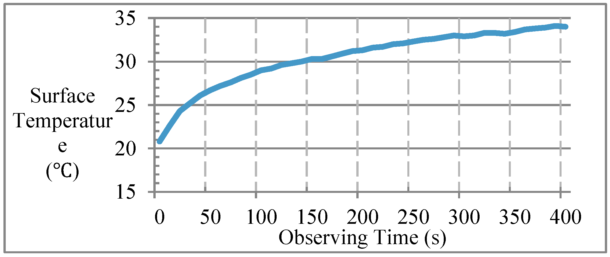
3.3. Laboratory Experiment to Measure the STI

Thermal inertia is an inherent characteristic of soil, and it does not change with the measurements or the meteorological condition. Therefore, in order to assess the accuracy of the simplified thermal inertia values, three categories (three individual samples for each category), including dry clay soil, dry sand soil, and full cover vegetation, are measured in this experiment. In order to prepare the full cover vegetation sample, fresh tree leaves were inserted into a bucket filled with dry sand soil. The VFC value of the full cover vegetation sample is regarded as 1 because of the full cover, and the transpiration is 0. The equipment used in this experiment is shown in the Table 2.

Table 2. Equipment used in the laboratory experiment.

Equipment	Specification of the Accuracy and Unit	Functionality
Net pyranometer	±2%, W/m2	Measuring net radiance
Lamp	Constant radiance at 275 W/m2	Providing downward shortwave and longwave radiation
Infrared thermometer	Model name: Raytek MX4, ±1 °C,automatic recording	Measuring surface temperature

Table 2. Equipment used in the laboratory experiment.

Equipment	Specification of the Accuracy and Unit	Functionality
Net pyranometer	±2%, W/m2	Measuring net radiance
Lamp	Constant radiance at 275 W/m2	Providing downward shortwave and longwave radiation
Infrared thermometer	Model name: Raytek MX4, ±1 °C,automatic recording	Measuring surface temperature

Figure 3. Changes of surface temperature over time for dry clay soil.

Figure 3. Changes of surface temperature over time for dry clay soil.

Table 3. Results of STI.

Samples	Laboratorial Measured Values (J·m−2·K−1·S−1/2)	Estimated Results (J·m−2·K−1·S−1/2)
Dry clay soil	564.6	555.4
Dry sandy soil	560.7
Full covered vegetation	607.2	624.3

Table 3. Results of STI.

Samples	Laboratorial Measured Values (J·m−2·K−1·S−1/2)	Estimated Results (J·m−2·K−1·S−1/2)
Dry clay soil	564.6	555.4
Dry sandy soil	560.7
Full covered vegetation	607.2	624.3

Before the lamp used to simulate the solar radiation was turned on in this experiment, samples had been placed in the laboratory for approximately 24 h in order for the samples to reach the same temperature as that of the laboratory environment. During the experiment (once the lamp was turned on), the net radiation and the surface temperature were automatically recorded at an interval of 10 seconds. For the dry clay soil, the curve of surface temperature change over time is shown in Figure 3. It can be seen from Figure 3 that the rate of temperature rising becomes smaller as time goes by. This is because it takes a few minutes for the sample’s temperature and the surrounding air temperature to approach equilibrium. In order to achieve a better accuracy in the calculations, only the first 10 measurements are used to compute the STI.

The results of STI measurement are shown in Table 3.The standard deviation of STI measurements within each of three categories (sandy, clay, and vegetation) are 8.87, 9.68, and 5.53 J·m⁻²·K⁻¹·S^−1/2, respectively. The average values of three samples in each category are listed in the laboratory measured values of Table 3. It can be seen from Table 3 that STI values from the laboratory measurements are very close to the results estimated in Section 3.2.3. The STI values for dry soil and vegetation both have a bias below 20 J·m⁻²K⁻¹S^−1/2 compared with the estimates from Section 3.2.3. The laboratory experiment verifies that the STI estimates from Section 3.2.3 are reasonable.

4. Regional Application of DDTI and the ET Estimation

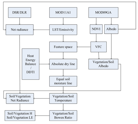
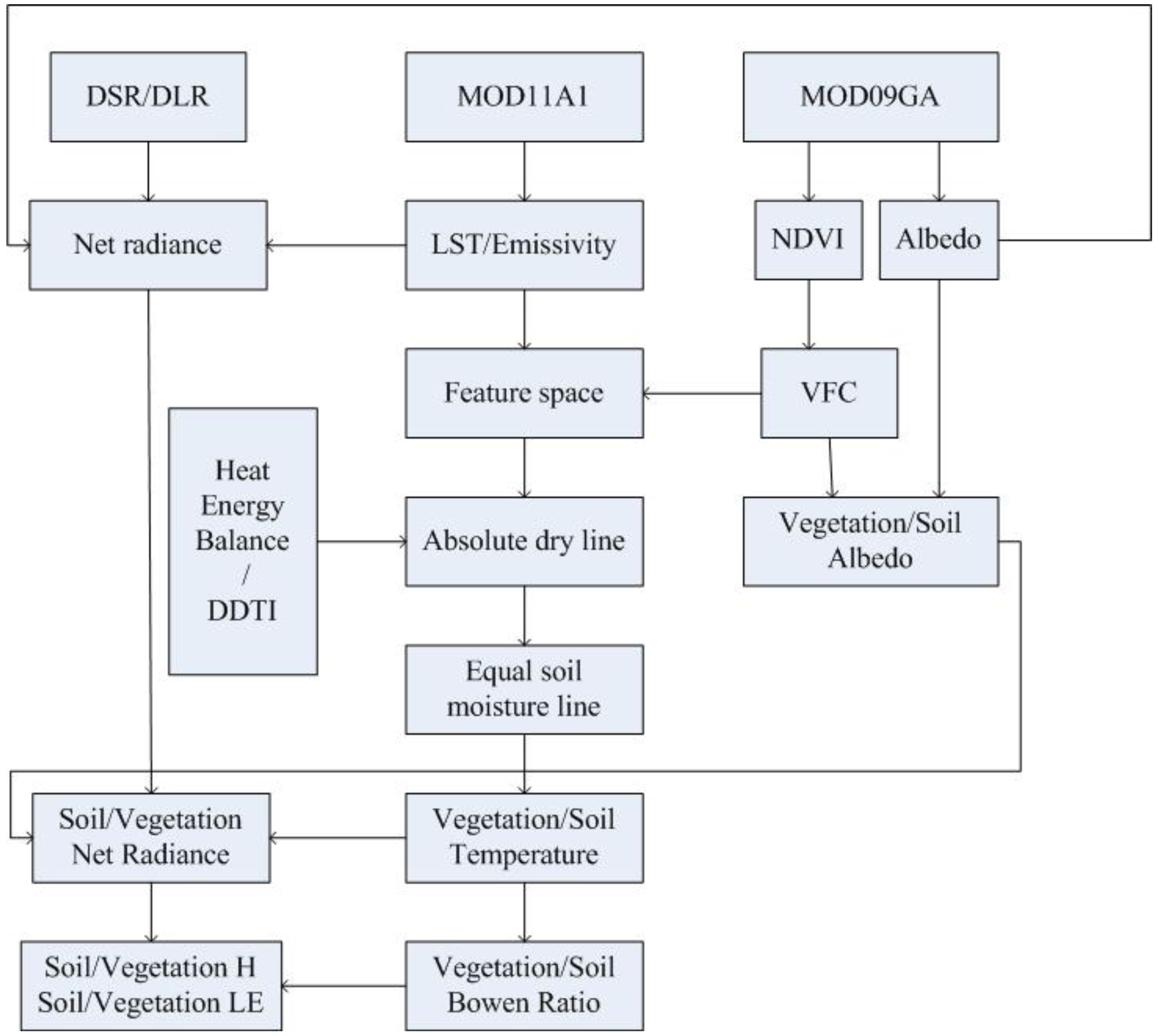
4.1. Computation Processes of the Two Models

Due to the fact that the observation of ET at Yucheng station was not available after year 2011 and the year 2009 showed a high precipitation (101.6 mm) in April and May, days from 1 March 2008 to 30 June 2009, were selected as the study period to estimate the regional ET using DDTI. 21 clear days with cloud cover of less than 10% were chosen based on the MOD11A1 data. There are 13 days selected from year 2008 with four days (3 March, 24 March, 17 April, 29 April) in spring, two days (20 May, 23 August) in summer, six days (1 September, 16 September, 1 October, 19 November, 21 November, and 30 November) in autumn, one day (30 December) in winter. Another eight days are selected from year 2009. One day (1 January) is in winter, five of the days (18 March, 9 April, 21 April, 25 April, and 26 April) are in spring, and 23 May and 5 June are in summer. For the DDTI model, the most suitable simplified thermal inertia values described in Section 3.2.3. were applied to the 21 clear days in order to determine the theoretical dry lines first. The simplified thermal inertia of dry soil P_sd, mean net radiation, start time t_1h, end time t_2h, and start temperature T_1h are fed into Equation (13); then, the theoretical bare soil temperatureT_s2h can be calculated. Similarly, T_v2h can be obtained by Equation (16). After identifying the two endpoints on the theoretical dry line, the theoretical dry line can be determined. For the heat energy balance model, two endpoints were obtained by Equations (5) and (6). In the computations, the daily maximum air temperatures observed separately by eleven weather stations in the study area were used as the air temperatures when determining two endpoints. The aerodynamic resistance is calculated by Equations as follows [25,35]:

$$r=\frac{\ln \left[\frac{z_m-d}{z_{om}}\right]\ln \left[\frac{z_h-d}{z_{oh}}\right]}{k^2{u}_z}$$

(23)

$$z_{oh}=0.1z_{om}$$

(24)

$$d=\left[1-\frac{1-exp\left(-\sqrt{7.5LAI}\right)}{\sqrt{7.5LAI}}\right]\cdot h$$

(25)

$$h=a\frac{LAI}{f}-b$$

(26)

$$z_m=0.1h$$

(27)

where z_m is the height of wind measurements (m), z_h is the height of humidity measurements (m). Generaly, z_h takes the same value with z_m. d is zero plane displacement height (m). z_om is roughness length governing momentum transfer (m). z_oh is the roughness length governing transfer of heat and vapor (m). k is the von Karman’s constant, 0.41. μ_z is the wind speed at height z (m·s⁻¹). h is the crop height. a and b are empirical coefficients and for wheat, they are 0.0093 and 0.0023 m, respectively. For bare land, h and d are zero and z_om is set to 0.04 m [36].

During the period of study, MOD11A1 data, from the land surface temperature product from Moderate-resolution Imaging Spectroradiometer (MODIS) were processed by the MODIS Reprojection Tool (MRT). The albedo data were from MCD43B3 and also processed by the MRT. Other data variables, such as NDVI, and VFC, were processed by the following approaches, with the MOD09GA products being used as the original input.

(1)

NDVI

$$NDVI=\frac{{\text{α}}_1-{\text{α}}_2}{{\text{α}}_1+{\text{α}}_2}$$

(28)

where α₁ and α₂ are the 12th and 11th band in the MOD09GA product.

(2)

VFC

$$VFC=\frac{NDVI-NDV{I}_{min}}{NDV{I}_{max}-NDV{I}_{min}}$$

(29)

where NDVI_max is the maximum value in the NDVI data and NDVI_min is the minimum value in the NDVI data.

(3)

Emissivity

$${\text{ε}}_s=0.273+1.778{\text{ε}}_{31}-1.807{\text{ε}}_{31}{\text{ε}}_{32}-1.037{\text{ε}}_{32}+1.774{\text{ε}}_{32}^2$$

(30)

where ε₃₁ and ε₃₂ are emissivity of the band 31 and the band 32 in MOD11A1 data, ε_s is the land surface emissivity [37].

In this paper, the slope of the theoretical wet line was set to zero. It implies that bare soil or a full cover vegetation area where there is no water stress has the same surface temperature as the theoretical wet line. The temperature of regional bodies of water within the study area was used as the intercept of the theoretical wet line [38].

During the experiment, the Bowen ratio of soil and the Bowen ratio of vegetation can be calculated by the layered energy-separating algorithm of Bowen Ratio. Formulas are provided in Equations (31) and (32) [12,20]. Then, the available energy can be separated into soil evaporation and vegetation transpiration. A detailed introduction can be found in the literature [12,20].

$${\text{β}}_{si}=\frac{T_{sl}-T_{ss}}{T_{sl}-T_{si}}-1$$

(31)

$${\text{β}}_{vi}=\frac{T_{vl}-T_{vs}}{T_{vl}-T_{vi}}-1$$

(32)

where T_sl is the maximum value of separated soil temperature, T_ss is the minimum value of separated soil temperature, T_vl is the maximum value of separated vegetation temperature, T_vs is the minimum value of separated vegetation temperature, T_si is the separated soil temperature of pixel i, and T_vi is the separated vegetation temperature of pixel i.

A flow chart showing the whole process is provided in Figure 4. The equal soil moisture line is a line in which pixels have the same soil moisture and the VFC is the only parameter influencing LST, ignoring influences from other meteorological variables. Equal soil moisture lines are obtained by the ratio of vertical distance to the theoretical dry line and vertical distance to the theoretical wet line. The purpose to determine an equal soil moisture line is to decompose the mixed land surface temperatures in the PCACA model. Two points in one equal soil moisture line, which have same soil temperature and vegetation temperature, can be decomposed by solving linear equations [12,20,25]. The major difference between the two models (DDTI and the heat energy balance model) is how the theoretical dry line is determined.

Figure 4. Flow chart of the ET estimation processes.

Figure 4. Flow chart of the ET estimation processes.

4.2. Results

Three methods were adopted to evaluate the results: the first by comparing the locations of theoretical dry lines, the second by comparing ET results and the third by comparing the evaporative fractions from the two models (DDTI and the heat energy balance model) with the in situ measurements.

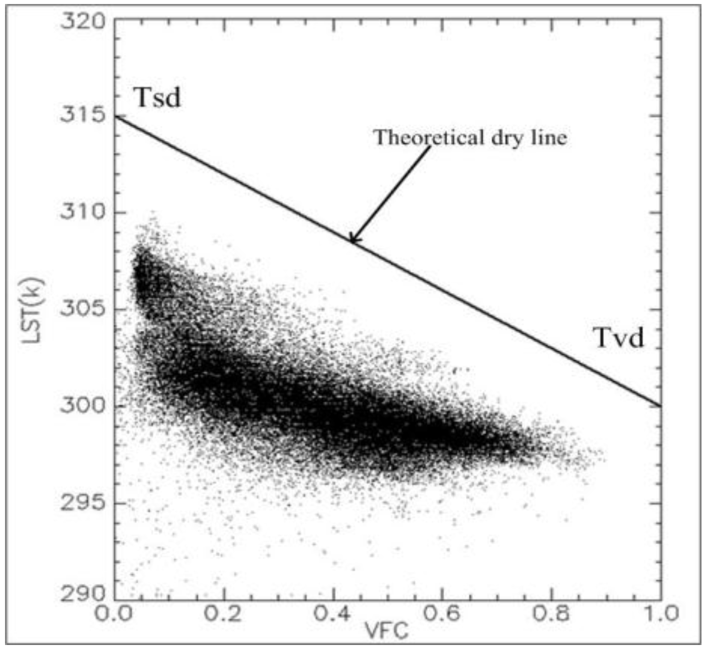
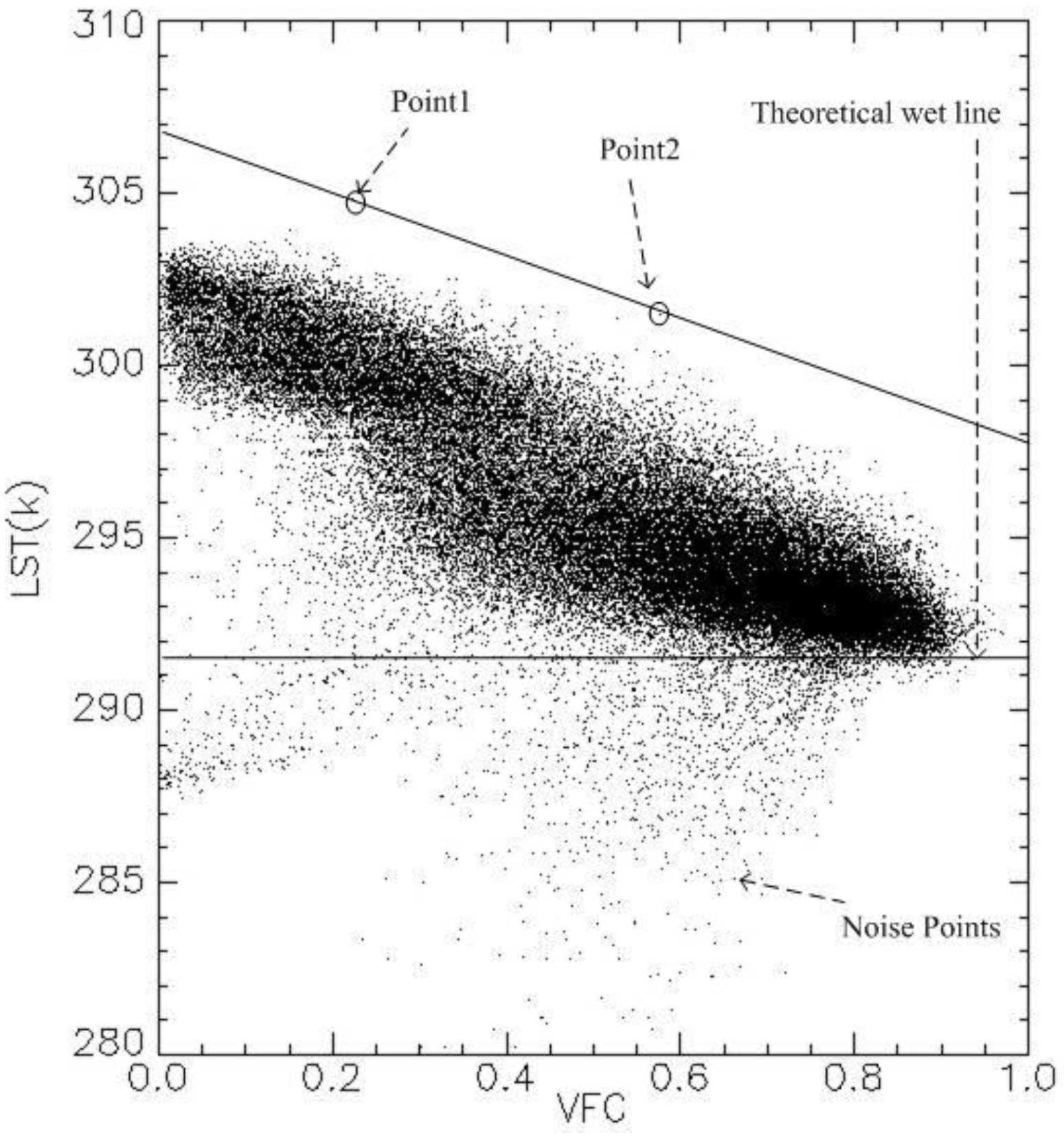
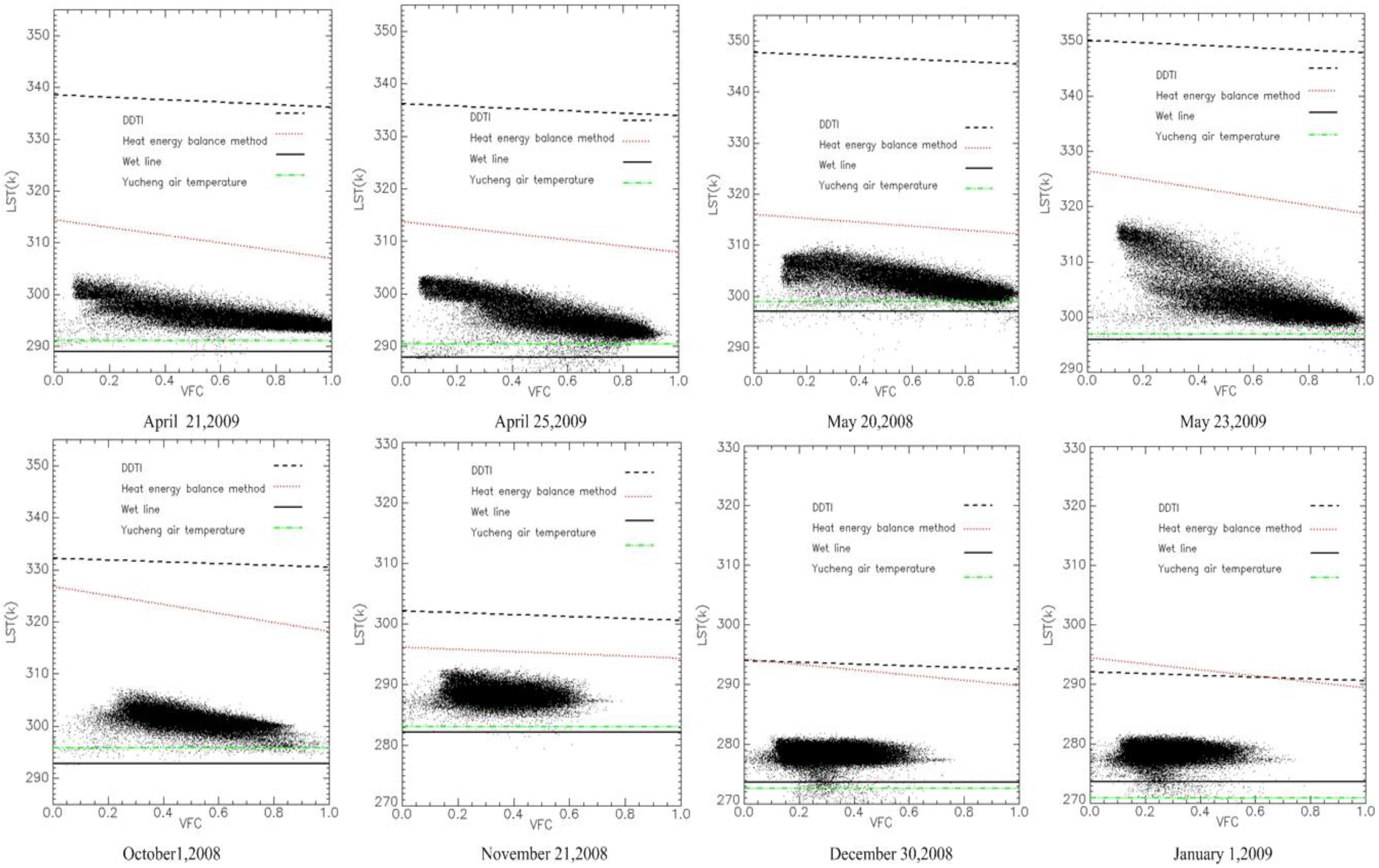
4.2.1. The Location of Theoretical Dry Line

The locations of theoretical dry lines determined from the two models in each season are shown in Figure 5. Two days were selected for each season as representative to compare the two models. Using historical precipitation data from the China Meteorological Sharing Service System, we identified 21 individual dates as representative of either dry periods or wet periods. The cumulative precipitation in the ten days prior to 3 March, 19 November, 21 November, 30 November, 30 December, 1 January, 18 March, and 9 April was less than 3 mm and these eight days are considered to be dry periods. The other 13 days are considered to be humid or sub-humid periods. Some meteorological variables at the overpassing time of 21 MODIS scenes are shown in Table 4. It can be seen from Figure 5 that the locations of theoretical dry lines determined by the heat energy balance model are closer to the scatter cloud and lower than theoretical dry lines determined by DDTI model except the Winter, indicating that the line from DDTI shows a dryer condition than that from the heat energy balance model in the spring, summer and autumn. In the winter, lines of two days are almost the same, which indicating that the two models have the same effect to determine dry lines in dry period. It can also be seen from Figure 5 that, in wet days, such as 23 May 2008 and 25 May 2009, values of T_sd by the DDTI model are 30 K higher than the highest land surface temperature of the area, while values of T_sd from the heat energy balance model are only about 10 K higher than the highest land surface temperature of the area. T_sd of about 10 K higher than land surface temperature turns out to be unreasonable for wet areas. So, the DDTI model is more reasonable than heat energy balance model in wet areas. The intercept of the theoretical dry line can be as high as 350 K, which can be explained by the definition of the theoretical dry line, since it refers to the historical extreme dry situation. The DDTI model presented in this paper can be used not only in two-layer ET models, but also can be used in one-layer feature space schemes. The air temperatures observed at the satellite overpass time in Yucheng and the wet lines for eight dates are also shown in Figure 5. It can be seen from Figure 5 that, air temperatures in Yucheng are usually higher than the wet lines except on 30 December 2008 and 1 January 2009. The temperature of the water body, which was measured at the center of a lake from the MODIS LST data product to determine the wet line, is more stable than the air temperature in Yucheng at the satellite overpass time. During late December and early January when is in cold winter, the air temperature in Yucheng at the satellite overpass time can be 2 or 3 degrees lower than the temperature of the water body which was close to zero degrees Celsius. It appears that using the temperature of water body as wet lines is more reasonable.

Table 4. Meteorological variables at the MODIS overpassing time at Yucheng Station.

Variables Date	Overpass Time in Local	S0 (W/m2)	Ta (°C)	Wind Speed (m/s)	Air Relative Humidity (%)
3 March 2008	11 a.m.	700.5	7.9	4.457	24.9
24 March 2008	11:18 a.m.	806	10.85	0	24.18
17 April 2008	10:30 a.m.	730.7	20.37	4.22	66
29 April 2008	10:54 a.m.	718.1	23.29	1.8	47.11
20 May 2008	10:54 a.m.	831	25.8	6.7	50
23 August 2008	10:30 a.m.	722.1	28.42	2.098	68.04
1 September 2008	10:24 a.m.	749.9	25	1.22	51.5
6 September 2008	10:30 a.m.	606.5	27.3	1.277	58.04
1 October 2008	10:30 a.m.	661.2	22.71	2.77	57
19 November 2008	11:18 a.m.	533.3	4.8	0.921	27.1
21 November 2008	11:6 a.m.	469.4	9.94	3.69	34.52
30 November 2008	11 a.m.	445.1	10.73	4.1	33.78
30 December 2008	11:12 a.m.	469.4	−0.5	3.69	27.85
1 January 2009	11 a.m.	441	−2.25	0	34.9
18 March 2009	11:24 a.m.	659.9	21.93	4.48	52.5
9 April 2009	10:48 a.m.	782.2	20.87	3.3	41.4
21 April 2009	11:12 a.m.	873	17.9	2.6	37.2
25 April 2009	10:48 a.m.	831	17.3	2.9	35.5
26 April 2009	11:30 a.m.	854	18	2.1	30
23 May 2009	10:40 a.m.	937	23.73	2.5	50.6
5 June 2009	10:42 a.m.	754	30.12	2.35	41.75

Table 4. Meteorological variables at the MODIS overpassing time at Yucheng Station.

Variables Date	Overpass Time in Local	S0 (W/m2)	Ta (°C)	Wind Speed (m/s)	Air Relative Humidity (%)
3 March 2008	11 a.m.	700.5	7.9	4.457	24.9
24 March 2008	11:18 a.m.	806	10.85	0	24.18
17 April 2008	10:30 a.m.	730.7	20.37	4.22	66
29 April 2008	10:54 a.m.	718.1	23.29	1.8	47.11
20 May 2008	10:54 a.m.	831	25.8	6.7	50
23 August 2008	10:30 a.m.	722.1	28.42	2.098	68.04
1 September 2008	10:24 a.m.	749.9	25	1.22	51.5
6 September 2008	10:30 a.m.	606.5	27.3	1.277	58.04
1 October 2008	10:30 a.m.	661.2	22.71	2.77	57
19 November 2008	11:18 a.m.	533.3	4.8	0.921	27.1
21 November 2008	11:6 a.m.	469.4	9.94	3.69	34.52
30 November 2008	11 a.m.	445.1	10.73	4.1	33.78
30 December 2008	11:12 a.m.	469.4	−0.5	3.69	27.85
1 January 2009	11 a.m.	441	−2.25	0	34.9
18 March 2009	11:24 a.m.	659.9	21.93	4.48	52.5
9 April 2009	10:48 a.m.	782.2	20.87	3.3	41.4
21 April 2009	11:12 a.m.	873	17.9	2.6	37.2
25 April 2009	10:48 a.m.	831	17.3	2.9	35.5
26 April 2009	11:30 a.m.	854	18	2.1	30
23 May 2009	10:40 a.m.	937	23.73	2.5	50.6
5 June 2009	10:42 a.m.	754	30.12	2.35	41.75

Figure 5. Locations of the theoretical wet/dry lines from two models in each season.

Figure 5. Locations of the theoretical wet/dry lines from two models in each season.

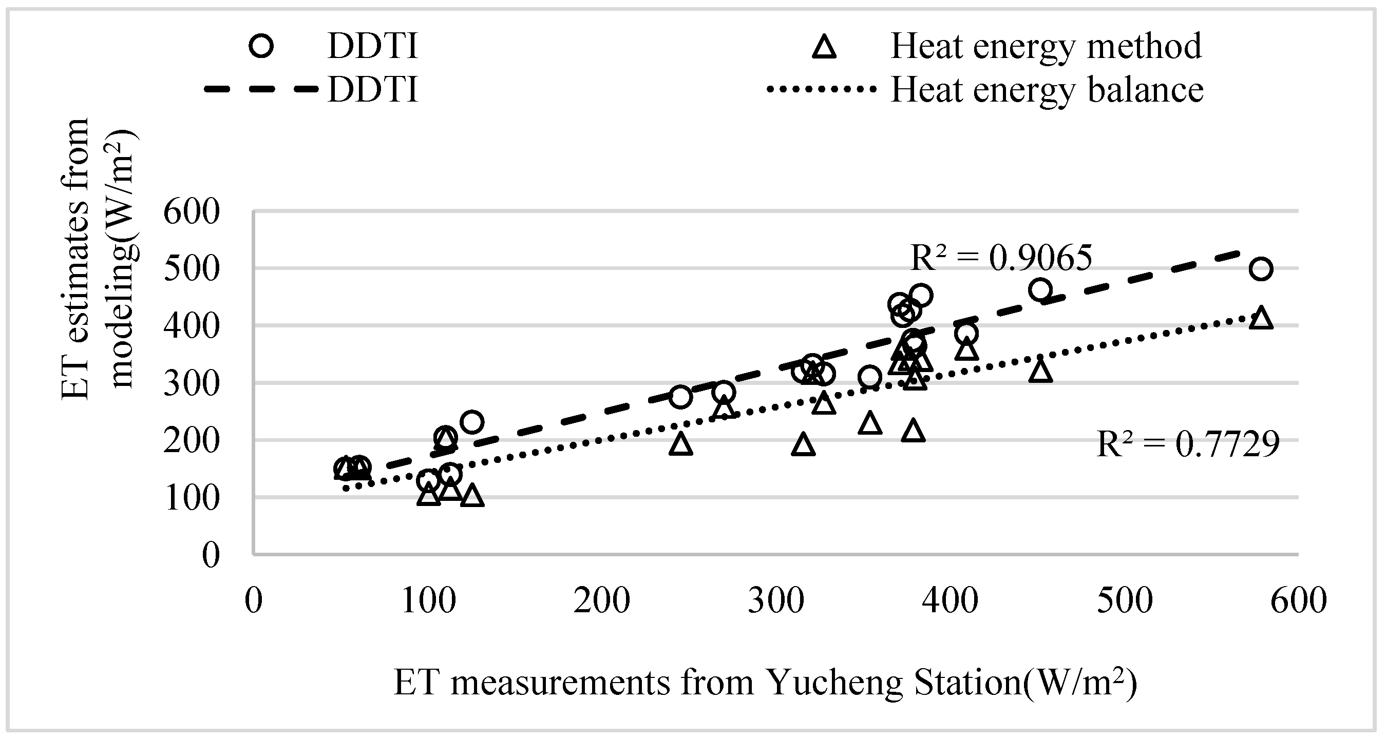
4.2.2. Comparison of ET Results

Estimates of ET results from the two models were compared with the in situ messurements at the Yucheng Station. Comparison result are shown in Figure 6. LE appeared to be well estimated by the two models. DDTI demonstrated ET with a root mean square error (RMSE) of 56.77 W/m² and a bias of 27.17 W/m²; while the heat energy balance model demonstrated an RMSE of 83.36 W/m² and a bias of −38.42 W/m². For comparing the coeffcient of determination for the two models, DDTI demonstrated ET with R² of 0.9065; while the heat energy balance model has that of 0.7729. The DDTI results were statistically closer to the observations.

Figure 6. ET estimates from two models.

Figure 6. ET estimates from two models.

The evapotranspiration results on 18 March and 21 April of 2009 by the DDTI model are shown in Figure 7. These two days are representative of dry days and wet days, separately. It can be seen from Figure 7 that the evapotranspiration on 21 April is larger than that of 18 March in 2009, because 21 April was wetter than 18 March. In both images, the areas with the largest evapotranspiration are bodies of water. Since the northwest region of the study area was mainly composed of cotton growing area, it was bare land in March and April, so evapotranspiration is much less than other areas, which are winter wheat fields or mountain forest. Areas with no evapotranspiration values (shown in white) are cloud-contaminated pixels.

Figure 7. Regional ET of 18 March and 21 April.

Figure 7. Regional ET of 18 March and 21 April.

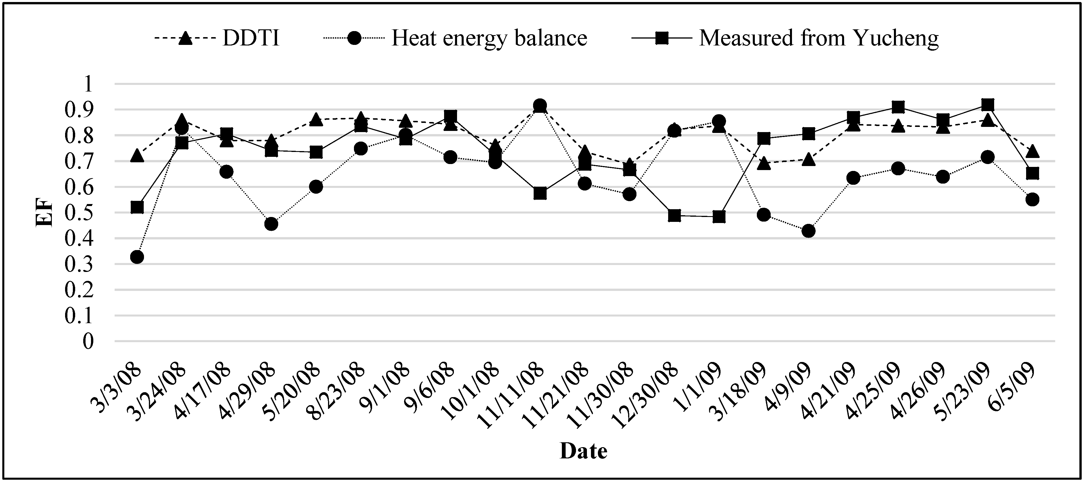
4.2.3. Comparison of Evaporative Fraction from the Two Models

In order to further analyze the performance of the theoretical dry line determination by DDTI, the Evaporative Fraction (EF) was selected as a criterion to evaluate the two models. EF is defined as the ratio of ET to the available energy [39].

$$EF=\frac{LE}{R_n-G}$$

(33)

Figure 8. Comparison of EF of the two models.

Figure 8. Comparison of EF of the two models.

EF values observed by Yucheng station, estimated by the heat energy balance model and by DDTI in the 21 clear days, are shown in Figure 8. When compared with the in situ measurements of EF at Yucheng Experimental Station, the ET model based on DDTI reproduces the pixel scale EF with an RMSE of 0.151, which is much lower than that based on the heat energy balance model (an RMSE of 0.220). Also, the bias between DDTI and in situ measurements is 0.064 lower than the bias of the heat energy balance model, which is −0.084. It shows that the DDTI model provided more accurate estimates than the heat energy balance model.

5. Discussions

5.1. Comparison with Other Studies

Extensive validation and inter-comparison studies of remote sensing-based evapotranspiration models had been conducted using dataset from the Yucheng station [40,41,42,43,44]. Sun [41] presented a study to retrieve ET based on MODIS data and Yucheng Station was selected to validate the model. The study from Sun showed that the Sim-ReSET model had instantaneous ET estimation with a mean absolute difference (MAD) of 34.27 W/m² and a root mean square error (RMSE) of 41.84 W/m² [40,41]. Liu presented ET retrievals from MODIS data during year 2005–2006 over the Yucheng station, which had the consistency index of 0.917, correlation coefficient of 0.872 with the measurements by a lysimeter [42]. Tang compared three remote sensing-based energy balance models using lysimeter during the wheat (late April to late May) and corn (early July to late September) growing periods excluding the maturity stage of year 2009. The three models were the surface energy balance system (SEBS), the two-source energy balance (TSEB) model and the surface temperature-vegetation index triangle (TVT). When estimating ET with the same dataset, the TSEB model showed an agreement with the Lysimeter observed result with an RMSE of about 45 W/m², while the SEBS showed an RMSE of about 55 W/m² and TVT showed an RMSE higher than 110 W/m² [43]. Tian presented ET estimates with an operational two-layer model in North China based on MODIS data in year 2004 from March to June, which showed that the correlation coefficient between the estimated surface ET and the observations from Yucheng station was 0.85 and the RMSE is 21.3 W/m² [44].

The ET estimates from the DDTI model have an RMSE of 56.77 W/m², a bias of 27.17 W/m², and an R² of 0.9065, while the EF by the DDTI model have an RMSE of 0.149, a bias of 0.064. The accuracy of the ET results by DDTI is comparable to the prior studies. The DDTI result have a smaller bias than Sim-ReSET and a higher R² than Sim-ReSET and Tian’s result, which indicates that the theoretical dry line determined by the DDTI is more reasonable. Sim-ReSET and TSEB both show a lower RMSE than DDTI because all four different seasons are included in the DDTI estimates, however, the other models focused only on the crop growing seasons.

5.2. Advantages of DDTI

The most significant contribution of DDTI is its capability to determine the theoretical dry line in wet period without the need of aerodynamic resistance and air temperature at the satellite overpassing time. This feature would be more beneficial in ET estimation compared with the heat energy balance model and other feature space models. In particular, DDTI is featured with the following advantages:

(1)

DDTI is especially advantageous for applications in area of wet situation where no dry pixels exist. In the feature space models, it is more difficult to determine the dry line than the wet line since dry pixels do not exist in many situations. The determination of the dry line is somewhat subjective and, thus, inaccurate. Therefore, the locations of dry line are usually underestimated. The DDTI model estimates the theoretical dry line by the soil characteristics, which are determined from historical extremely dry situations, without the need of land surface temperature at the satellite overpassing time.

(2)

DDTI does not need the parameterization of the aerodynamic resistance which is required in other ET models, such as the heat energy balance model. Consequently, some other parameters which are needed to estimate aerodynamic resistance (e.g., canopy height, roughness) are not required. The aerodynamic resistance is usually difficult to available at regional scales. Not using the aerodynamic resistance is another advantage of DDTI.

(3)

DDTI requires relatively fewer inputs. Meteorological variables such as air temperature, air humidity, and wind speed at satellite overpass time are not needed in this model. It has to be noted that air temperature and air humidity are required variables for many ET models, such as the heat energy balance model.

(4)

The DDTI model can be integrated not only in two-layer ET models, but also can be used in one-layer feature space schemes.

5.3. Limitations of DDTI

(1)

A special category of observations from ground is needed in DDTI. Some parameters, such as land surface temperature and local time when net radiance is equal to 0, are needed. The application of this method is limited in areas which don’t have this data.

(2)

DDTI needs the STI values of bare land and vegetation fully covered area. In this paper, they are determined by a historical dataset. A laboratory experiment was also used to measure the STI. DDTI cannot be used in areas without a historical extremely dry period.

(3)

Soil texture is not considered in DDTI. Soil texture is assumed to be uniform when estimating STI from remote sensing images in this paper. When DDTI is used in area with heterogeneous soil texture, it is more reasonable to adjust the STI values to account for the soil texture, which will be studies in the future.

(4)

DDTI was evaluated in North China Plain in this present study. Performance of DDTI is to be evaluated in the regions with different climatology. MODIS images used in this paper have a resolution of 1km. Satellite sensors with a finer spatial resolution, such as Landsat TM and HJ 1B, will be used in the future study.

6. Conclusions

In this study, we developed a new model named DDTI to determine the theoretical dry line. The Simplified Thermal Inertia was first estimated by satellite observations in the North China Plain, and then validated by a laboratory experiment. DDTI was applied to the 13 clear days from 2008 and eight clear days from 2009 in the North China Plain to estimate the regional ET. Finally, the EF observed by an experimental station was used to assess the accuracy of ET retrieval. Several conclusions can be made from this study:

(a)

The STI values estimated in the North China Plain in dry situations are consistent with the measurements in the laboratory experiment, which is a solid basis for the DDTI model.

(b)

The theoretical dry line determined by the DDTI is all above the scatter cloud in the feature space and also higher than that by the heat energy balance model in spring, summer, and autumn. The theoretical dry lines determined by the two models are almost the same in winter. The theoretical dry line determined by the DDTI appears more reasonable and robust than the line determined by the heat energy balance model, especially in wet period.

(c)

Validation of DDTI was done by comparing the ET estimates from 21 scenes of MODIS images and the Eddy covariance measurements at Yucheng Station. ET estimated from DDTI has an root mean square error (RMSE) of 56.77 W/m² and a bias of 27.17 W/m²; while the heat energy balance model estimated ET with an RMSE of 83.36 W/m² and a bias of −38.42 W/m². When comparing the coeffcient of determination of two models with data from Yucheng, DDTI demonstrated ET with R² of 0.9065; while the heat energy balance model has that of 0.7729. When compared with the in situ measurement of evaporative fraction (EF) at Yucheng Experimental Station, the ET model based on DDTI reproduces the pixel scale EF with an RMSE of 0.149, much lower than that based on the heat energy balance model which has an RMSE of 0.220. Also, the EF bias between the DDTI model and the in situ measurements is 0.064, lower than the EF bias of the heat energy balance model, which is −0.084.This reveals that the DDTI model gives better estimates of ET than the heat energy balance model, and it can be applied to both wet conditions and dry conditions.

References

1. Choudhury, B.J. Estimating evaporation and carbon assimilation using infrared temperature data: Vistas in modeling. In Theory and Applications of Remote Sensing; Asrar, G., Ed.; John Wiley: New York, NY, USA, 1989; pp. 628–690. [Google Scholar]
2. Kustas, W.P.; Norman, J.M. Use of remote sensing for evapotranspiration monitoring over land surfaces. Hydrol. Sci. J. 1996, 41, 495–517. [Google Scholar] [CrossRef]
3. Moran, C.A.; Jackson, R.D. Assessing the spatial distribution of evapotranspiration using remotely sensed inputs. J. Environ. 1991, 20, 725–737. [Google Scholar] [CrossRef]
4. Jiang, L.; Islam, S. A methodology for estimation of surface evapotranspiration over large areas using remote sensing observations. Geophys. Res. Lett. 1999, 26, 2773–2776. [Google Scholar] [CrossRef]
5. Jiang, L.; Islam, S. Estimation of surface evaporation map over southern Great Plains using remote sensing data. Water Res. 2001, 37, 329–340. [Google Scholar] [CrossRef]
6. Allen, R.G.; Tasymi, M.; Trezza, R. Satellite-based energy balance for mapping evapotranspiration with internalized calibration (METRIC)-model. J. Irrig. Drain. Eng. 2007, 133, 380–394. [Google Scholar] [CrossRef]
7. Bastiaanssen, W.G.M.; Menenti, M.; Feddes, R.A.; Holslag, A.A.M. A remote sensing surface energy balance algorithm for land (SEBAL). 1. Formulation. J. Hydrol. 1998, 212, 198–212. [Google Scholar] [CrossRef]
8. Su, Z.B. The Surface Energy Balance System (SEBS) for estimation of turbulent heat fluxes. Hydrol. Earth Sys. Sci. 2002, 6, 85–99. [Google Scholar] [CrossRef]
9. Roerink, G.J.; Su, Z.B.; Menenti, M. S-SEBI: A simple remote sensing algorithm to estimate the surface energy balance. Phys. Chem. Earth (B) 2000, 25, 147–157. [Google Scholar] [CrossRef]
10. Norman, J.M.; Kustas, W.P.; Humes, K.S. Source approach for estimating soil and vegetation energy fluxes in observations of directional radiometric surface temperature. Agr. For. Meteor. 1995, 77, 263–293. [Google Scholar] [CrossRef]
11. Kustas, W.P.; Norman, J.M. A two-source energy balance approach using directional radiometric temperature observations for space canopy covered surfaces. Agr. J. 2000, 92, 847–854. [Google Scholar] [CrossRef]
12. Zhang, R.H.; Sun, X.M.; Wang, W.M.; Xu, J.P.; Zhu, Z.L.; Tian, J. An operational two-layer remote sensing model to estimate surface flux in regional scale: Physical background. Sci. China Ser. D Earth Sci. 2005, 48, 225–244. [Google Scholar]
13. Kustas, W.P.; Norman, J.M. Evaluation of soil and vegetation heat flux predictions using a simple two source model with radiometric temperatures for partial canopy cover. Agr. For. Meteor. 1999, 94, 13–29. [Google Scholar] [CrossRef]
14. Xu, Z.X.; Li, J.Y. Estimating basin evapotranspiration using distributed hydrologic model. J. Hydrol. Eng. 2003, 2, 74–80. [Google Scholar] [CrossRef]
15. Price, J.C. Using spatial context in satellite data to infer regional scale evapotranspiration. IEEE Trans. Geophys. Remote Sens. 1990, 28, 940–949. [Google Scholar] [CrossRef]
16. Moran, M.S.; Clarke, T.R.; Inoue, Y.; Vidal, A. Estimation crop water deficit using the relation between surface-air temperature and spectral vegetation index. Remote Sens. Environ. 1994, 49, 246–263. [Google Scholar] [CrossRef]
17. Nishida, K.; Nemani, R.R.; Running, S.W.; Glassy, J.M. An operational remote sensing algorithm of land surface evaporation. J. Geo. Res. 2003, 108, 4270. [Google Scholar] [CrossRef]
18. Merlin, O. An original interpretation of the wet edge of the surface temperature-albedo space to estimate crop evapotranspiration (SEB-1S), and its validation over an irrigated area in northwestern Mexico. Hydrol. Earth Sys. Sci. 2013, 17, 3623–3637. [Google Scholar] [CrossRef] [Green Version]
19. Meilin, O.; Chirouze, J.; Olioso, A.; Jarlan, L.; Chehbouni, G.; Boulet, G. An image-based four source surface energy balance model to estimate crop evapotranspiration from solar reflectance/thermal emission data (SEB-4S). Agr. For. Meteor. 2014, 184, 188–203. [Google Scholar]
20. Zhang, R.H.; Tian, J.; Sun, X.M.; Chen, S.H.; Xia, J. Two improvements of an operational two-layer model for terrestrial heat flux retrieval. Sensors 2008, 8, 6165–6187. [Google Scholar] [CrossRef]
21. Tang, R.L.; Li, Z.L.; Tang, B.H. An application of the TS-VI triangle method with enhanced edges determination for evapotranspiration estimation from MODIS data in arid and semi-arid regions: Implementation and Validation. Remote Sens. Environ. 2010, 114, 540–551. [Google Scholar] [CrossRef]
22. Bastiaanssen, W.G.M. SEBAL-based sensible and latent heat fluxes in the irrigated Gediz Basin, Turkey. J. Hydrol. 2000, 229, 87–100. [Google Scholar] [CrossRef]
23. Long, D.; Singh, V.P. A two-source trapezoid model for evapotranspiration (TTME) from satellite imagery. Remote Sens. Environ. 2012, 121, 370–388. [Google Scholar] [CrossRef]
24. Price, J.C. On the analysis of thermal infrared imagery: The limited utility of apparent thermal inertia. Remote Sens. Environ. 1985, 18, 59–73. [Google Scholar] [CrossRef]
25. Zhang, R.H. Quantitative Model of Thermal Infrared Remote Sensing and Ground Experiments. Beijing; Science Press: Beijing, China, 2009; pp. 274–279. [Google Scholar]
26. Robin, L.F.; Philip, R.C.; Hugh, H.K. High-resolution thermal inertia derived from the thermal emission imaging system (THEMIS): Thermal model and applications. J. Geophys. Res. 2006, 111, 1–22. [Google Scholar]
27. Price, J.C. Thermal inertia mapping: A new view of the earth. J. Geophys. Res. 1977, 82, 2582–2590. [Google Scholar] [CrossRef]
28. Pratt, D.A.; Ellyett, C.D. The thermal inertia approach to mapping of soil moisture and geology. Remote Sens. Environ. 1979, 8, 151–168. [Google Scholar] [CrossRef]
29. Sobrino, J.A.; EI Kharraz, M.H. Combining afternoon and morning NOAA satellites for thermal inertia estimation: Methodology and application. J. Geophys. Res. 1999, 104, 9455–9465. [Google Scholar] [CrossRef]
30. Kahle, A.B.; Gillespie, A.R.; Goetz, F.H. Thermal inertia imaging: A new geologic mapping tool. Geophys. Res. Lett. 1976, 3, 23–28. [Google Scholar] [CrossRef]
31. Tramutoli, V.; Claps, P.; Marella, M.; Pergola, N.; Sileo, C. Feasibility of hydrological application of thermal inertia from remote sensing. In Proceedings of the 2nd Plinius Conference on Mediterranean Storms, Siena, Italy, 16–18 October 2000; pp. 16–18.
32. Cracknell, A.P.; Xue, Y. Thermal inertia determination from space—A tutorial review. Int. J. Remote Sens. 1996, 17, 431–461. [Google Scholar] [CrossRef]
33. Zhang, R.H. Investigation of remote sensing of soil moisture. In Proceedings of the Fourteenth International Symposium on Remote Sensing of Environment V.I., San Jose, Costa Rica, 23–30 April 1980; pp. 121–133.
34. Short, N.; Stuart, L., Jr. The Heat Capacity Mapping Mission (HCMM) Anthology; Scientific and Technical Information Branch, National Aeronautics & Space Administration: Washington, DC, USA, 1983. [Google Scholar]
35. Fao corporate document repository. Available online: http://www.fao.org/docrep/x0490e/x0490e06.htm#aerodynamicresistance (ra) (assessed on 18 August 2015).
36. Jia, L.; Wang, J.M.; Massimo, M. Estimation of area roughness length for momentum using remote sensing data and measurements in field. Chin. J. Atmos. Sci. 1999, 23, 632–643. [Google Scholar]
37. Liang, S.L. Quantitative Remote Sensing of Land Surface; John Wiley & Sons: Hoboken, NJ, USA, 2004. [Google Scholar]
38. Carlson, T. Evapotranspiration and soil moisture from satellite imagery. Sensors 2007, 7, 1612–1629. [Google Scholar] [CrossRef]
39. Shuttleworth, W.J.; Gurney, R.J.; Hsu, A.Y.; Ormsby, J.P. FIFE: The variation in energy partition at surface flux sites. In Remote Sensing and Large-Scale Processes, Proceedings of the IAHS Third International Assembly, Baltimore, MD, USA, 10–19 May 1989; IAHS Publication: Baltimore, MD, USA, 1989; Volume 186, pp. 67–74. [Google Scholar]
40. Sun, Z.G.; Wang, Q.X.; Matsushita, B.; Fukushima, T.; Ouyang, Z.; Watanabe, M. Development of a simple remote sensing evapotranspiration model (Sim-ReSET): Algorithm and model test. J. Hydrol. 2009, 376, 476–485. [Google Scholar] [CrossRef] [Green Version]
41. Sun, Z.; Wang, Q.; Matsushita, B.; Fukushima, T.; Ouyang, Z.; Gebremichael, M. A simple model for estimating evapotranspiration based solely on remote sensing: Algorithm and application. In AGU Fall Meeting Abstracts, Proceedings of the AGU Fall Meeting, San Francisco, CA, USA, 14–18 December 2009; Volume 1, p. 769.
42. Liu, C.; Gao, W.; Gao, Z.; Shi, R. Application of MODIS data for assessment of evapotranspiration and drought in Northern China. In SPIE Proceedings, Proceedings of the Remote Sensing and Modeling of Ecosystems for Sustainability VI, San Diego, CA, USA, 2 August 2009; Gao, W., Jackson, J.G., Eds.; International Society for Optics and Photonics: Belek-Antalya, Tuekey, 2009; p. 74541. [Google Scholar]
43. Tang, R.; Li, Z.L.; Jia, Y.; Li, C.R.; Sun, X.M.; Kustas, W.P.; Anderson, M.C. An intercomparison of three remote sensing-based energy balance models using large aperture scintillometer measurements over a wheat-corn production region. Remote Sens. Environ. 2011, 115, 3187–3202. [Google Scholar] [CrossRef]
44. Tian, J.; Su, H.; Sun, X.; Chen, S.H. Application of an operational two-layer model for soil evaporation and vegetation transpiration retrievals in North China. Geogr. Res. 2009, 28, 1297–1306. [Google Scholar]