Article

World’s Largest Macroalgal Blooms Altered Phytoplankton Biomass in Summer in the Yellow Sea: Satellite Observations

1
Key Laboratory of Coastal Environmental Processes and Ecological Remediation, Yantai Institute of Coastal Zone Research, Chinese Academy of Sciences, 17 Chunhui Road, Laishan District, Yantai 264003, China
2
The Sino-Australian Research Centre for Coastal Management, School of Physical, Environmental and Mathematical Sciences, University of New South Wales at the Australian Defence Force Academy, Northcott Drive, Canberra, ACT 2600, Australia
3
College of Marine Science, University of South Florida, 140 Seventh Avenue, South, St. Petersburg, FL 33701, USA
4
State Key Laboratory of Tropical Oceanography, South China Sea Institute of Oceanology, Chinese Academy of Sciences, 164 Xingang West Road, Guangzhou 510301, China
5
State Key Laboratory of Information Engineering in Surveying, Mapping and Remote Sensing, Wuhan University, 129 Luoyu Road, Wuhan 430079, China
*
Author to whom correspondence should be addressed.
Remote Sens. 2015, 7(9), 12297-12313; https://0-doi-org.brum.beds.ac.uk/10.3390/rs70912297
Submission received: 28 April 2015 / Revised: 29 July 2015 / Accepted: 11 September 2015 / Published: 21 September 2015
(This article belongs to the Special Issue Remote Sensing of Biogeochemical Cycles)

Abstract

:
Since 2008, the world’s largest blooms of the green macroalgae, Ulva prolifera, have occurred every summer in the Yellow Sea, posing the question of whether these macroalgal blooms (MABs) have changed the phytoplankton biomass due to their perturbations of nutrient dynamics. We have attempted to address this question using long-term Moderate Resolution Imaging Spectroradiometer (MODIS) observations. A new MODIS monthly time-series of chlorophyll-a concentrations (Chl-a, an index of phytoplankton biomass) was generated after removing the macroalgae-contaminated pixels that were characterized by unexpectedly high values in the daily Chl-a products. Compared with Chl-a during July of 2002–2006 (the pre-MAB period), Chl-a during July of 2008–2012 (the MAB period) exhibited significant increases in the offshore Yellow Sea waters (rich in macroalgae), with mean Chl-a increased by 98% from 0.64 µg/L to 1.26 µg/L in the study region. In contrast, no significant Chl-a changes were observed during June between the two periods. After analyzing sea surface temperature, photosynthetically available radiation, and nutrient availability, we speculate that the observed Chl-a changes are due to nutrient competition between macroalgae and phytoplankton: during the MAB period, the fast-growing macroalgae would uptake the increased nutrients from the origin of Jiangsu Shoal; thus, the nutrients available to phytoplankton were reduced, leading to no apparent increases in biomass in the offshore Yellow Sea in June.

Graphical Abstract

1. Introduction

Macroalgal blooms (MABs), caused by the fast growth and accumulation of macroalgae, have increased remarkably in the global oceans in recent years [1], and thus it is pressing to understand the ecological consequences of these blooms [2]. Since 2008, the world’s largest MABs of Ulva prolifera (also called green tides) have occurred every summer in the Yellow Sea [3,4,5,6] (Figure 1). These MABs have occurred in the semi-enclosed ocean basins, which have resulted in significant impacts on local marine ecosystems and local economy [7]. Several studies have documented the occurrence statistics and causes of these MABs through satellite remote sensing, in situ measurements, and laboratory analysis, with the following findings: (a) the Jiangsu Shoal served as the seed source of the MABs [4,5,8,9], where the pathway of floating macroalgae was numerically modeled and validated by satellite observations [4,10]; (b) the area influenced by MABs ranged from the East China Sea to the Yellow Sea, extending to the west coast of South Korea, as shown in Xing et al. [9]; (c) in late April and early May, driven by the Jiangsu coastal current and the North-East Asia Monsoon (NEAM), macroalgae drifted to the East China Sea; then, with the strengthening of summer NEAM, macroalgae moved northward to enter the southern Yellow Sea and reached the southern coast of Shandong Peninsula in June and July [9]; and (d) as shown by the satellite images of maximum daily MAB area, the most severely influenced area was the offshore region near Qingdao, where the impacted area varied in different years, with the maximum bloom area found in 2008 [6].
The growth of macroalgae might reduce phytoplankton biomass through nutrient competition [11,12]: macroalgae in the growing and expanding stage consumed nutrients in water column and reduced nutrient availability to phytoplankton. In addition, the release of nutrients due to decomposition of macroalgae might also stimulate the growth of phytoplankton [13]. For the world’s largest MABs in the Yellow Sea [5,8], it is difficult to assess the interactions between macroalgae and phytoplankton in such a large region through in situ observations [11,12,13]; to date, there has been no such report for the Yellow Sea, possibly due to difficulties in assessing long-term alternations in phytoplankton in the presence of macroalgae.
Thus, the objective of this study is to document potential phytoplankton biomass changes associated with the MABs in the Yellow Sea through synoptic satellite ocean color observations. Indeed, such observations have been used to document the transport of phytoplankton blooms in the Bohai Sea [14] and the South China Sea [15] as well as to study global- to basin-scale phytoplankton changes. In this work, chlorophyll-a concentration (Chl-a) from the satellite measurement was regarded as an index of phytoplankton biomass, and the Chl-a time-series were used to evaluate the impacts of MABs on the water-column phytoplankton in the Yellow Sea.
Figure 1. Study region showing the area impacted by MABs (green slicks in and near the purple dashed circle) during summer 2008 in the Yellow Sea. The arrow shows the main drifting pathway of macroalgae from the origin of Jiangsu Shoal, the most nutrient-polluted region in the Yellow Sea. The green slicks of macroalgae were extracted from Moderate Resolution Imaging Spectroradiometer (MODIS) measurements on day 136, 151, 170, and 180 in 2008 using the data of MODIS Normalized Difference Vegetation Index (NDVI) [6]. The green dots show the macroalgae origin sites validated from a cruise survey in 2009. Box A is a pilot region (35.5°N –36°N, 121.25°E –121.75°E) selected for this study. The light yellow blocks show the locations with significant increases in the five-year average of Chl-a during July from the pre-MAB period (2002–2006) to the MAB period (2008–2012) (see the section of results for details). The background image is a MODIS quasi-true color Red-Green-Blue composite image on 11 April 2011 (R: band 1; G: band 4; B: band 3).
Remotesensing 07 12297 g001

2. Data and Methods

2.1 MODIS Level-1 and Level-2 Products

Ulva prolifera has similar reflectance characteristics as land vegetation, i.e., with high reflectance in the red and near-infrared wavelengths. Several indices based on these characteristics were used to delineate the U. prolifera macroalgae slicks, for example the NDVI index [3,5,9,16] and the Floating Algae Index [4]. In this study, Level-1 MODIS aqua data of calibrated total radiance at 1-km resolution (downloaded from the National Aeronautics and Space Administration—NASA, https://ladsweb.nascom.nasa.gov) were mapped to an equidistant cylindrical projection using nearest neighbor re-sampling, and then used to calculate the top of atmosphere (TOA) reflectance (R, unitless). Then, the near-infrared band (RNIR, 859 nm) and red band (RRED, 645 nm) were used to calculate NDVI as:
N D V I = R N I R R R E D R N I R + R R E D
MODIS aqua Level-2 data were also obtained from NASA; these data contained water-column Chl-a derived from the standard algorithm (Ocean Color 3—version 5, OC3-v5) and the Level-2 flags for screening low-quality data (for more details, please refer to the website, http://oceancolor.gsfc.nasa.gov). Floating macroalgae can lead to significant increases in water-leaving radiance in the NIR bands (e.g., ~5 mW·cm−2·μm−1·sr−1 at 859 nm [17]), making the pixels falsely flagged as clouds or sea ice (“CLDICE”) or incorrectly treated as water pixels but with overestimated Chl-a from the standard OC3-v5 algorithm. In this study, such pixels were examined and excluded using the following method.

2.2. Removal of Macroalgae-Contaminated Pixels

In the presence of MABs, the perturbation of floating macroalgae to the satellite signal may result in a false interpretation of the water-column phytoplankton, and thus lead to biased results in the satellite-based estimates of the water-column Chl-a. Such perturbations must be removed or at least quantified in order to assess the phytoplankton changes in the presence of MABs. The following gradient-based method was used to remove the macroalgae-contaminated pixels from the daily Level-2 standard MODIS aqua Chl-a data (D0) for June and July during 2002–2012 (see Figure 2 for the data-flow chart).
(1)
D0 of Chl-a (µg/L) was first mapped to an equidistant cylindrical projection (D1) using nearest neighbor re-sampling through the software of SeaDAS.
(2)
D1 was averaged to D2 by using a moving window of 9 × 9 pixels.
(3)
D3 was derived as D1–D2.
(4)
Pixels in D3 with their values larger than an optimal threshold (0.5 µg/L) were regarded as macroalgae-contaminated pixels (D4) (see Supplement I for the threshold setting).
(5)
D4 was excluded in D1 to generate the water-column Chl-a (D5).
(6)
D5 was binned to 9 km × 9 km resolution (D6) to make them consistent with the standard NASA Level-3 product.
Figure 2. Data-flow chart showing the removal of macroalgae-contaminated pixels. D0, daily Level-2 standard MODIS aqua Chl-a; D1, the mapped D0 with an equidistant cylindrical projection; D2, the averaged D1 with a moving window of 9 × 9 pixels; D3, D1 deducted by D2; D4, macroalgae-contaminated pixels identified in D3 (D3 > 0.5 µg/L); D5, D1 after the removal of D4; D6, the resampled D5 with a 9 km × 9 km bin average.
Remotesensing 07 12297 g002
The slicks of floating macroalgae can extend to several tens of kilometers. However, the pixels heavily contaminated by floating macroalgae have been excluded in the NASA standard Chl-a product as they were treated as clouds. So, a window of 9 × 9 pixels (or 9 km × 9 km) used in this study may serve as an appropriate size for identifying the remaining macroalgae-contaminated pixels (see also next section). It should be noted that, due to the mixing of macroalgae and sea water, some pixels with a relatively low proportion of macroalgae may not be removed through this method, but they have no significant impact on the Chl-a product (see the results in the next sections).

2.3. MODIS and SeaWiFS Level-3 Chl-a Products

A pilot region highly impacted by floating macroalgae (35.5°N–36°N, 121.25°E–121.75°E, Box A in Figure 1) was selected to study the temporal changes of Chl-a. The five-year MODIS aqua Chl-a means of each month were calculated for the pre-MAB period (2002–2006) and the MAB period (2008–2012), respectively, while 2007 was regarded as a transition year. For the month of June, 2003–2007 was regarded as the pre-MAB period because there was no data for June 2002. The difference between the two periods was tested for its significance level with a t-test where a normal distribution in frequency was assumed for the time series of monthly Chl-a of each pixel (or site): 1 is for significant difference, and 0 for no significant difference.
Monthly Level-3 MODIS terra Sea Surface Temperature (SST) and MODIS terra Photosynthetically Available Radiation (PAR) were also analyzed to investigate the environmental changes in the Yellow Sea. As MODIS aqua started in 2002, Chl-a data from the Sea-viewing Wide Field-of-view Sensor (SeaWiFS) from 1998 to 2007 were used to extend the time-series before 2002, which is on the basis of the good agreement between the two time series of monthly Level-3 Chl-a products in the Yellow Sea [6].
Due to limitations in the atmospheric correction and bio-optical inversion algorithms, NASA standard products are known to have high uncertainties for coastal seas. However, as long as the data are consistent through time, the anomalies should actually reflect the changes and thus could be used for many purposes [18,19,20,21]. Moreover, intensive validation work [22,23,24] showed that the standard Chl-a for coastal waters was linearly related to field-measured Chl-a, and thus may be used to study the long-term relative changes in Chl-a and primary production in the Yellow Sea and East China Sea [25,26].

3. Results

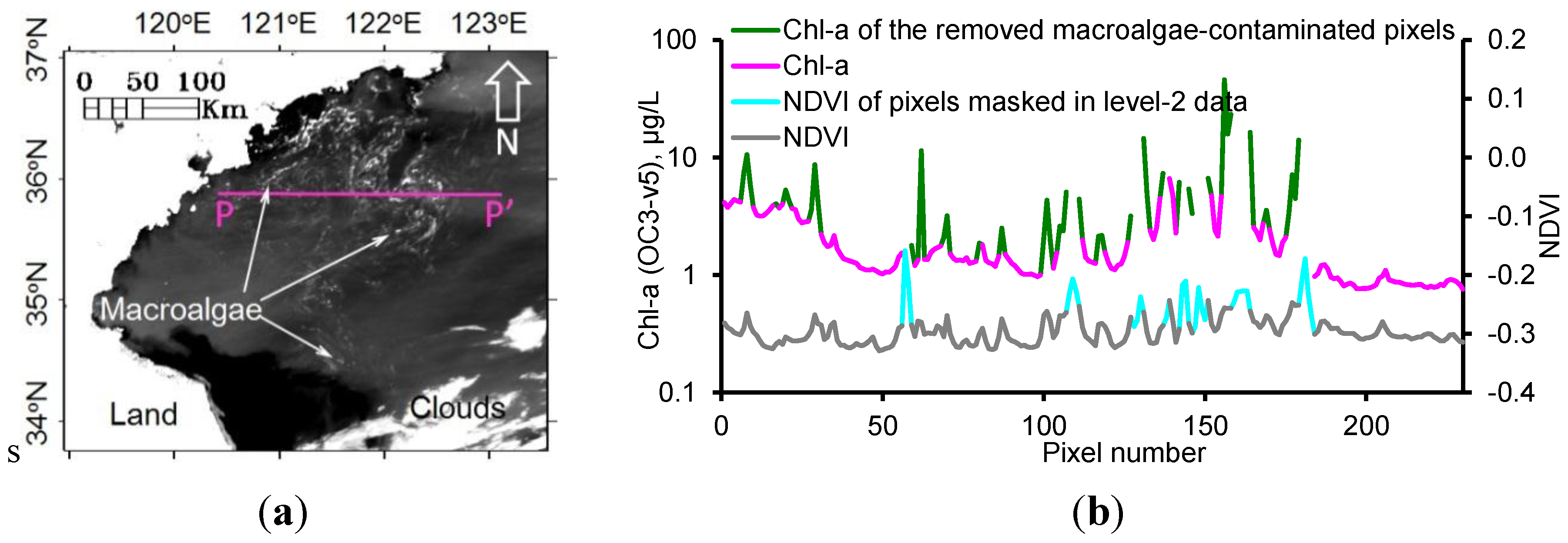
3.1. Impacts of Floating Macroalgae on the Standard MODIS Chl-a Product

Figure 3 and Figure 4 show an example of how the MAB occurrence on 15 July 2009 influenced the standard MODIS Chl-a product. Figure 3b and Figure 4a show that the sea surface was covered by floating macroalgae slicks (white slicks in Figure 4a), and such slicks remained in the MODIS Level-2 composite images although some pixels were flagged as invalid data (black pixels in Figure 3b). The atmospheric correction and Chl-a retrieval algorithms of MODIS aqua were designed for water-column phytoplankton instead of floating macroalgae, and the presence of macroalgae would cause both algorithms to fail, leading to positively-biased Chl-a retrievals (shown by the contrast between Figure 3c,d). The maximum Chl-a derived from MODIS aqua in the macroalgae-contaminated region (Figure 3c) could be as much as 332.89 µg/L. Figure 4b shows clearly how the macroalgae pixels led to overestimation of Chl-a along a transect (P-P’). The Chl-a spikes along the transect were all due to the contamination of the macroalgae pixels, which suggests that the OC3-v5 Chl-a algorithm for phytoplankton was sensitive to the presence of floating macroalgae and thus it might be used as an alternative index for macroalgae pixels, as shown in this study. After the removal of these pixels using a gradient-based method (see the section of data and methods), the mean Chl-a along this transect decreased from 3.19 to 1.70 µg/L. The removal procedure was then used on the Level-2 daily data to exclude the macroalgae-contaminated pixels.
Figure 3. (a) MODIS quasi-true color Red-Green-Blue composite image on 15 July 2009 (R: band 1; G: band 4; B: band 3); (b) color composite image of MODIS Level-2 reflectance: R (Band 7, 2130 nm) G (Band 2, 859 nm) B (Band 1, 645 nm). Light-green slicks show the pixels containing floating macroalgae. (c) Standard Chl-a data product; (d) standard Chl-a data product after the removal of the macroalgae-contaminated pixels. White color indicates land, clouds, and invalid data. All the west-east profiles in pink are the same as the P-P’ line in Figure 3a.
Remotesensing 07 12297 g003
Figure 4. (a) NDVI image corresponding to Figure 3; the white slicks pointed out by arrows are macroalgae; the west-east profile (P-P’) is plotted in pink; (b) NDVI and the Level-2 standard Chl-a along the profile (P-P’). Data gaps in Chl-a indicate the pixels with invalid data flagged as “CHLFAIL” or “CLDICE” in the standard product due to the presence of floating macroalgae.
Remotesensing 07 12297 g004

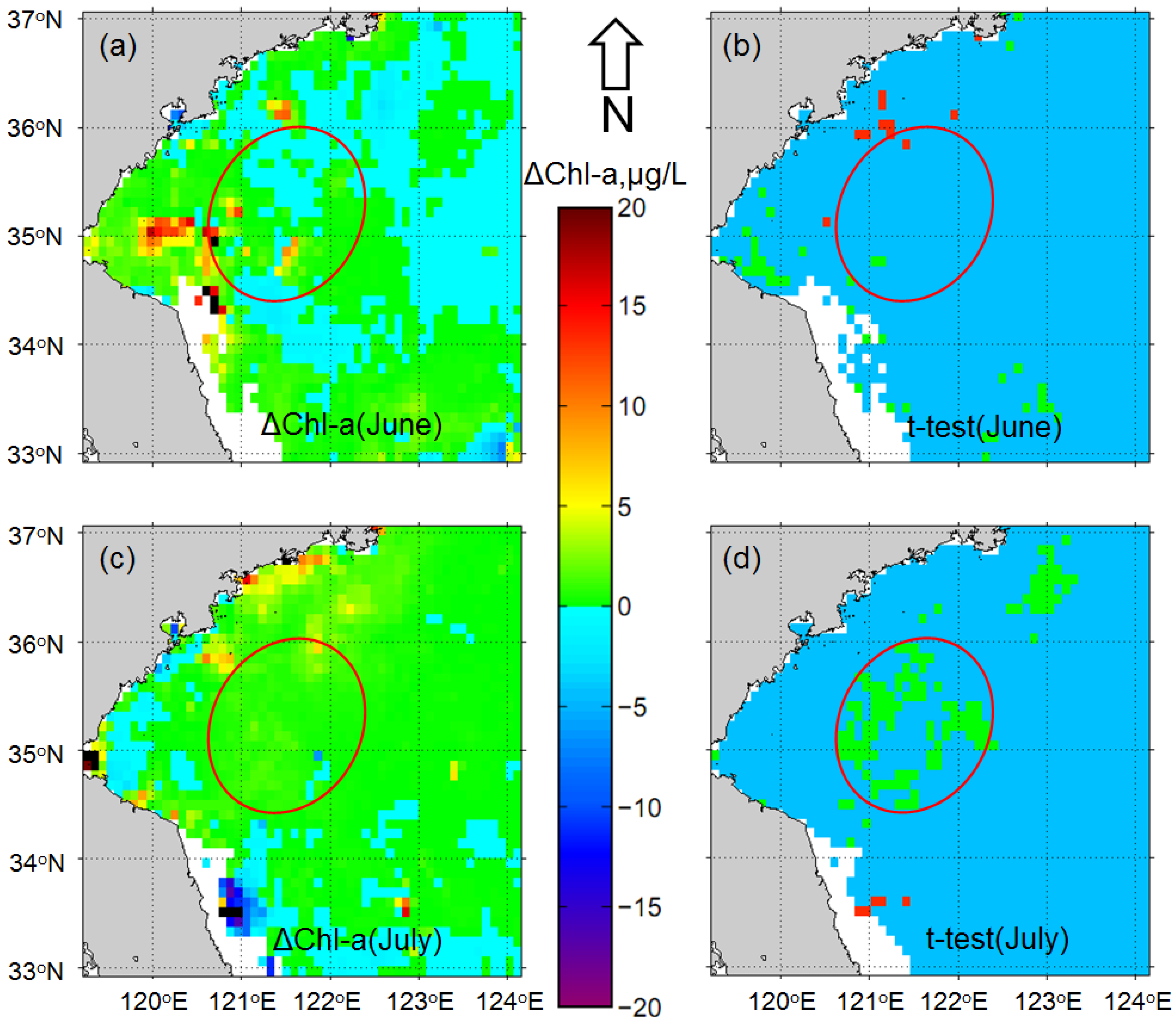
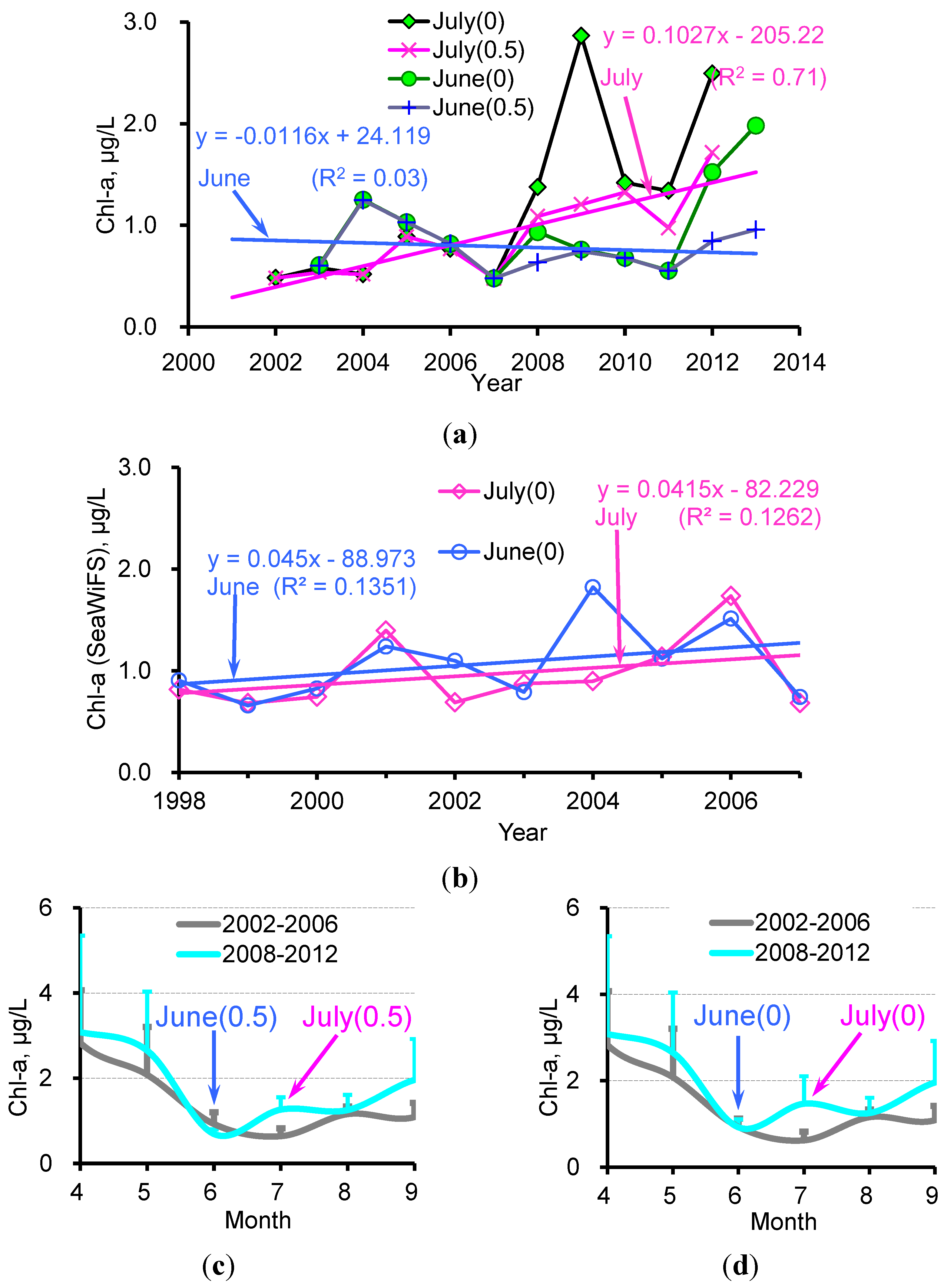
3.2. Monthly Chl-a for June and July after the Removal of Macroalgae-Contaminated Pixels

Figure 5 shows significant increases in the water-column Chl-a for July from the pre-MAB period (2002–2006) to the MAB period (2008–2012), while no significant increases were found for June. The locations with significant increases (p < 0.05) of Chl-a were generally in offshore waters ~50–100 km away from the coasts of the Shandong Peninsula and the Jiangsu Shoal, and these locations (with a coverage of about 9000 km2) were where the MABs occurred (Figure 1).
Figure 6a further shows that during the pre-MAB period Chl-a tended to decrease from June to July, especially in the offshore waters north of the latitude line of 34.5°N. In contrast, during the MAB period Chl-a for July was higher than for June, and some of the Chl-a increases for the MAB region (red circles in Figure 6c,d) were statistically significant.
Figure 7a shows that in the pilot region (Box A in Figure 1, 35.5°N–36°N, 121.25°E–121.75°E, also annotated as the red circle in Figure 6c,d) Chl-a time-series before 2008 (the pre-MAB period) with and without the removal of the macroalgae-contaminated pixels generally overlapped with each other. The significance test (t-test) showed no difference in the average Chl-a between the two time-series in the pilot region in the pre-MAB period. For Chl-a data after 2008 (the MAB period), the removal of the macroalgae pixels led to significantly lower Chl-a for both June and July (t-test), which is in agreement with the results shown in Figure 4b. Such an effect is not apparent in June of 2009, 2010, and 2011 because of less floating macroalgae in this region.
Chl-a data from SeaWiFS showed a linear relationship with those from MODIS, with no statistically significant difference for this study area [6]. A longer time series of SeaWiFS monthly Chl-a (1998–2007, a pre-MAB period) in Figure 7b showed parallel linear trends for July and June (no significant difference between the two slopes, p = 0.95). Comparing these trends of 1998–2007 with those of 2002–2013 (Figure 7a), a shift in the linear trend was found for June, which is coincident with the occurrence of the large-scale MABs.
Figure 5. Changes in the five-year average of the water-column Chl-a for June and July between the pre-MAB period (2002–2006) and the MAB period (2008–2012), generated from the standard level-2 daily Chl-a product after the removal of the macroalgae-contaminated pixels (Figure 3). (a) Difference in Chl-a for June (MAB minus pre-MAB), and (b) significance of the difference. (c) Difference in Chl-a for July (MAB minus pre-MAB) and (d) significance of the difference. Green and red for significant increases and decreases as indicated by t-test (p < 0.05), respectively; blue for non-significant changes; white pixels for no results.
Remotesensing 07 12297 g005
Figure 6. (a) Difference in Chl-a (July minus June) during the pre-MAB period (2002–2006), and (b) significance of the difference. (c) Difference in Chl-a (July minus June) during the MAB period (2008–2012) and (d) significance of the difference. The white dotted line shows the latitude line of 34.5°N. Green and red for significant increases and decreases as indicated by t-test, respectively; blue for non-significant changes; white pixels for no results.
Remotesensing 07 12297 g006
A dramatic difference was found in the June–July Chl-a changes between the pre-MAB period and the MAB period for the pilot region (Figure 7c,d). During the pre-MAB period, the multi-year average of Chl-a for June was 0.92 µg/L, higher than that for July (0.64 µg/L). In contrast, during the MAB period, the multi-year average of Chl-a for June was only 0.69 µg/L, significantly lower (t-test) than that for July (1.26 µg/L). Furthermore, Chl-a for July showed a pronounced linear increasing trend (R2 = 0.71, F-test, p = 0.05) from 2002 to 2013, with a 98% increase from 0.64 µg/L during 2002–2006 to 1.26 µg/L during 2008–2012. In contrast, Chl-a for June showed no significant changes between the two periods. This significant increase of Chl-a for July and low Chl-a for June in the MAB period formed a unique seasonal pattern that was different from the pre-MAB period.
Figure 7. (a) Monthly Chl-a for June and July between 2002 and 2013. The two solid lines show the overall trends for June and July, respectively; (b) SeaWiFS standard monthly Chl-a of June and July before the super macroalgal blooms in the Yellow Sea (pilot region: 35.5°N–36°N, 121.25°E–121.75°E); (c,d) Monthly Chl-a changes for 2002–2006 and 2008–2012 with and without the removal of macroalgae pixels, respectively. Chl-a values for April, May, August, and September were obtained from Level-3 standard MODIS aqua Chl-a products. Vertical bars show the standard deviations (S.D.) of multi-year monthly Chl-a. 0: standard Chl-a with macroalgae included; 0.5: standard Chl-a with macroalgae excluded using a threshold of 0.5 µg/L (see the Methods section for details of data-processing).
Remotesensing 07 12297 g007

4. Discussion

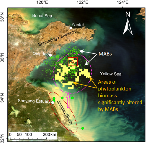
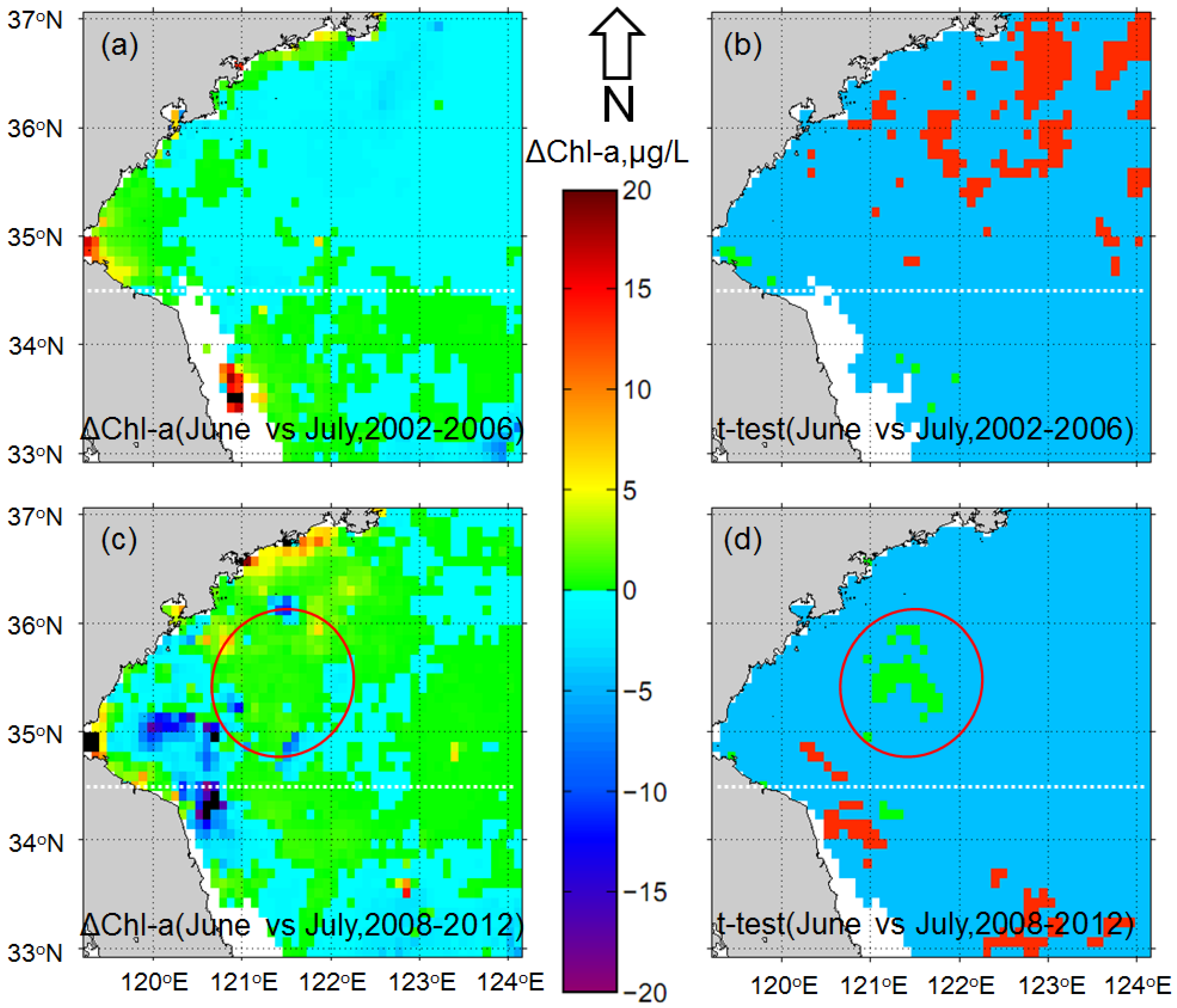
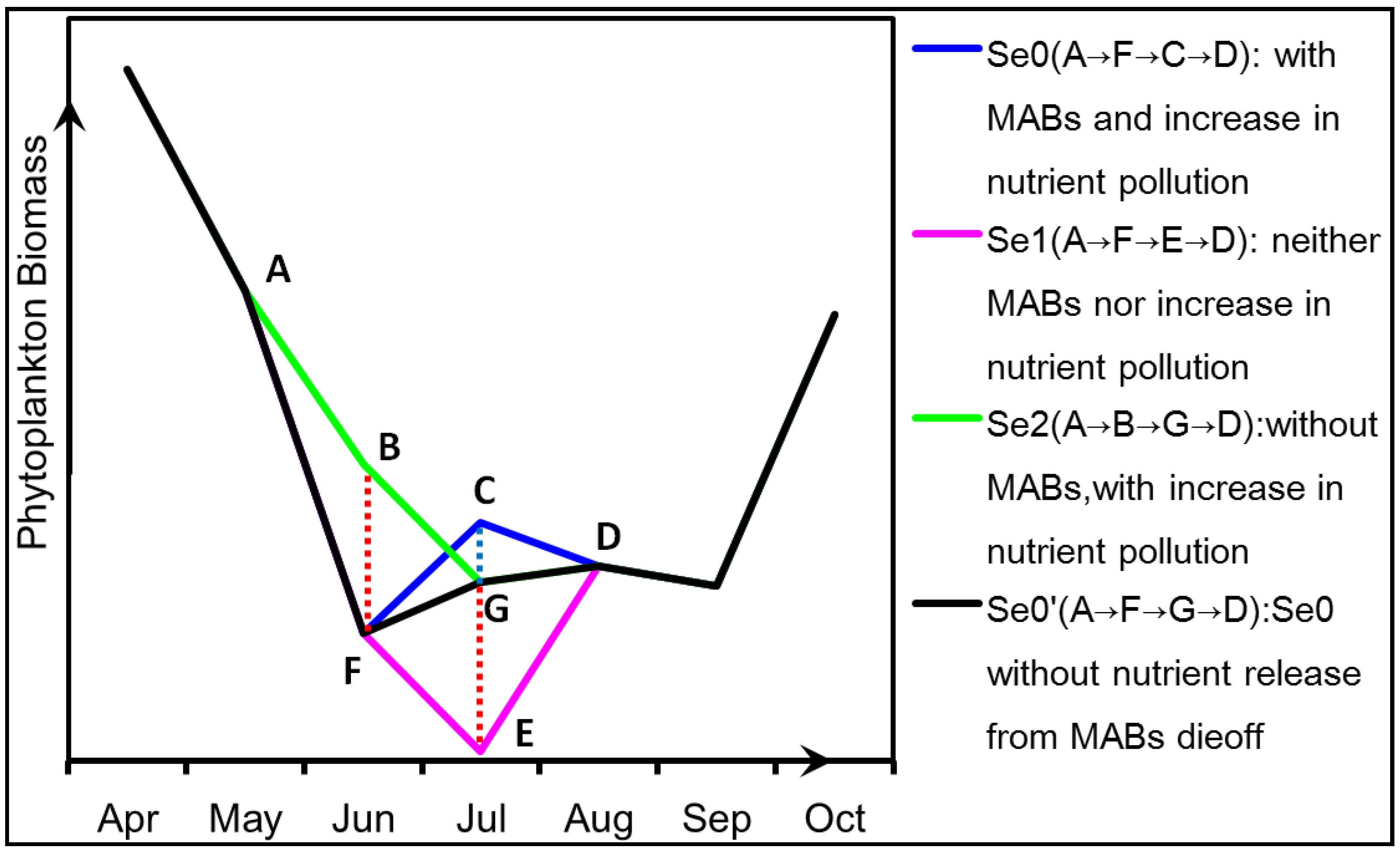
4.1. Increase in Phytoplankton Biomass in the Bloom Region

The NASA standard Chl-a products for the Yellow Sea, after excluding the macroalgae-contaminated pixels, may still contain higher uncertainties than for deep open oceans. The assumption is that the factors (e.g., colored dissolved organic matter) leading to such uncertainties would contribute more or less equally in time, so that the derived temporal or anomaly patterns are still valid, especially when the observed temporal changes are significant. Indeed, the above results indicate significant water-column Chl-a increases from June to July during the MAB period, with or without removal of the macroalgae-contaminated pixels. Such increases were absent during the pre-MAB period. For the Yellow Sea, from May to August, both SST and PAR increased [6]; following these environmental forcing, Chl-a typically peaked in the spring and then decreased monotonically through the fall without an intermediate peak in the summer [27]. The time-series of pre-MAB monthly Chl-a showed such typical patterns, yet the MAB period showed a local peak in July, indicating a shift in phytoplankton phenology. The question, then, is what caused such a shift.
Precipitation over the coastal zone of the Yellow Sea usually peaked in July and August [27], and increased precipitation may bring more land-based nutrients to the Yellow Sea to fuel the phytoplankton in coastal waters. However, in this study, the locations with significant Chl-a increases were generally in offshore waters far away from land (Figure 5d), suggesting that precipitation was an unlikely reason. Neither SST nor PAR showed pronounced shifts for June and July (Figure 8a,b); they may therefore be ruled out as possible causes of the observed Chl-a changes from the pre-MAB period to the MAB period.
The Jiangsu Shoal has served as a pool of nutrient supply (e.g., the DIN and PO4-P) and macroalgae seed to the Yellow Sea [4,6,8,9]. Xia et al. [28] showed that the surface DIN and the PO4-P concentrations during 7–14 July 2008 in the Jiangsu coastal waters were higher by a factor of 2 than those in the bloom region in the Yellow Sea. Expansion of local aquaculture as well as river input has caused rapid increases in nutrient supplies in the Jiangsu Shoal [29]. Figure 8c shows that the Jiangsu coastal waters may contribute as much as 80% of the water quality pollution to the entire Yellow Sea. Indeed, even when nutrient pollution decreased in other nearshore regions, Jiangsu coastal waters still showed increases in nutrient pollution, suggesting a significant nutrient source to the Yellow Sea.
Xing et al. [6] revisited the progressive eutrophication in the Yellow Sea and the Jiangsu Shoal, and suggested that the process of progressive eutrophication might contribute to the non-linear sudden outburst of MABs since 2007 [4,9]. In summer, under the influence of southeast wind and local circulations [5,8,10], surface waters from the Jiangsu Shoal could flow northward and stimulate macroalgae growth in the Yellow Sea (please see Supplement II for sea surface currents). Thus, increased nutrient supply from the Jiangsu Shoal fueled not only the macroalgae but also the water-column phytoplankton in summer. The monthly Chl-a for June peaked in 2004 in the offshore waters of the Yellow Sea to the south of the Shandong Peninsula (pilot region, box A in Figure 1), indicating a response to the high-level nutrient supply from the Jiangsu Shoal in 2004 (Figure 8d). The increased nutrient supply in the Jiangsu Shoal could also explain the significant Chl-a increases in July from the pre-MAB period to the MAB period. Yet, it could not explain why a similar increase was not observed for the month of June. A nutrient budget is required to explain such a difference.
Figure 8. (a) Monthly sea surface temperature (SST) and (b) photosynthetically active radiation (PAR) for June and July during the 2000–2013 period in the pilot region (box A in Figure 1); there is no statistically significant difference between SeaWiFS and MODIS data for the overlapping period. (c) Unclean waters (mainly nutrient polluted waters with water quality levels II, III, IV, and V) in the Jiangsu Shoal (JSS) and the Yellow Sea (YS) during the 2003–2011 period [6]; “YS-JSS” represents the annual area of unclean waters of the YS excluding that of the JSS; “JSS:YS” represents the ratio of unclean waters of the JSS to that of the YS. (d) Level-3 standard MODIS aqua and terra Chl-a for June in the pilot region versus the annual average of nutrient concentrations in the JSS [6].
Remotesensing 07 12297 g008

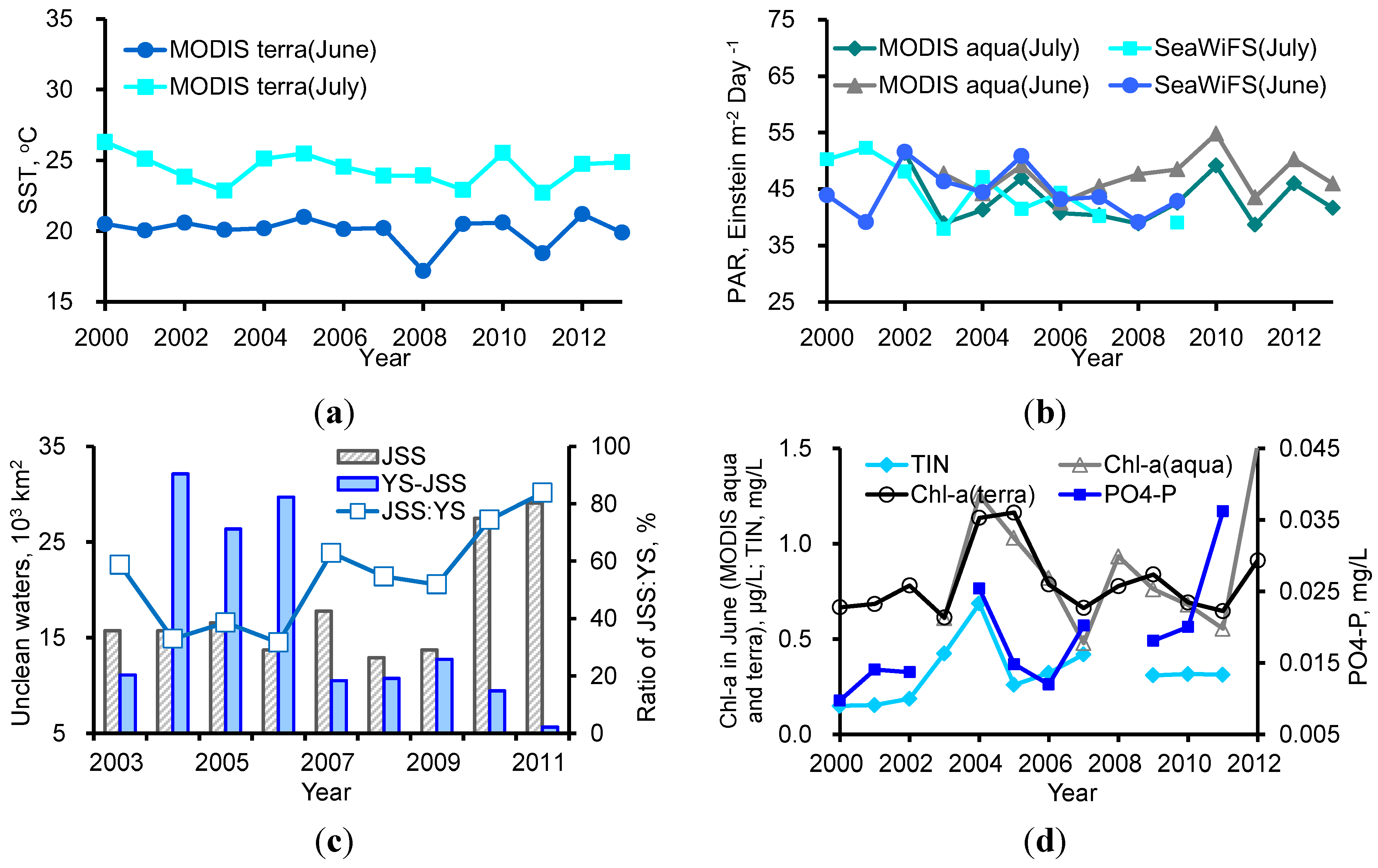
4.2. Nutrient Competition between Macroalgae and Phytoplankton

In theory, nutrient competition between macroalgae and phytoplankton could have occurred with the emergence of such large-scale MABs in the Yellow Sea. The limited in situ data, when combined with the satellite time series of Chl-a, may be used to evaluate the nutrient competition on the basis of mass balance.
It has been hypothesized that the increases in nutrient supply from the pre-MAB period (2002–2006) to the MAB period (2008–2012) could lead to the Chl-a increases in July between the two periods [6]. No increases of Chl-a in June could be due to the consumption of large amounts of nutrients by the macroalgae during their initial growth. In the following month of July during the MAB period, nutrients from the Jiangsu Shoal and potentially those recycled from macroalgae to the water column might lead to the observed increases in Chl-a. Such a hypothesis is illustrated in the schematic chart in Figure 9, where the sequence of AFCD shows the situation for June and July during the MAB period (i.e., with increased nutrient supply and occurrence of MABs), and the sequence of AFED shows a scenario with neither increases in nutrient supply nor occurrence of MABs. The sequence of ABGD shows a scenario with increases in nutrient supply but without occurrence of MABs, and the sequence of AFGD shows increases in nutrient supply and occurrence of MABs but without nutrient release from macroalgae to the water column. The following estimates may support this hypothesis.
Figure 9. Schematic chart showing scenarios of how phytoplankton biomass could be modulated by nutrient supplies and MABs in the May–August period. Se0 (A→F→C→D): the real situation (2008–2012) with MABs and increased nutrient supply; Se1 (A→F→E→D): without increases in nutrient supply and occurrence of MABs; Se2 (A→B→G→D): without occurrence of MABs but with increases in nutrient supply; Se0’(A→F→G→D): the same as scenario Se0 but without nutrient release from macroalgae to the water column in July. Nutrients of phytoplankton biomass (BF) correspond to those consumed by macroalgae in June, and biomass (CG) corresponds to the potential nutrients released from macroalgae die-off for July.
Remotesensing 07 12297 g009
The prevailing growth month of MABs in the open waters of the Yellow Sea was usually June. Table 1 shows that massive floating macroalgae usually landed on the beaches of Qingdao (see Figure 1 and Figure 3) near the end of June, indicating that massive MABs occurred in the offshore waters of the Yellow Sea in June (Figure 1).
Table 1. Initial landing date of macroalgae on Qingdao beaches.
Year (yyyy)20082009 *201020112012201320142015 *
Landing date (day/month)28/614/727/66/728/630/628/61/7
During summer 2008, when the record-high MABs were reported, one million tons of macroalgae (wet weight, Mm∙ww) were collected [7,9], and about 40,000 km2 of the sea’s surface were impacted [6,8]. According to [30], nitrogen in macroalgae (Cm∙N) was about 1.5% of the dry weight. From our own investigation in summer 2014, the ratio of wet weight of macroalgae to dry weight (Rm∙wd) was about 5. Therefore, one million tons of macroalgae were equivalent to about 3000 tons of nitrogen (Mm∙N). It should be noted that there should be large amounts of macroalgae landed in other sites of the Shandong Peninsula or sunk to the sea bottom. Thus, the total macroalgae biomass and the corresponding nitrogen based on collection in Qingdao alone must have been underestimated.
With the occurrence of MABs, a decrease of 0.5 µg/L in Chl-a (DChl-a) during June (a conservative estimate, as shown in Figure 3c and Figure 4f) would be expected from the 2002–2006 period to the 2008–2012 period. For the surface layer (10 m, a maximum Secci Disk depth in this region) in a given area of 9000 km2 and under the simplified uniform conditions: 1 µg/L Chl-a corresponds to 130 µg/L phytoplankton biomass (dry weight), and nitrogen content in phytoplankton (dry weight) is about 3% (http://www.cee.pdx.edu/w2/), a decrease of 0.5 µg/L in Chl-a would correspond to a decrease of phytoplankton biomass and a decrease of 175.5 tons of nitrogen. Considering the deposition of phytoplankton and a turnover (TO) cycle of three days, there should be a loss of nutrient supply of 1755 tons of nitrogen for phytoplankton (Mp∙N) for the whole month of June, which is on the same order as that consumed by macroalgae (3000 tons of nitrogen) during the same period. So, these arguments support the hypothesis that there might be significant nutrient competition between floating macroalgae and phytoplankton for this region. Table 2 gives a summary of this mass balance for nitrogen.
Table 2. Nitrogen estimation for macroalgae-phytoplankton nutrient competition.
MacroalgaePhytoplankton
Mm∙ww, biomass (wet weight), kg: 1 × 10⁹
Rm∙wd, ratio of wet weight to dry weight: 5
Cm∙N, nitrogen content, % (dry weight): 1.5
A, area with decrease of Chl-a, km2: 9 × 10³
WD, water depth with decrease of Chl-a, m: 10
DChl-a, decrease of Chl-a, mg/m3: 0.5
Rbc, ratio of biomass (dry weight) to Chl-a: 130
Cp∙N, nitrogen content, % (dry weight): 3
TO, turn over cycles in a month: 10
Mm∙N, nitrogen in macroalgae, kg: 3 × 10⁶
(Mm∙N = Mm∙ww × (Cm∙N/100)/Rm∙wd)
Mp∙N, nitrogen in phytoplankton, kg: 1.755 × 10⁶
(Mp∙N = A × WD × DChl-a × Rbc × (Cp∙N/100) × TO)

5. Conclusions

The world’s largest MABs have occurred in the Yellow Sea every summer since 2008, but their impacts on water-column phytoplankton biomass have never been documented. Using MODIS aqua Chl-a data products, we presented the first report that the MABs reduced water-column phytoplankton biomass through nutrient competition in the Yellow Sea in June. In this study, any pixel with its Chl-a 0.5 µg/L larger than the mean Chl-a of a window of 9 × 9 pixels around it was regarded as a macroalgae-contaminated pixel and removed from the daily Level-2 standard MODIS aqua Chl-a data to generate a new time series of Chl-a (an index of water-column phytoplankton biomass). The new data show that, in the offshore Yellow Sea frequently visited by MABs, there were no significant changes in Chl-a in June from the pre-MAB period (2002–2006) to the MAB period (2008–2012); in contrast, Chl-a in July significantly increased in an area of about 9000 km2. The two different changing patterns in Chl-a for June and July, respectively, suggest a significant decrease in phytoplankton biomass due to the nutrients’ consumption in June with increased macroalgae biomass.
While the findings here can be explained with the nutrient hypothesis, they are preliminary in nature. In particular, the uncertainties of the NASA standard Chl-a (after removal of the macroalgae-contaminated pixels) in the study region need to be quantified and reduced with field data. Finally, when applying the approach to other sensors with different resolutions, the window size used to remove macroalgae-contaminated pixels may also need to be adjusted.

Supplementary Files

Supplementary File 1

Acknowledgments

This work was supported by projects from the Chinese Academy of Sciences (Nos. XDA11020403, XDA11020102, KZCX2-YW-Q07-01), the CAS/SAFEA International Partnership Program for Creative Research Teams, the INTER-GOVERNMENTAL S&T COOPERATION (China-Romania), and the University of South Florida. We especially thank the Institute of Oceanology, Chinese Academy of Sciences for organizing the open cruise in the Yellow Sea, and Yanju Hao, Xiangyang Zheng, and Xiaojuan Tian for performing the field sampling, data collection, and simulation. Thanks to Julie Kesby (PEMS, UNSW Canberra) for editorial advice on this paper.

Author Contributions

Qianguo Xing conceived the study; Qianguo Xing, Chuanmin Hu and Danling Tang performed the study and analyzed the data; Shilin Tang and Mingjing Lou processed satellite image, Liqiao Tian collected the data; Xuelu Gao and Xiao Hua Wang reviewed the nutrient transportation. Qianguo Xing and Chuanmin Hu prepared the manuscript, and all authors discussed the results and commented on the manuscript.

Conflicts of Interest

The authors declare no conflict of interest.

References

  1. Smetacek, V.; Zingone, A. Green and golden seaweed tides on the rise. Nature 2013, 504, 84–88. [Google Scholar] [CrossRef] [PubMed] [Green Version]
  2. Lyons, D.A.; Arvanitidis, C.; Blight, A.J.; Chatzinikolaou, E.; Guy-Haim, T.; Kotta, J.; Orav-Kotta, H.; Queiros, A.M.; Rilov, G.; Somerfield, P.J.; et al. Macroalgal blooms alter community structure and primary productivity in marine ecosystems. Glob. Chang. Biol. 2014, 20, 2714–2724. [Google Scholar] [CrossRef] [PubMed]
  3. Hu, C.; He, M.X. Origin and offshore extent of floating algae in Olympic sailing area. Eos Trans. AGU 2008, 89, 302–303. [Google Scholar] [CrossRef]
  4. Hu, C.; Li, D.; Chen, C.; Ge, J.; Muller-Karger, F.E.; Liu, J.; Yu, F.; He, M. On the recurrent Ulva Prolifera blooms in the Yellow Sea and East China Sea. J. Geophys. Res. 2010, 115. [Google Scholar] [CrossRef]
  5. Xing, Q.; Loisel, H.; Schmitt, F.; Shi, P.; Liu, D.; Keesing, J. Detection of the green tide at the Yellow Sea and tracking its wind-forced drifting by remote sensing. In Proceedings of the 2009 EGU General Assembly, Vienna, Austria, 19–24 April 2009.
  6. Xing, Q.; Tosi, L.; Braga, F.; Gao, X.; Gao, M. Interpreting the progressive eutrophication behind the world’s largest macroalgal blooms with water quality and ocean color data. Nat. Hazards 2015, 78, 7–21. [Google Scholar] [CrossRef]
  7. Wang, X.; Li, L.; Bao, X.; Zhao, L. Economic cost of an algae bloom cleanup in China’s 2008 Olympic sailing venue. Eos Trans. AGU 2009, 90, 238–239. [Google Scholar] [CrossRef]
  8. Liu, D.; Keesing, J.K.; Xing, Q.; Shi, P. World’s largest macroalgal bloom caused by expansion of seaweed aquaculture in China. Mar. Pollut. Bull. 2009, 58, 888–895. [Google Scholar] [CrossRef] [PubMed]
  9. Xing, Q.; Zheng, X.; Shi, P.; Hao, J.; Yu, D.; Liang, S.; Liu, D.; Zhang, Y. Monitoring “Green Tide” in the Yellow Sea and the East China Sea using multi-temporal and multi-source remote sensing images. Spectrosc. Spect. Anal. 2011, 31, 1644–1647. (in Chinese). [Google Scholar]
  10. Zheng, X.; Xing, Q.; Shi, P.; Li, L. Numerical simulation of the 2008 green tide in the Yellow Sea. Mar. Sci. 2011, 35, 82–87. [Google Scholar]
  11. Smith, D.W.; Horne, A.J. Experimental measurement of resource competition between planktonic microalgae and macroalgae (seaweeds) in mesocosms simulating the San Francisco Bay-Estuary, California. Hydrobiologia 1988, 159, 259–268. [Google Scholar] [CrossRef]
  12. Fong, P.; Donohoe, R.M.; Zedler, J.B. Competition with macroalgae and benthic cyanobacterial mats limits. Mar. Ecol. Prog. Ser. 1993, 100, 97–102. [Google Scholar] [CrossRef]
  13. Sfriso, A.; Pavoni, B. Macroalgae and phytoplankton competition in the central Venice Lagoon. Environ. Tech. 1994, 15, 1–14. [Google Scholar] [CrossRef]
  14. Tang, D.; Kawamura, H.; Doan-Nhu, H.; Takahashi, W. Remote sensing oceanography of a harmful algal bloom (HAB) off the coast of Southeastern Vietnam. J. Geophys. Res. Oceans 2004, 109. [Google Scholar] [CrossRef]
  15. Tang, D.; Kawamura, H.; Sang Oh, I.; Baker, J. Satellite evidence of harmful algal blooms and related oceanographic features in the Bohai Sea during autumn 1998. Adv. Space Res. 2006, 37, 681–689. [Google Scholar] [CrossRef]
  16. Cui, T.; Zhang, J.; Sun, L.; Jia, Y.; Zhao, W.; Wang, Z.; Meng, J. Satellite monitoring of massive green macroalgae bloom (GMB): Imaging ability comparison of multi-source data and drifting velocity estimation. Int. J. Remote Sens. 2012, 33, 5513–5527. [Google Scholar] [CrossRef]
  17. Shi, W.; Wang, M. Green macroalgae blooms in the Yellow Sea during the spring and summer of 2008. J. Geophys. Res. Oceans 2009, 114. [Google Scholar] [CrossRef]
  18. Edelvang, K.; Kaas, H.; Erichsen, A.C.; Alvarez-Berastegui, D.; Bundgaard, K.; Jugensen, P.V. Numerical modelling of phytoplankton biomass in coastal waters. J. Mar. Syst. 2005, 57, 13–19. [Google Scholar] [CrossRef]
  19. Ma, J.; Zhan, H.; Du, Y. Seasonal and interannual variability of surface CDOM in the South China Sea associated with El Niño. J. Mar. Syst. 2011, 85, 86–95. [Google Scholar]
  20. Liu, C.; Tang, D. Spatial and temporal variations in algal blooms in the coastal waters of the western South China Sea. J. Hydrol. Environ. Res. 2012, 6, 239–247. [Google Scholar] [CrossRef]
  21. Miller, R.L.; López, R.; Mulligan, R.P.; Reed, R.E.; Liu, C.C.; Buonassissi, C.J.; Brown, M.M. Examining material transport in dynamic coastal environments: An integrated approach using field data, remote sensing and numerical modeling. In Remote Sensing and Modeling: Advances in Coastal and Marine Resources Coastal Research Library; Finkl, C.W., Makowski, C., Eds.; Springe: New York, NY, USA, 2014; pp. 333–364. [Google Scholar]
  22. Dien, T.V.; Tang, D.; Kawamura, H. Validation SeaWiFS-Derived ocean color data and using for study distribution chlorophyll-a concentration in the Vietnam waters. In Proceedings of the 2003 Regional Conference on Digital GMS, Bangkok, Thailand, 26–28 February 2003; pp. 75–87.
  23. Nagamani, P.V.; Hussain, M.I.; Choudhury, S.B.; Panda, C.R.; Sanghamitra, P.; Kar, R.N.; Das, A.; Ramana, I.V.; Rao, K.H. Validation of chlorophyll-a algorithms in the coastal waters of Bay of Bengal initial validation results from OCM-2. J. Indian Soc. Remote Sens. 2013, 41, 117–125. [Google Scholar] [CrossRef]
  24. Kahru, M.; Kudela, R.M.; Anderson, C.R.; Manzano-Sarabia, M.; Mitchell, B.G. Evaluation of satellite retrievals of ocean Chlorophyll-a in the California Current. Remote Sens. 2014, 6, 8524–8540. [Google Scholar] [CrossRef]
  25. Li, G.; Gao, P.; Wang, F.; Liang, Q. Estimation of ocean primary productivity and its spatio-temporal variation mechanism for East China Sea based on VGPM model. J. Geogr. Sci. 2004, 14, 32–40. [Google Scholar] [CrossRef]
  26. Shi, W.; Wang, M. Satellite views of the Bohai Sea, Yellow Sea, and East China Sea. Prog. Oceanogr. 2012, 104, 30–45. [Google Scholar] [CrossRef]
  27. Xing, Q.; Loisel, H.; Schmitt, F.G.; Dessailly, D.; Hao, Y.; Han, Q.; Shi, P. Fluctuations of satellite-derived chlorophyll concentrations and optical indices at the Southern Yellow Sea. Aquat. Ecosyst. Health Manag. 2012, 15, 168–175. [Google Scholar]
  28. Xia, B.; Ma, S.; Cai, Y.; Chen, B.; Chen, J.; Song, Y.; Mao, Y. Distribution of temperature, salinity, dissolved oxygen, nutrients and their relationships with green tide in Enteromorpha prolifera outbreak area of the Yellow Sea. Progr. Fish. Sci. 2009, 30, 94–101. (In Chinese) [Google Scholar]
  29. Liu, F.; Pang, S.; Chopin, T.; Gao, S.; Shan, T.; Zhao, X.; Li, J. Understanding the recurrent large-scale green tide in the Yellow Sea: Temporal and spatial correlations between multiple geographical, aquacultural and biological factors. Mar. Environ. Res. 2013, 83, 38–47. [Google Scholar] [CrossRef] [PubMed]
  30. Zhao, Y.; Ning, J.; Shang, D.; Zhai, Y. Analysis of inorganic elements of Enteramorpha prolifera from Qingdao coasts in 2008. J. Biol. 2010, 27, 92–93. (In Chinese) [Google Scholar]

