Article

Assessment of Image-Based Point Cloud Products to Generate a Bare Earth Surface and Estimate Canopy Heights in a Woodland Ecosystem

by
Jennifer L. R. Jensen
1,* and
Adam J. Mathews
2
1
Department of Geography, Texas State University, 601 University Drive, San Marcos, TX 78666, USA
2
Department of Geography, Oklahoma State University, 337 Murray Hall, Stillwater, OK 78078, USA
*
Author to whom correspondence should be addressed.
Submission received: 4 November 2015 / Revised: 30 December 2015 / Accepted: 31 December 2015 / Published: 8 January 2016

Abstract

:
We examine the utility of Structure from Motion (SfM) point cloud products to generate a digital terrain model (DTM) and estimate canopy heights in a woodland ecosystem in the Texas Hill Country, USA. Very high spatial resolution images were acquired with a Canon PowerShot A800 digital camera mounted on an unmanned aerial system. Image mosaicking and dense point matching were accomplished using Agisoft PhotoScan. The resulting point cloud was classified according to ground/non-ground classes and used to interpolate a high resolution DTM which was both compared to a DTM from an existing lidar dataset and used to model vegetation height for fifteen 20 × 20 m plots. Differences in the interpolated DTM surfaces demonstrate that the SfM surface overestimates lidar-modeled ground height with a mean difference of 0.19 m and standard deviation of 0.66 m. Height estimates obtained solely from SfM products were successful with R2 values of 0.91, 0.90, and 0.89 for mean, median, and maximum canopy height, respectively. Use of the lidar DTM in the analyses resulted in R2 values of 0.90, 0.89, and 0.89 for mean, median, and maximum canopy height. Our results suggest that SfM-derived point cloud products function as well as lidar data for estimating vegetation canopy height for our specific study area.

Graphical Abstract

1. Introduction

Over the past 15 years, our ability to characterize and quantify vegetation structure has been greatly augmented by the use of three dimensional data obtained from light detection and ranging (lidar) sensors. The use of lidar data has allowed for improved estimates and representations of vegetation canopy height [1,2], canopy cover [3,4], leaf area index (LAI) [5,6,7], biomass [8,9,10] and other biophysical variables. In short, lidar data have allowed for significant improvements in many areas of topographic representations and vegetation structure modeling, especially when compared to the sole application of passive multispectral sensors [6,11,12,13]. However, the cost of lidar data can be prohibitive for many applications, especially when the study area is relatively small or requires repeat acquisitions to monitor vegetation change.
Within the past several years, an increasing number of studies have been published that examine the use of Structure from Motion (SfM) to generate products more traditionally associated with lidar datasets. SfM is a computer vision technique that can generate high density three dimensional point clouds from high resolution imagery acquired from multiple perspectives [14]. More frequently, these images are acquired from relatively low-cost unmanned aerial system (UAS) platforms. SfM is similar to traditional photogrammetry in that the technique uses overlapping images to construct dense three-dimensional point clouds of a surface, yet SfM differs from traditional photogrammetry due to the ability of the image matching algorithms to recognize conjugate features in randomly acquired images that exhibit significant variability in spatial resolution and perspectives [15]. For a full review of the SfM technique, the reader is referred to [16,17].
The utility of SfM to generate image-based point clouds is gaining recognition as a low-cost alternative for, or to augment, existing lidar datasets. UAS-acquired imagery and corresponding point clouds are gaining recognition in the literature as their utility spans diverse applications including digital preservation and representation of urban and cultural features [17,18,19,20], archaeology [21], and digital terrain modeling (digital terrain model; DTM) [15,22]. However, to date, few studies have been published in regard to vegetation modeling, an area of research and application that often requires repeat data acquisitions to monitor trajectories of change.
A pioneer study by Dandois and Ellis [23] used image-based point clouds to generate tree canopy height models for two 2.25 ha test sites, compared the models with in situ observations, and were able to account for 64 percent of field measured variability. In their 2010 study, Dandois and Ellis [23] used an existing lidar dataset to serve as the DTM from which to base vegetation heights. In a more recent study, Dandois and Ellis [22] generated 3D forest mapping products that favorably compared with lidar-derived estimates, and more importantly, were able to do so with SfM-based terrain models. Additionally, Mathews and Jensen [24] implemented high density SfM point cloud products to generate DTM and canopy density models to estimate vineyard canopy LAI with moderate success (R2 = 0.57). The generation of accurate DTMs under vegetation canopy is of particular interest since one of the cited drawbacks of image-based point clouds is the reliance on existing lidar data to provide an accurate terrain surface [25].
Although lidar data sets are increasingly available through governmental and non-profit agencies, coverage is still lacking in many areas where fine-scale terrain products and vegetation modeling are needed. Research that addresses the utility and effectiveness of low-cost imagery and associated point clouds is necessary to demonstrate under what landscape conditions these methods are applicable. The objectives of our study were to: (1) compare digital terrain products generated from a SfM-derived point cloud and a previously acquired lidar dataset; and (2) evaluate the utility of SfM-derived point cloud products to estimate tree canopy height in an oak-juniper woodland ecosystem using both the DTMs created from the SfM process and an existing lidar dataset.

2. Materials and Methods
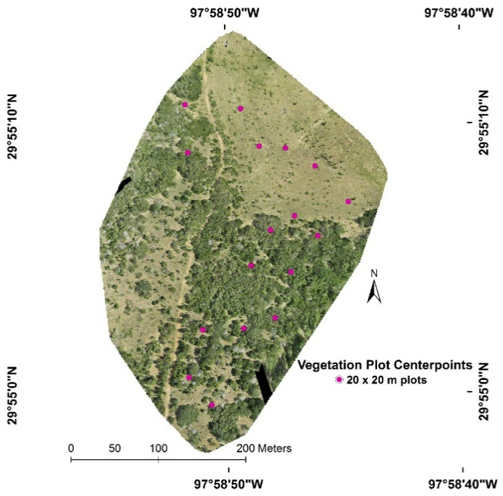
2.1. Study Area

Our study was conducted over approximately 15 ha on a portion of Freeman Center, a Texas State University managed resource on the Edwards Plateau in Central Texas (29°55’8.27″N, 97°58’44.52″W, Figure 1). Study area elevation varies between 204 and 287 m and consists of level terrain to undulating hills. Vegetation composition is characterized by Plateau Live Oak (Quercus virginiana var. fusiformis)-Ashe juniper (Juniperus ashei) savannah that transitions to closed canopy woodlands at lower elevations. Understory vegetation consists of various cool- and warm season grasses, forbs, and sedges in addition to woody shrubs such as Texas persimmon (Diospyron texana), Agarita (Berberis trifoiolata), and Elbow bush (Foresteria pubescens).

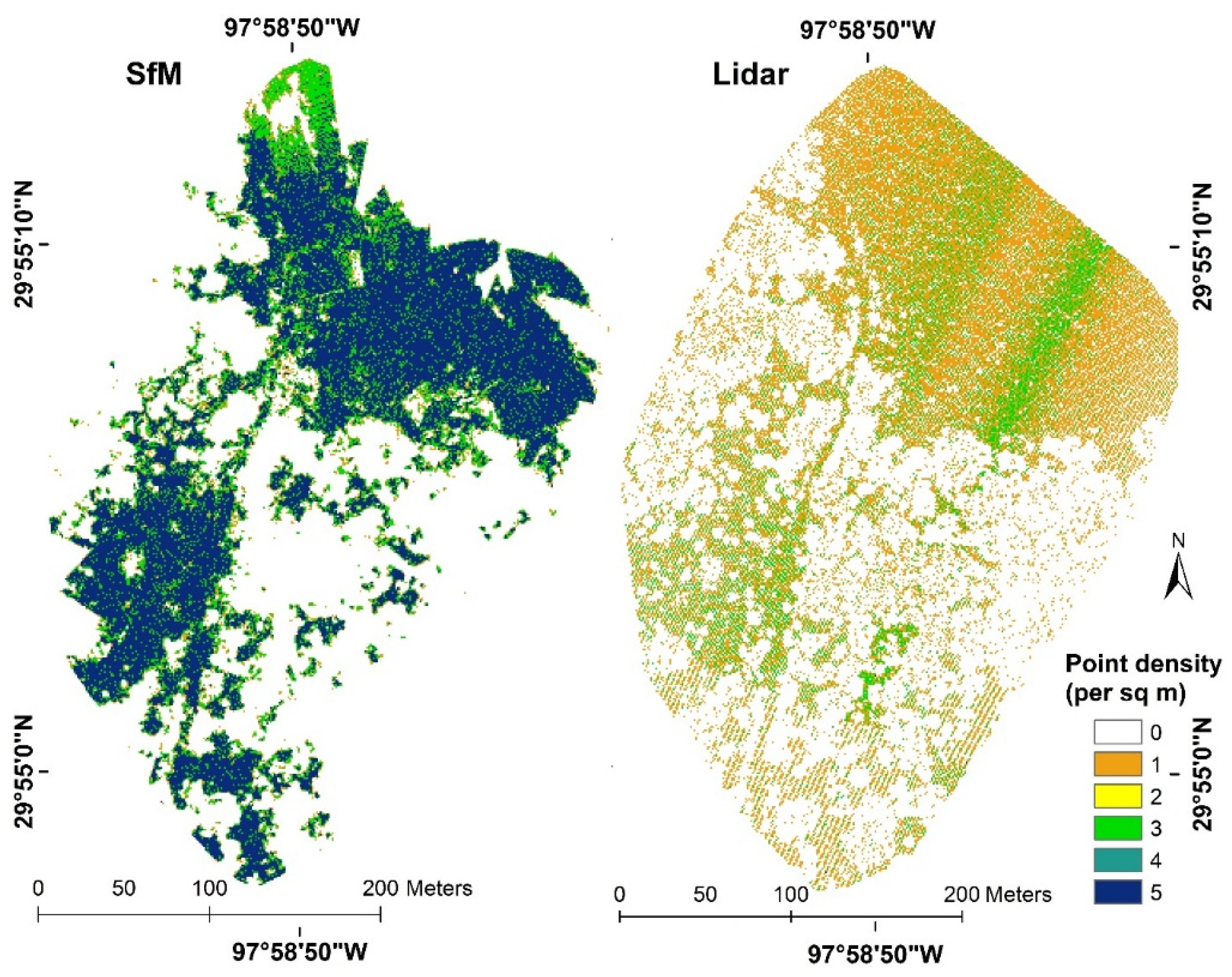
2.2. Image Data Collection, Processing, and Point Cloud Generation

Images were collected during full-canopy, leaf-on conditions, and cloud-free sky on 14 August 2013 from approximately 12:15 pm to 12:45 pm to minimize the effect of shadowing. Two separate flights (each about 12 min coinciding with battery life) resulted in a total of 1166 images of the study site to ensure adequate coverage and overlap for the SfM-derived image mosaic and subsequent dense-point matching. Individual images were captured using a manually remote controlled Hawkeye II UAS (www.ElectricFlights.com, Kingsland, TX, USA). The Hawkeye is a kitewing plane with a sufficient payload to mount two nadir-facing digital cameras simultaneously (approximately 500 g total). Flight paths were oriented north-to-south to fly directly into (south) and with (north) the wind. This was necessary due to the UAS being susceptible to wind gusts. Winds were desirably low (around 15 kph) upon data capture. Flying height averaged approximately 100 m resulting in imagery with a nominal spatial resolution of 5 cm.
Figure 1. SfM-generated orthomosaic from UAV-acquired images for the 15 ha study area. Pink dots represent the of the 20 × 20 m vegetation measurement plots.
Remotesensing 08 00050 g001
Two off-the-shelf Canon PowerShot A800 digital cameras captured images every second throughout the flights using a Canon Hackers Development Kit (CHDK; chdk.wikia.com) intervalometer script preloaded onto the camera SD cards. Most images were captured at nadir, but many were captured with oblique perspectives. The cameras captured oblique images when purposely banked by the remote control operator or when inadvertently banked due to easterly or westerly (side-to-side) wind gusts. These oblique images were not removed from data processing because, in SfM-based product generation, increased number of angles/perspectives is encouraged [23].
To georeference the SfM mosaic to a projected coordinate system, eight ground control points (GCPs) were placed in the field prior to image capture. All GCP targets were crafted out of inexpensive, reusable sturdy foam board. Five of these targets were square, sized 0.6 m × 0.6 m, and painted bright red with small concentric black and white circles at the center following [26]. The remaining three targets were circular with diameters of 0.15 m and were painted only bright red. These bright colors made for high contrast and easy identification of GCPs in resulting images. These distinct colors and shapes, compared to the surrounding natural landscape, found within many images facilitated SfM keypoint matching. The targets were placed throughout the study area to provide adequate coverage and account for variability in terrain elevation. All of the GCP targets were GPS located using a Trimble GeoXH with external Zephyr antenna. A total of 200 positions were collected and averaged to geolocate each GCP (X,Y: NAD83, UTM Zone 14N; and Z: NADV88). All GPS data were differentially corrected after collection using the Trimble GPS Analyst Extension in ArcGIS. Ground target data exhibited a mean estimated error of <15 cm.
The SfM-derived point cloud was created automatically using Agisoft PhotoScan (Agisoft LLC, St. Petersburg, Russia). Of the total 1166 UAS-collected images, 361 were input to first create the SfM image mosaic and then execute the dense point matching. This subset of images was selected based primarily on image clarity, altitude, and area imaged. Since PhotoScan creates an arbitrarily-located point cloud (i.e., Cartesian coordinates), the point cloud needed to be manually georeferenced using the known positions of the GCP targets. As such, each of the GCPs were identified within the PhotoScan generated point cloud and the known UTM coordinates were input to replace the arbitrary ones. Upon completion, PhotoScan transformed the entire point cloud to the known coordinates and optimized its image alignment.
Prior to export, noise in the form of outlier points with extreme high and extreme low elevation values were removed. Noise removal with SfM datasets is not uncommon [22,24]. Finally, to reduce the total number of points and allow point cloud classification to remain a manageable task, the point cloud was exported to LAS format using the dense-low quality setting in PhotoScan.

2.3. SfM Point Cloud Processing

The dense-low quality point cloud exported from PhotoScan contained 9,318,164 points, or about 198 points per square meter. Unlike lidar data, which have a return number and can be pre-filtered to remove unlikely ground returns, the SfM-derived points only have X,Y,Z values. As such, the ground point classification of the entire study site was prohibitive using the full dataset. To minimize the number of candidate ground points, a 0.5 m grid was first created in ArcMap 10.2 and a block minimum filter was applied to extract the point with the lowest elevation in each cell. The resulting minimum points were used as candidate ground points for the initial ground classification. Ground point classification was performed using an adaptive triangulated irregular network (TIN) filter, available in the software program LP360 (QCoherent Software LLC, Madison, AL, USA). After a suitable automated classification was performed, the SfM data were further processed by manually editing and reclassifying erroneously labeled points. Manual reclassification involved detailed visual examination of the classified point cloud and resulting TIN surface to identify points that were, through qualitative assessment, obvious omission and commission errors. For example, instances of low-lying vegetation such as small shrubs or cacti classified as ground points were evident. In these cases, those features were manually reclassified as non-ground points. The final ground-classified points were used as input to create a 1 m SfM-based DTM (DTMSfM) based on natural neighbor interpolation.

2.4. Lidar Data Collection and Processing

Existing lidar data acquired in the spring and early summer of 2006 were available from the Texas Capital Area Council of Governments (CAPCOG). The lidar data were acquired using an Optech 2050 airborne system operated by Sanborn to provide Federal Emergency Management Agency (FEMA) compliant elevation data with a nominal point spacing of 1.4 m. The data were delivered in LAS format with a State Plane 4023 (Survey Feet), NAD83 and NAVD88 (US Feet) coordinate system. We re-projected the lidar data using the LP360 extension for ArcGIS to match the UTM coordinate system for our study. Additionally, the lidar data were already classified by the vendor into ground and non-ground classes. For the purpose of this study, we extracted only ground returns to generate a 1 m lidar-based DTM (DTMlidar) using natural neighbor interpolation for comparison with the DTMSfM.

2.5. Vegetation Data Collection

Field data were acquired throughout September 2013 and consisted of tree and shrub measurements for sixteen 20 × 20 m plots (Figure 1). Plots were distributed throughout the study area to maximize variability in both canopy cover and terrain elevation. We recorded plot center points using the same GPS data collection methods described above for the image GCPs. Plot boundaries were established using a tape measure extended from the plot center in each cardinal direction and the heights to the uppermost portion of each dominant and co-dominant tree and shrub that fell within the plot were measured using a TruPulse 360 laser rangefinder (Laser Technology Inc., Centennial, CO, USA). Vegetation heights ranged from 0.50 to 12.47 m, with a mean and standard deviation of 5.04 and 2.71, respectively. For subsequent modeling, mean canopy height was calculated as the sum of all tree heights per plot divided by the number of trees measured in the plot. Median canopy height was measured as the middle value of the sorted (minimum to maximum) height per measured tree in each plot. Maximum height was determined by the tallest measured tree in each plot.

2.6. Data Analysis

To evaluate the accuracy of, and compare the DTMs generated from the SfM and lidar-derived datasets, we calculated the differences between the 16 GPS-surveyed vegetation plot center points and the corresponding DTM value. The vegetation plot center points exhibited a variety of canopy cover characteristics ranging from completely open canopy to closed canopy and served as an ideal test to determine the accuracy of the DTMs under various woodland canopy conditions. In addition to the plot center point-DTM comparisons, the DTMlidar was subtracted from the DTMSfM to determine the spatial distribution of vertical errors throughout the study area.
To evaluate the utility of SfM-derived point cloud products to estimate tree canopy height, we employed simple linear regression where the dependent variable was our field-measured mean, median, and maximum canopy height for each plot and the independent variables were SfM-derived height metrics. To obtain the SfM height metrics, traditional methods used with discrete return lidar data were applied. First, all non-ground SfM points were overlaid on the DTMSfM and the corresponding ground elevation values were extracted. Next, the DTM values were subtracted from the non-ground SfM points to obtain a height for each point. The SfM-derived heights were summarized for each of the field plots such that each of the 16 plots had metrics corresponding to the mean, median, maximum, and 95th, 90th, 85th, and 80th percentile heights for all point features above 0.5 m. The 0.5 m threshold was employed to mitigate skewing of the metrics due to contributions from understory grasses and understory shrubs as we were focused on estimating over story vegetation structure.
Finally, the SfM-derived height metrics were analyzed using JMP statistical software (SAS Institute Inc., Cary, NC, USA) to evaluate multivariate correlations and to identify suitable regression models. Suitable regression models were identified when the coefficient of determination (R2) was maximized, root mean square error (RMSE) minimized, and k-fold cross validation (k = 3) yielded an R2 closest to the full model (i.e., all data used to fit the model). For comparison, the same methods were employed using the DTMlidar and SfM non-ground points to calculate and extract vegetation height information and generate lidar-SfM metrics for regression analysis.

3. Results

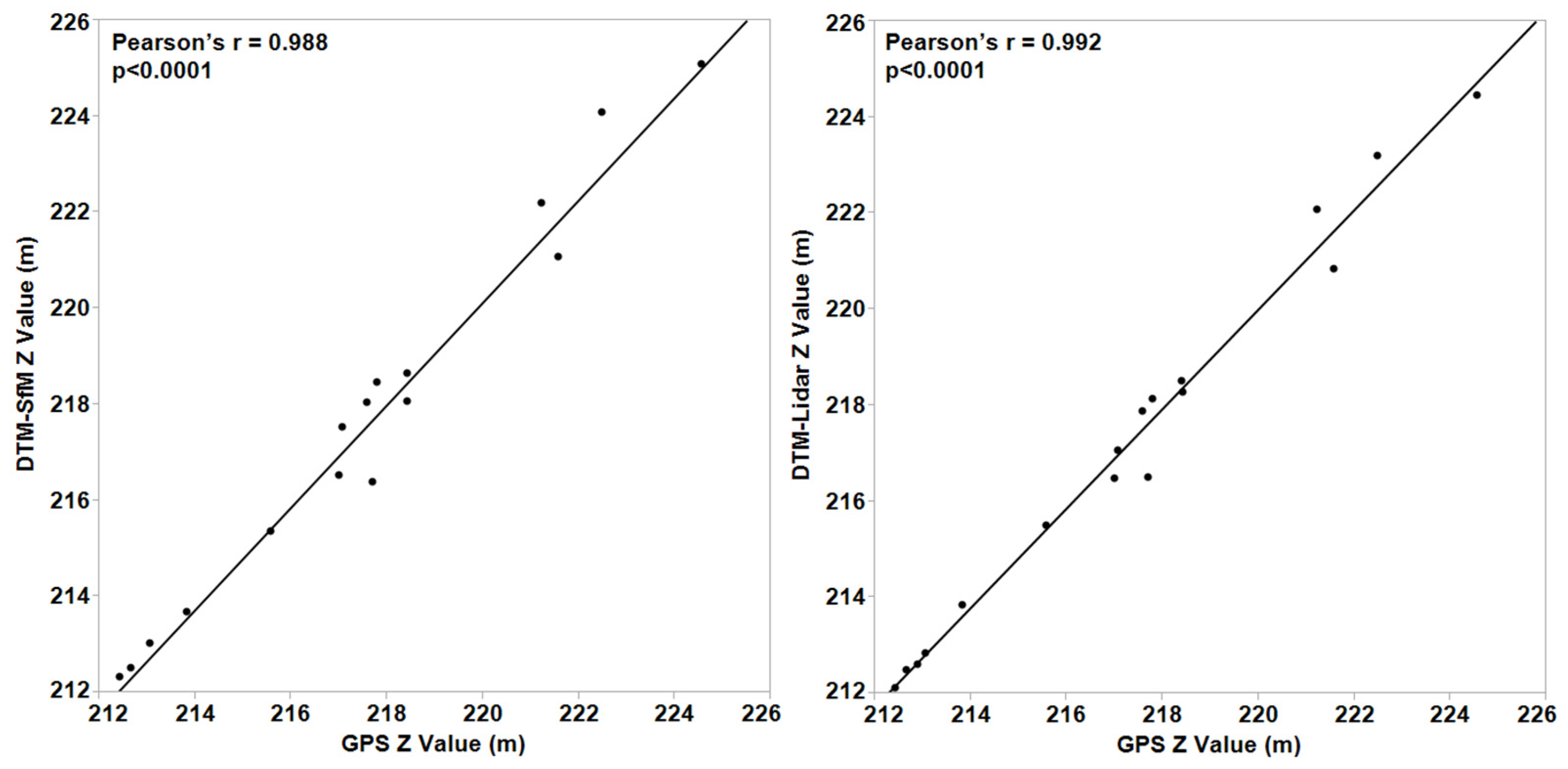
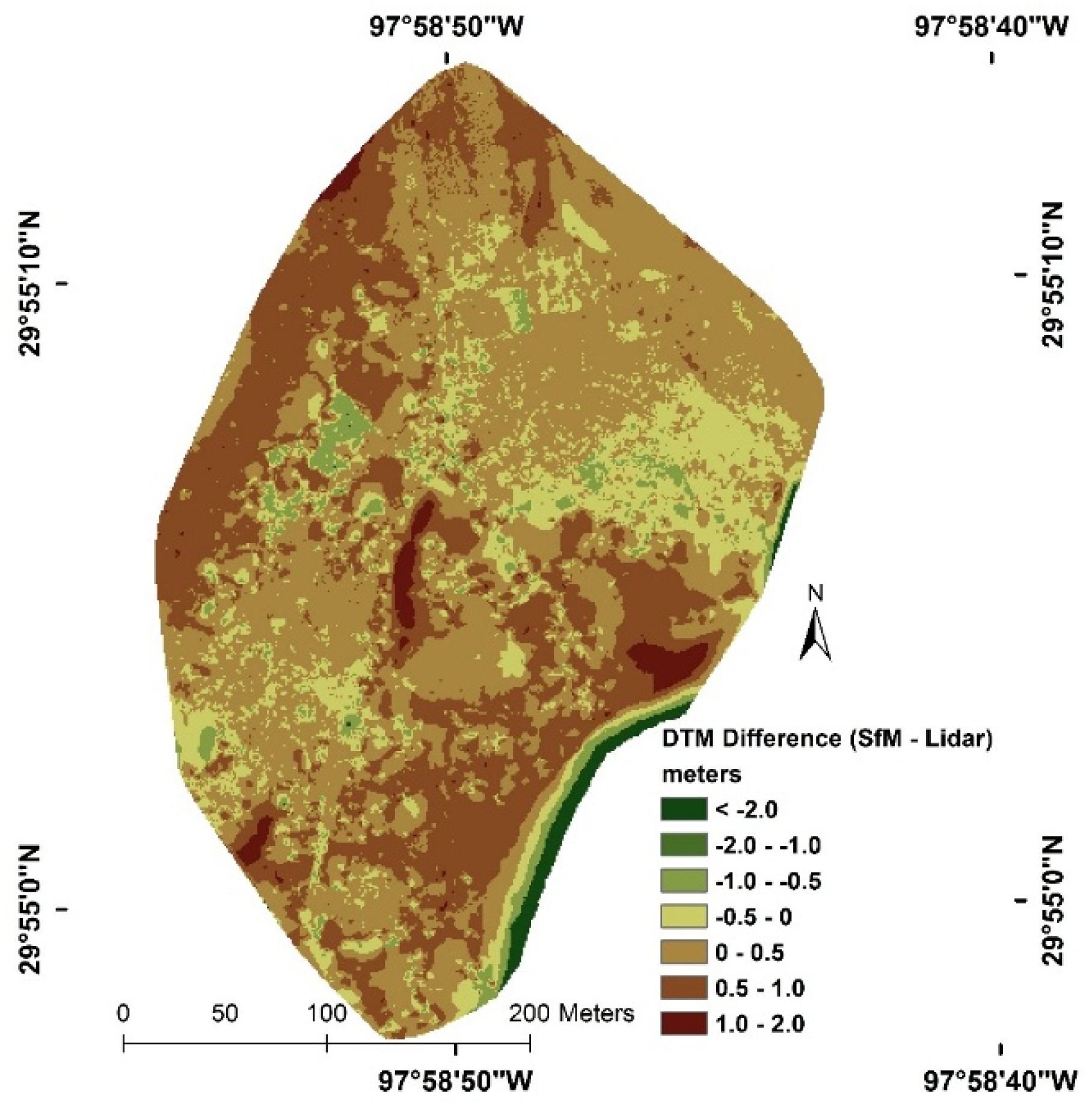
3.1. SfM and Lidar DTM Comparisons Data Analysis

Of the 9,318,164 SfM points exported from PhotoScan, 1.7 percent (161,145) were classified as ground points. In comparison, the 2006 lidar dataset of the same study area had 251,221 points in total, 19.9 percent (49,967) of which were classified as ground returns. Refer to Table 1 for a summary of point cloud characteristics per dataset and Figure 2 for a comparison of the spatial distribution of ground point densities for the SfM and lidar datasets. While the lidar data had fewer overall ground returns, they were distributed throughout the study area more evenly. In contrast, classified ground points from the SfM dataset were spatially clustered in higher densities and were absent from large portions of the study area, particularly in areas of dense vegetation cover (Figure 1).
Table 1. Summary of point cloud characteristics for the SfM and lidar datasets.
Dataset CharacteristicsSfMLidar
Total points9,318,164251,221
Ground-classified points161,14549,967
Percent ground1.719.9
Nominal point density (points/sq. m)2.580.72
Nominal point spacing (m)0.581.17
Figure 2. Point cloud densities per square meter for the ground classified SfM points (left) and ground classified lidar returns (right).
Remotesensing 08 00050 g002
Direct comparison between the GPS-surveyed vegetation plot center points and the two DTM products resulted in a mean underestimate of −0.31 m for the DTMSfM, while the DTMlidar exhibited a slight overestimate of 0.08 m. The mean difference between plot centers and the DTMSfM value was −0.31 m (st. dev. = 0.73 m) and 0.08 m (st. dev. = 0.49 m) for the DTMlidar. The DTMSfM had nearly twice the amount of error for elevation underestimation as the DTMlidar. Refer to Table 2 and Figure 3 for summaries of the GPS-based comparisons for the DTM products.
Subtracting the DTMlidar from the DTMSfM provided a spatial evaluation of the differences between the two DTM products (Figure 4). Over the entire study area, the DTMSFM tends to be within ±0.5 m to ±1.0 m of the DTMlidar. Large DTMSfM underestimates (displayed in green, Figure 4), indicate the SfM surface elevation is below the lidar surface elevation. These underestimates tend to occur in relatively open areas void of over story vegetation. DTMSfM overestimates indicate the SfM surface elevation is above the modeled lidar surface elevation. These areas, displayed in brown tones, tend to occur in areas of dense canopy cover and where lack of ground points results in greater interpolation distances. Very large DTMSfM underestimates (e.g., <−2.0 m) occur in the southeastern portion of the study area. Within this densely vegetated area, very few images were acquired, few 3D points were generated, and none were classified as ground points. Overall, the lack of ground points resulted in larger interpolation distances for this area. On average, the interpolated DTMSfM surface is 0.19 m (st. dev. = 0.66 m) higher than the interpolated DTMlidar surface.
Table 2. Summary of GPS-surveyed plot center point and DTM product comparisons.
Comparison Metrics (n = 17)GPS-DTMSfMGPS-DTMlidar
Mean difference (m)−0.310.08
Standard deviation of difference (m)0.730.49
Median difference (m)0.100.08
Minimum difference (m)−1.59−0.85
Maximum difference (m)1.291.17
Figure 3. Scatterplots showing correlation (Pearson’s r) between GPS-surveyed plot center points and DTMSfM (left) and DTMlidar (right).
Remotesensing 08 00050 g003
Figure 4. Spatial distribution of elevation differences between the DTMSfM and DTMlidar. Green tones represent areas where the DTMSfM was modeled below the DTMlidar, and brown tones represent areas above the lidar surface.
Remotesensing 08 00050 g004

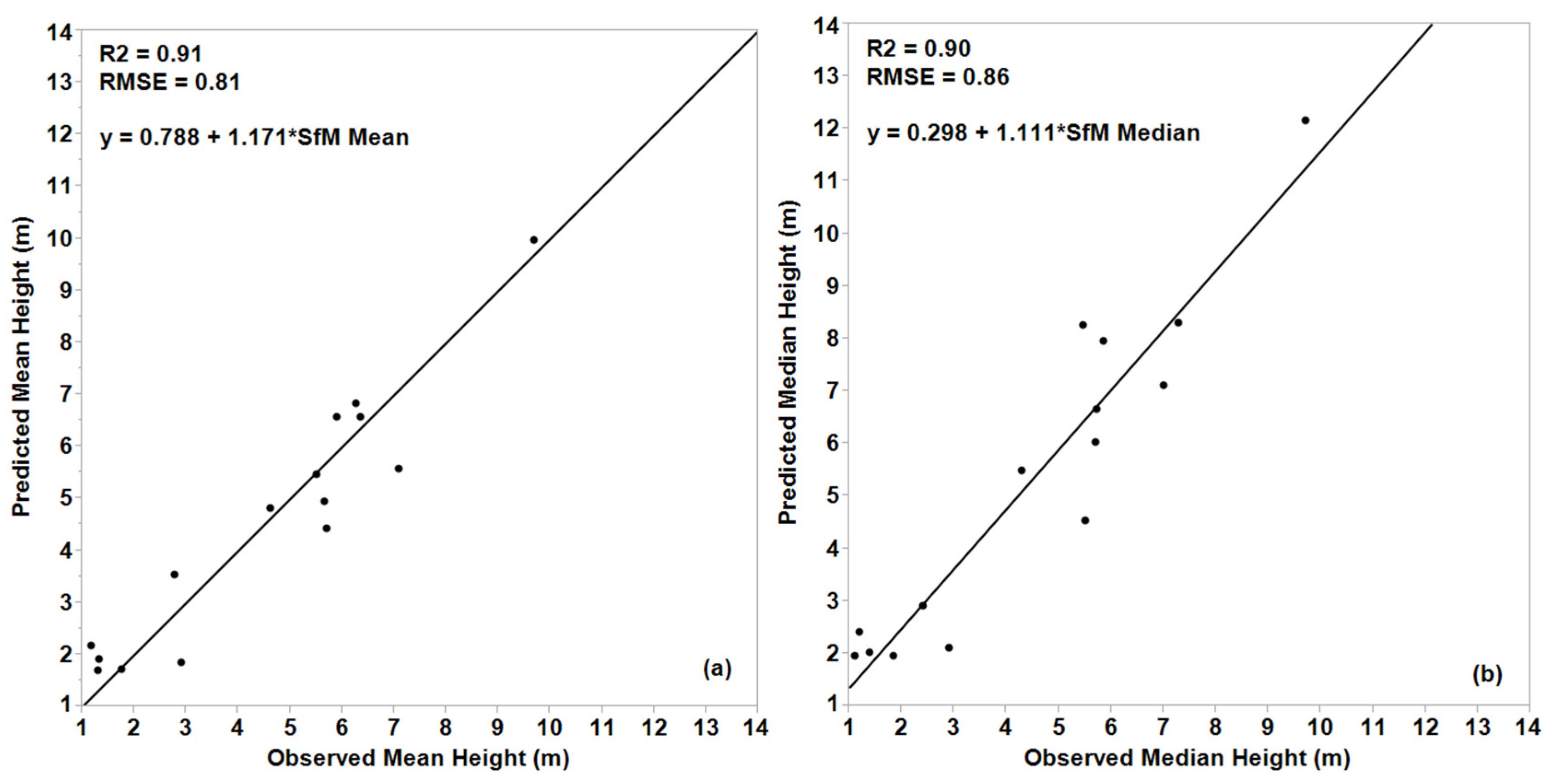
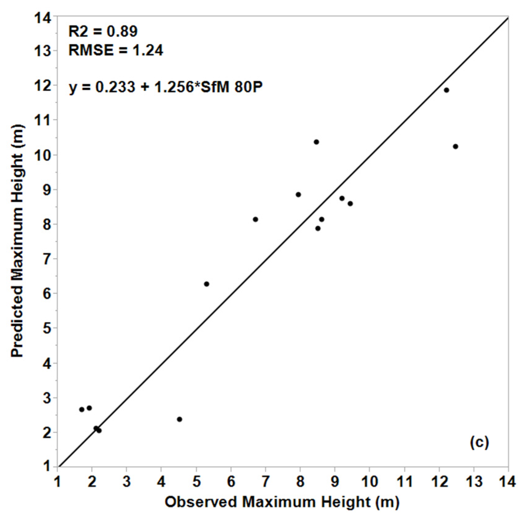
3.2. Evaluation of SfM Point Cloud Products to Estimate Tree Canopy Heights

We examined multivariate correlations between the field measured plot heights and the two sets of metrics calculated for analysis. SfMSfM refers to the use of the DTMSfM and SfM non-ground points to calculate height metrics, while SfMlidar refers to the use of DTMlidar and SfM non-ground points. In addition to multivariate correlations, we used both sets of metrics to identify simple linear regression models for three simple height measurements obtained from the field data. Fifteen field plots were included in the analysis since one of the original 16 plots had anomalously large calculated height values. We thought that manually editing the anomalous values at this point in the analysis would constitute bias, so the entire plot was excluded from the correlation and regression analyses. SfMSfM height metrics were all strongly correlated (Pearsons’s r ≥ 0.86) with field-measured plot height values with the exception of SfM maximum, which indicated a moderate correlation (Pearson’s r = 0.52–0.55) with field mean, median, and maximum plot height. Refer to Table 3 for a summary of all multivariate correlations.
Table 3. Multivariate correlations between field-measured and SfMSfM and SfMlidar plot metrics. Values represent Pearson’s r. All correlations were significant at α = 0.001. “P” refers to percentile (e.g., 95th percentile height).
Field MeanField MedField Max
SfMSfM Mean0.950.940.93
SfMSfM Med0.950.950.91
SfMSfM Max0.530.520.55
SfMSfM 95P0.880.860.91
SfMSfM 90P0.920.910.93
SfMSfM 85P0.940.920.94
SfMSfM 80P0.940.930.94
SfMlidar Mean0.940.920.95
SfMlidar Med0.950.940.93
SfMlidar Max0.470.470.51
SfMlidar 95P0.830.820.89
SfMlidar 90P0.880.890.91
SfMlidar 85P0.900.890.93
SfMlidar 80P0.900.890.93
Given the strong correlations between SfMSfM and SfMlidar height metrics and the potential for multicollinearity, we opted to perform simple linear regression to determine how well each set of metrics could predict field measured values. Models were tested by fitting individual SfMSfM or SfMlidar covariates to field measured values. In general, both SfMSfM height metrics were able to account for significant variability in field measured mean height (R2 = 0.91; RMSE = 0.81 m), median height (R2 = 0.89; RMSE = 0.91 m), and maximum height (R2 = 0.89; RMSE = 1.24 m) (Figure 5). SfMlidar height metrics performed similarly well with R2 and RMSE values nearly identical to SfMSfM-based models. Refer to Table 4 for a summary of models, their performance, and cross validation results.
Figure 5. 1:1 relationships between field-measured and model predicted mean (a) median (b) and maximum canopy height (c) and selected SfMSfM plot metrics. R2 values presented in figures represent the regression coefficient of determination. All regressions significant at p < 0.001.
Remotesensing 08 00050 g005aRemotesensing 08 00050 g005b
Table 4. Simple linear regression equations for SfMSfM and SfMlidar plot metrics and field measured plot heights. R2 value represents the regression coefficient of determination. All simple regressions were significant at p < 0.001. * symbol refers to multiplication of slope estimate and regression covariate.
SfMSfMR2 (RMSE)Kfold R2 (k = 3)SfMlidarR2 (RMSE)Kfold R2 (k = 3)
Mean Canopy Heighty = 0.788 + 1.171 * SfMSfM Mean0.91 (0.81)0.88y = 0.154 + 1.093 * SfMlidar Med0.90 (0.84)0.87
Median Canopy Heighty = 0.298 + 1.111 * SfMSfM Med0.89 (0.91)0.83y = 0.051 + 1.108 * SfMlidar Med0.89 (0.89)0.87
Max. Canopy Heighty = 0.233 + 1.256 * SfMSfM 80P0.89 (1.24)0.88y = 0.072 + 1.673 * SfMlidar Mean0.89 (1.23)0.84

4. Discussions

4.1. Image Acquisition, Processing, and Point Cloud Generation

Due to the UAS being a plane, blur within images is likely to occur due to abrupt changes in aircraft speed or attitude changes in flight. Since images with blur can negatively affect keypoint matching, they were not included, nor were any images captured at or near UAS takeoff and landing and outside of 75–125 m flying height. The reduction in images processed to generate the point cloud (i.e., 1166 originally acquired and 361 used for image matching and point cloud generation) resulted in a processing time of approximately 10 h. Moreover, although significant effort was invested to remove images with noticeable blur from image acquisition or foliage movement due to wind, some blurring in the output orthomosaic was present. It was in these areas of image blur that anomalous points were located significantly below and above the terrain surface. Although many of these values were removed prior to exporting the point cloud from PhotoScan, anomalous high (and low) Z coordinate values such as those we observed in the outlier plot removed prior to regression modeling, remained in the dataset. Such errors are typically the result of inconsistent feature matching as discussed in [22].

4.2. SfM Point Cloud Filtering and DTM Generation

A distinct advantage of lidar as a source of elevation data products is the ability to filter the dataset based on return number or order (e.g., “3 of 3 returns” or “last and only returns”). This initial filtering of a lidar dataset minimizes the number of points considered as candidate points for assignment to the ground class. SfM datasets do not possess these attributes, so quickly filtering candidate ground points can be challenging. In our study, we chose to implement a simple block minimum filter of 0.5 m to extract candidate ground points for the adaptive TIN filter provided within LP360. As with lidar datasets, a successful automatic filtering algorithm may yield a 90–95 percent accurate surface, however, the remaining 5–10 percent must be manually edited [27]. For this study, significant manual editing of ground versus non-ground points was performed due in part to the filtering algorithm used as well as the abundance of understory vegetation including grasses, shrubs, and cacti, which remained in the point cloud even after automatic filtering.
Our decision to apply a 0.5 m block filter was guided by the high point density of the dataset; 0.5 m was deemed sufficient to include points representing ground for the majority of the study area except in areas of very dense upper- and under-story canopy closure (Figure 1 and Figure 2). We emphasize that the only points used in the ground classification were points extracted from the 0.5 m block filter. In this regard, the minimum separation of ground points, and therefore interpolation distance between ground points increases as candidate points are removed from the ground class as inadvertent omission errors during the classification process. Thus, while the block minimum filter provides a large initial reduction of points, the choice of filter size influences the density of candidate ground points and ultimately the output DTM resolution. Alternate methods for initial ground point filtering and classification are available as with any traditional lidar dataset. For example, Dandois and Ellis [22] implemented a 1 m grid to extract and retain median elevation points within the point cloud and performed ground classification using a morphological filtering algorithm available in ALDPAT v1.0 [28] with good results. However, the purpose of the study was not focused on finding the optimal classification algorithm for our datasets, but instead to compare lidar and SfM products to obtain DTM surfaces and vegetation structure estimates.
The natural neighbor interpolation algorithm [29] was selected to interpolate point values to a DTM. Natural neighbor is a local adaptive operator that uses a subset of sample points surrounding a query point to interpolate heights guaranteed to be within the same range as the sample points. In the case of our study, we considered natural neighbor to be a viable interpolation algorithm since it performs well with regular and irregularly distributed data, and adapts to individual data structures without requiring sample count, search radius, or shape parameterization [30]. Although the algorithm may be considered too simplistic, prior research by Meng et al. [31] demonstrated that complex interpolation methods do not necessarily generate better results. Regardless of the technique used to identify and classify candidate ground points and the subsequent algorithm used to generate the DTM, it is clear that there are large areas in both the SfM and lidar data sets where ground points are simply not present. Our results for this specific study area demonstrate that SfM-derived point clouds can be used to generate accurate DTMs over some vegetated surfaces, though not very well in closed canopy plots or with the same semi-regular sampling distribution as the corresponding lidar dataset.

4.3. Canopy Height Estimates and Model Performance

Our results are consistent with previous studies that use image-based point clouds and derived products to estimate plot-level canopy height. However, in this case, we modeled canopy heights using DTMs generated from a classified SfM point cloud and a previously acquired lidar dataset. The simple linear regression models used to estimate mean, median, and maximum canopy height exhibited similar, and in some cases, improved coefficients of determination values and root mean square errors as reported in the lidar-based literature for a variety of vegetation cover types. Prior studies have published results demonstrating the ability of lidar-based datasets to account for approximately 70–93 percent of field measured variability with prediction errors (typically as underestimates) of roughly 1–3 m (e.g., [32,33,34,35,36]). Comparison of regression model intercepts, where the source DTM is the primary difference, indicates that when model covariates are zero, the SfMSfM models will overestimate vegetation height more so than the SfMlidar models. While these overestimates are relatively small (i.e., <1 m), accurately modeling low-lying vegetation using the SfM-derived DTM would be challenging.
Dandois and Ellis [23] used image-derived point clouds with a lidar-derived DTM to estimate mean canopy heights with moderate success (R2 = 0.64–0.74) for two study areas, though the RMSE errors were relatively high (i.e., >3.0 m). In their more recent study using a SfM-derived DTM under leaf off conditions, Dandois and Ellis [22] were able to model canopy heights of the five tallest trees per plot with improved results (R2 = 0.82–0.83), though RMSE values ranged from approximately 4 to 9 m. They note however, that the model predictions and RMSE values were similar for models that used a lidar-derived DTM. The full scope of which cover types and under what structural conditions SfM-derived point clouds can be used as an alternative to lidar data continues to be an active area of research.
The differences in model estimates and errors between metrics calculated from the DTMlidar versus the DTMSfM are minor and may be attributed to different classification algorithms, DTM resolution, etc. However, as demonstrated in this study of a 15 ha woodland, both DTM surfaces and their associated vegetation height models produced good results, though the SfM DTM did vary considerably from the lidar DTM (e.g., ±1.5 m). Exporting the low-density quality points from PhotoScan resulted in just under 200 points per square meter. Such high point density certainly facilitates characterization of some aspects of vegetation structure. However, in practice, the implementation of UAV systems to acquire imagery used to ultimately generate three dimensional point clouds over vegetated landscapes must be considered critically. Lidar is still superior in its ability to penetrate canopy gaps and record returns from the ground surface, particularly under dense canopy cover and over large areal extents.

5. Conclusions

This study presents evidence of the utility of image-based point clouds products obtained from a low-cost unmanned aerial vehicle system to provide a suitable representation of the bare earth surface under vegetation canopy as well as robust estimates (i.e., R2 ≥ 0.89) of simple plot-level canopy heights. This study is unique and significant in that our analysis provides a comparison of canopy height regression estimates derived from height metrics calculated using both a lidar-derived digital terrain model and a terrain model created from an image-based point cloud within a woodland ecosystem. We found that regardless of terrain model source data, canopy height estimates explained a substantial amount variability present in the field measured data (e.g., 89–90 percent). These results advance our knowledge of the application of image-based point clouds for natural resource modeling and monitoring by contributing information regarding the landscape conditions over which image-based point clouds can be used to both characterize the terrain surface and vegetation structure. In this regard, this study demonstrates that image-based point clouds show robust potential as a low-cost alternative source of high density three dimensional data.

Acknowledgments

We extend thanks are extended to Ethan Roberts and Caleb Jensen for their assistance with vegetation data collection and to John Klier for his assistance with image acquisition. Additionally, we also thank the three anonymous reviewers for their valuable feedback to improve the manuscript.

Author Contributions

Jennifer Jensen conceived and designed the study, participated in field data collection, analyzed the final point cloud products, performed statistical analysis and authored the paper. Adam Mathews processed and georeferenced the UAV imagery, collected field data, and co-authored the paper.

Conflicts of Interest

The authors declare no conflict of interest.

References

  1. Means, J.E.; Acker, S.A.; Fitt, B.J.; Renslow, M.; Emerson, L.; Hendrix, C.J. Predicting forest stand characteristics with airborne scanning lidar. Photogramm. Eng. Remote Sens. 2000, 66, 1367–1371. [Google Scholar]
  2. Popescu, S.C.; Wynne, R.H.; Nelson, R.F. Estimating plot-level tree heights with lidar: Local filtering with a canopy-height based variable window size. Comput. Electron. Agric. 2002, 37, 71–95. [Google Scholar] [CrossRef]
  3. Smith, A.M.S.; Falkowski, M.J.; Hudak, A.T.; Evans, J.S.; Robinson, A.P.; Steele, C.M. A cross-comparison of field, spectral, and lidar estimates of forest canopy cover. Can. J. Remote Sens. 2009, 35, 447–459. [Google Scholar] [CrossRef]
  4. Korhonen, L.; Korpela, I.; Heiskanen, J.; Maltamo, M. Airborne discrete-return lidar data in the estimation of vertical canopy cover, angular canopy closure and leaf area index. Remote Sens. Environ. 2011, 115, 1065–1080. [Google Scholar] [CrossRef]
  5. Riano, D.; Valladares, F.; Condes, S.; Chuvieco, E. Estimation of leaf area index and covered ground from airborne laser scanner (lidar) in two contrasting forests. Agric. For. Meteorol. 2004, 124, 269–275. [Google Scholar] [CrossRef]
  6. Jensen, J.L.R.; Humes, K.S.; Vierling, L.A.; Hudak, A.T. Discrete return lidar-based prediction of leaf area index in two conifer forests. Remote Sens. Environ. 2008, 112, 3947–3957. [Google Scholar] [CrossRef]
  7. Peduzzi, A.; Wynne, R.H.; Fox, T.R.; Nelson, R.F.; Thomas, V.A. Estimating leaf area index in intensively managed pine plantations using airborne laser scanner data. For. Ecol. Manag. 2012, 270, 54–65. [Google Scholar] [CrossRef]
  8. Lefsky, M.A.; Cohen, W.B.; Harding, D.J.; Parker, G.G.; Acker, S.A.; Gower, S.T. Lidar remote sensing of above-ground biomass in three biomes. Glob. Ecol. Biogeogr. 2002, 11, 393–399. [Google Scholar] [CrossRef]
  9. Hauglin, M.; Gobakken, T.; Astrup, R.; Ene, L.; Næsset, E. Estimating single-tree crown biomass of Norway spruce by airborne laser scanning: A comparison of methods with and without the use of terrestrial laser scanning to obtain the ground reference data. Forests 2014, 5, 384–403. [Google Scholar] [CrossRef]
  10. Li, W.; Niu, Z.; Huang, N.; Wang, C.; Gao, S.; Wu, C. Airborne lidar technique for estimating biomass components of maize: A case study in Zhangye City, Northwest China. Ecol. Indic. 2015, 57, 486–496. [Google Scholar] [CrossRef]
  11. Coops, N.C.; Wulder, M.A.; Culvenor, D.S.; st-Onge, B. Comparison of forest attributes extracted from fine spatial resolution multispectral and lidar data. Can. J. Remote Sens. 2004, 30, 855–866. [Google Scholar] [CrossRef]
  12. Holmgren, J. Prediction of tree height, basal area and stem volume in forest stands using airborne laser scanning. Scand. J. For. Res. 2004, 19, 543–553. [Google Scholar] [CrossRef]
  13. Ahmed, O.S.; Franklin, S.E.; Wulder, M.A. Integration of lidar and landsat data to estimate forest canopy cover in coastal British Columbia. Photogramm. Eng. Remote Sens. 2014, 80, 953–961. [Google Scholar] [CrossRef]
  14. Leberl, F.; Irschara, A.; Pock, T.; Meixner, P.; Gruber, M.; Scholz, S.; Wiechert, A. Point clouds: Lidar versus 3D vision. Photogramm. Eng. Remote Sens. 2010, 76, 1123–1134. [Google Scholar] [CrossRef]
  15. Fonstad, M.A.; Dietrich, J.T.; Courville, B.C.; Jensen, J.L.; Carbonneau, P.E. Topographic structure from motion: A new development in photogrammetric measurement. Earth Surf. Process. Landf. 2013, 38, 421–430. [Google Scholar] [CrossRef]
  16. Snavely, N. Scene Reconstruction and Visualization from Internet Photo Collections. Ph.D. Thesis, University of Washington, Seattle, WA, USA, 2008. [Google Scholar]
  17. Snavely, N.; Seitz, S.M.; Szeliski, R. Modeling the world from internet photo collections. Int. J. Comput. Vis. 2008, 80, 189–210. [Google Scholar] [CrossRef]
  18. Kaminsky, R.S.; Snavely, N.; Seitz, S.T.; Szeliski, R. Alignment of 3D point clouds to overhead images. In Proceedings of the IEEE Computer Society Conference on Computer Vision and Pattern Recognition Workshops (CVPR Workshops 2009), Miami, FL, USA, 20–25 June 2009; pp. 63–70.
  19. Mathews, A.J.; Jensen, J.L.R. Three-dimensional building modeling using structure from motion: Improving model results with telescopic pole aerial photography. In Proceedings of the 35th Applied Geography Conference, Minneapolis, MN, USA, 10–12 October 2012; Volume 35, pp. 98–107.
  20. Pollefeys, M.; Gool, L.V.; Vergauwen, M.; Verbiest, F.; Cornelis, K.; Tops, J. Visual modeling with a hand-held camera. Int. J. Comput. Vis. 2004, 59, 207–232. [Google Scholar] [CrossRef]
  21. Verhoeven, G. Taking computer vision aloft–archaeological three-dimensional reconstructions from aerial photographs with photoscan. Archaeol. Prospect. 2011, 18, 67–73. [Google Scholar] [CrossRef]
  22. Dandois, J.P.; Ellis, E.C. High spatial resolution three-dimensional mapping of vegetation spectral dynamics using computer vision. Remote Sens. Environ. 2013, 136, 259–276. [Google Scholar] [CrossRef]
  23. Dandois, J.P.; Ellis, E.C. Remote sensing of vegetation structure using computer vision. Remote Sens. 2010, 2, 1157–1176. [Google Scholar] [CrossRef]
  24. Mathews, A.; Jensen, J. Visualizing and quantifying vineyard canopy LAI using an Unmanned Aerial Vehicle (UAV) collected high density structure from motion point cloud. Remote Sens. 2013, 5, 2164–2183. [Google Scholar] [CrossRef]
  25. White, J.; Wulder, M.; Vastaranta, M.; Coops, N.; Pitt, D.; Woods, M. The utility of image-based point clouds for forest inventory: A comparison with airborne laser scanning. Forests 2013, 4, 518–536. [Google Scholar] [CrossRef]
  26. Aber, J.S.; Marzoff, I.; Ries, J.B. Small-Format Aerial Photography: Principles, Techniques and Geosciences Applications; Elsevier: Oxford, UK, 2010. [Google Scholar]
  27. Romano, M.E. Lidar processing and software. In Digital Elevation Model Technologies and Applications: The DEM Users Manual, 2nd ed.; Maune, D.F., Ed.; American Society for Photogrammetry and Remote Sensing: Bethesda, MD, USA, 2007; pp. 479–498. [Google Scholar]
  28. Zhang, K.; Cui, Z. ALDPAT 1.0. Airborne Lidar Data Processing and Analysis Tools; National Center for Airborne Laser Mapping, Florida International University: Miami, FL, USA, 2007. [Google Scholar]
  29. Sibson, R. A brief description of natural neighbor interpolation. In Interpolating Multivariate Data; Barnett, V., Ed.; John Wiley & Sons: New York, NY, USA, 1981; Volume 21, pp. 21–36. [Google Scholar]
  30. Watson, D. Contouring: A Guide to the Analysis and Display of Spatial Data; Pergamon Press: London, UK, 1992. [Google Scholar]
  31. Meng, X.; Currit, N.; Zhao, K. Ground filtering algorithms for airborne lidar data: A review of critical issues. Remote Sens. 2010, 2, 833–860. [Google Scholar] [CrossRef]
  32. Naesset, E.; Bollandsas, O.M.; Gobakken, T. Comparing regression methods in estimation of biophysical properties of forest stands from two different inventories using laser scanner data. Remote Sens. Environ. 2005, 94, 541–553. [Google Scholar] [CrossRef]
  33. Andersen, H.-E.; McGaughey, R.J.; Reutebuch, S.E. Estimating forest canopy fuel parameters using lidar data. Remote Sens. Environ. 2005, 94, 441–449. [Google Scholar] [CrossRef]
  34. Jensen, J.L.R.; Humes, K.L.; Conner, T.; Williams, C.J.; DeGroot, J. Estimation of biophysical characteristics for highly variable mixed-conifer stands using small-footprint lidar. Can. J. For. Res. 2006, 36, 1129–1138. [Google Scholar] [CrossRef]
  35. Erdody, T.L.; Moskal, L.M. Fusion of lidar and imagery for estimating forest canopy fuels. Remote Sens. Environ. 2010, 114, 725–737. [Google Scholar] [CrossRef]
  36. Saremi, H.; Kumar, L.; Turner, R.; Stone, C. Airborne lidar derived canopy height model reveals a significant difference in radiata pine (Pinus radiata D. Don) heights based on slope and aspect of sites. Trees 2014, 28, 733–744. [Google Scholar] [CrossRef]

