Comparison of Two Independent Mapping Exercises in the Primeiras and Segundas Archipelago, Mozambique

Abstract

Production of coral reef habitat maps from high spatial resolution multispectral imagery is common practice and benefits from standardized accuracy assessment methods and many informative studies on the merits of different processing algorithms. However, few studies consider the full production workflow, including factors such as operator influence, visual interpretation and a-priori knowledge. An end-user might justifiably ask: Given the same imagery and field data, how consistent would two independent production efforts be? This paper is a post-study analysis of a project in which two teams of researchers independently produced maps of six coral reef systems of the archipelago of the Primeiras and Segundas Environmental Protected Area (PSEPA), Mozambique. Both teams used the same imagery and field data, but applied different approaches—pixel based vs. object based image analysis—and used independently developed classification schemes. The results offer a unique perspective on the map production process. Both efforts resulted in similar merged classes accuracies, averaging at 63% and 64%, but the maps were distinct in terms of scale of spatial patterns, classification disparities, and in other aspects where the mapping process is reliant on visual interpretation. Despite the difficulty in aligning the classification schemes clear patterns of correspondence and discrepancy were identified. The maps were consistent with respect to geomorphological level mapping (17 out of 30 paired comparisons at more than 75% agreement), and also agreed in the extent of coral containing areas within a difference of 16% across the archipelago. However, more detailed benthic habitat level classes were inconsistent. Mapping of deep benthic cover was the most subjective result and dependent on operator visual interpretation, yet this was one of the results of highest interest for the PSEPA management since it revealed a continuity of benthos between the islands and the impression of a proto-barrier reef.

1. Introduction

Coral reef mapping from remotely sensed images is now a well-established practice, as attested by the many published papers since the early 1990s [1], books [2,3] and availability of large satellite imagery archives, and commercial image service providers. Remote sensing methods have superseded visual interpretation and manual delineation of aerial photography [4,5,6], and with the development of high spatial resolution multispectral satellite sensors (pixels < 5 m) the space data now approach the resolution of aerial photography. The digital format of satellite data facilitates computer analysis, and a variety of algorithms for producing habitat maps have been described, from basic per-pixel classification [7,8,9,10] to object based image analyses(OBIA) [11,12,13,14]. However, regardless of the mapping algorithm used, there are many aspects of map production in which operator decisions still affect the outcome: (1) choice of algorithm and parameterization; (2) choice of classification scheme; (3) visual quality checking and reprocessing; and (4) final corrections of misclassifications, i.e., contextual editing [15]. In particular, in the map production process the first analysis is rarely accepted; typically a cycle of visual assessment, adjustment and reprocessing occurs. When a map is produced for an end-user, manual correction of “obvious” misclassifications is obligatory, and the mapping process effectively becomes based on visual interpretation. While the literature contains many comparisons of different classification methods [7,8,16,17], invariably these are conducted by the same individuals or in a working-group interaction, where operator subjectivities are minimized because the aim is to assess the algorithms. However, this does not address the end-users question: generally, how reliable and consistent is map production?

The consideration of operator subjectivity in mapping quality is rarely discussed in remote sensing literature. Andréfouët [18] addresses the complexity in evaluating the human influence in the map production process, and particularly of the ones usually referred to as “experts”. One reason for the lack of information on operator subjectivity is that an analysis requires two independent mapping exercises on the same site, ideally from the same imagery and with the same field data, and this is rarely feasible. In this paper we have taken advantage of such a situation that arose from a cooperation between European Space Agency’s (ESA) G-ECO-MON project to evaluate the use of remote sensing for ecosystem services, the World Wide Fund for Nature (WWF), and Lund University, Sweden. The resulting products were two sets of benthic habitat maps for six of the islands in the Primeiras and Segundas Environmental Protected Area (PSEPA) in Mozambique: one produced by pixel based classification methodology, the other following an OBIA approach. The satellite imagery and field data were the same for both analyses and the habitat maps showed similar accuracies according to their respective methodologies in comparison to field data. However, in addition to utilizing different algorithms, the completely independent map production comprised different classification schemes, different interpretation of the field data, and different visual quality assurance processes and contextual editing. The results have not gone through any post-comparison revision. These maps are therefore an example of the possible variation from two specific providers on the same mapping task, and give an indication of both the differences and consistencies between two wholly independent production chains.

2. Study Area

The Primeiras and Segundas Environmental Protected Area (PSEPA) is located in northern Mozambique, extending over 200 km of coastline, from Pebane to Angoche. The area was declared protected in late 2012, and includes mangroves, seagrass beds and diverse coral reef habitats that support a biodiversity rich ecosystem [19]. Of the two archipelagos, distributed parallel to the coastline, only the northern, Segundas, was included in this work. The archipelago consists of seven islands, but the southern-most, Moma, was excluded from the study as field data were not collected (Figure 1).

The islands are quite small, with a maximum length of about 1 km. The smaller islands support little or no vegetation while the larger islands have some forested area. Each island is surrounded by fringing reefs in a semi-circle shape to the southeast, where massive coral colonies occur sporadically [20]. The lagoons, made of sand, coral rubble and seagrass beds, are shallow and some parts are practically exposed during low tide [20,21]. The islands have relatively exposed northern, eastern and southern sides, the latter being usually subject to monsoon influenced trade winds heading northeast during the summer or wet season (October to March) and southwest in winter or dry season (April to September) [22,23]. In general, the most developed and species diverse reefs have been reported in the most sheltered regions of the coral reef systems, i.e., facing the mainland [20]. The local waters are turbulent, not only due to upwelling but also to predominant tidal waves and irregular sea floor bathymetry, resulting in strong and quite variable currents. The main direction of the offshore surface currents is southeast, while currents at depth (100–150 meters) move towards north [23].

Figure 1. Locational map of the study area.

Figure 1. Locational map of the study area.

3. Material and Methods

3.1. Satellite Imagery Data

A mixture of 4-band WorldView2 (red, blue, green, and near-IR) and QuickBird archive imagery were used for mapping. The scenes, one per island, were selected according to the best available visibility defined by reduced extent of whitecaps and sun glint, visible deep benthic features, and generally clear waters (Table 1). Due to frequent rough seas and terrigenous plumes, clear imagery occurs infrequently, and the biggest time discrepancy between imagery and the in-situ data collection was four years. Although it is likely that the benthos has undergone some changes during this period, the structural components of the system, i.e., coral and rock, should be fairly consistent. The imagery underwent standard radiometric and sensor correction using calibration coefficients from the provider [24].

Table 1. Sensor, acquisition date and time and visibility assessment for the imagery covering each location.

	Locations	Sensor	Acquisition Date	Acquisition Time	No Whitecaps	No Sun Glint	Deep Areas Visible	Clear Waters
1	Baixo Santo Antonio	WV-2	07.12.2009	07:36:08	X		X
2	Mafamede	WV-2	18.12.2009	07:34:16			X
3	Puga Puga	QB 2	11.05.2010	07:31:05				X
4	Baixo Miguel	QB 2	11.05.2010	07:31:05				X
5	Njovo	WV-2	09.01.2010	07:32:59		X		X
6	Caldeira	WV-2	29.12.2009	07:34:14	X	X		X

Table 1. Sensor, acquisition date and time and visibility assessment for the imagery covering each location.

	Locations	Sensor	Acquisition Date	Acquisition Time	No Whitecaps	No Sun Glint	Deep Areas Visible	Clear Waters
1	Baixo Santo Antonio	WV-2	07.12.2009	07:36:08	X		X
2	Mafamede	WV-2	18.12.2009	07:34:16			X
3	Puga Puga	QB 2	11.05.2010	07:31:05				X
4	Baixo Miguel	QB 2	11.05.2010	07:31:05				X
5	Njovo	WV-2	09.01.2010	07:32:59		X		X
6	Caldeira	WV-2	29.12.2009	07:34:14	X	X		X

3.2. Benthic Cover Data

In-situ point data covering the six coral reef systems were collected by the Lund University group in two surveys, one from 15 to 17 April 2014 on the islands Mafamede, PugaPuga, Baixo Miguel and Njovo, and the second on 10 and 11 May 2014 on the islands Caldeira and Baixo Santo Antonio. The methods by which field data can be collected in this region are affected by tidal and water clarity variation as well as weather conditions. Benthic cover was observed from the boat using a clear bottom bucket: a qualitative description of the substrate and visible features were recorded, very similar to the resulting OBIA level 3 classes. Underwater photographs were taken at selected locations to illustrate different benthic cover types. Geographical coordinates were captured with a Garmin Montana 650t GPS (horizontal accuracy ± 3.65 m) [25]. Data points were taken from a slow moving boat at intervals of about 80–150 meters (as defined by the GPS receiver), but also according to observable changes of the benthic cover. Although initially planned as transects, the routes had to be adjusted to the tidal and geomorphologic characteristics of the islands for safety reasons. Data were collected by circumnavigating the reef crest, defining some transects in the lagoon and by visiting zones of interest previously defined according to the satellite imagery. The point count was intended to be approximately 200 points per island. However, due to bad weather and unsafe navigable conditions, the final dataset varied from 24 to 139 points per island, totaling about 660 geolocated points documenting benthic cover (Table 2). A more detailed description of the sampling methodology is given in Teixeira et al. [26].

Table 2. Field data distribution per location.

Location	Geolocated Points Sample Size
Baixo Santo Antonio	101
Mafamede	176
PugaPuga	103
Njovo	127
Baixo Miguel	29
Caldeira	130

Table 2. Field data distribution per location.

Location	Geolocated Points Sample Size
Baixo Santo Antonio	101
Mafamede	176
PugaPuga	103
Njovo	127
Baixo Miguel	29
Caldeira	130

3.3. Mapping Methodologies

The two map production efforts consisted of a per-pixel classification approach conducted under the G-ECO-MON project, henceforth denoted GEM, and an OBIA conducted by the Lund University group, denoted Lund. The results of both approaches included raster classification maps with per-pixel correspondence to the source images, after the conversion of the Lund polygon data. As such, the results were compared per-pixel. The classification schemes used were different, as were the methods for accuracy assessment with field data, detailed in the following sections.

3.3.1. GEM Production Effort Processing and Classification

First, the images for Njovo and Baixo Santo Antonio were corrected for water surface sun-glint using the near infra-red (NIR) band [27], while the other images were considered sufficiently free of glint that correction was not required. The purpose of the glint correction is to remove wave surface patterns that would otherwise dominate the classification, resulting in spectral reflectances values closer to how they would be if the glint was absent, and therefore more in line to those of the other images. However the correction is not perfect and residual noise may remain [28]. Images were then subject to a spatial filtering step where adjacent pixels of similar reflectance were replaced by their mean spectra, then applied iteratively until the number of distinct pixels was reduced to 10%. The spatial scale of the merging was very small (typically 3 × 3 pixels) and this step was applied to reduce single pixel scale noise in the classification. Following the recommended practice of initially classifying to at least twice the number of required classes, 60-class unsupervised k-means classification was applied. The resultant codes were ascribed to a reduced classification scheme (Table 3) by visual interpretation using historical spatially approximate Rapid Assessment documents and generalized field data. Classification was then validated using the actual contemporary geolocated field data. There were insufficient field data points to partition the data into training and validation sets, so all of the field data were reserved for accuracy assessment. Use of visual interpretation and local knowledge for training data is not only sometimes a practical necessity [29] or inherently useful [30] but it is also inevitable: no map producer would discount what they know when quality checking their classification results. Hence, operator a-priori knowledge is always relevant to map production and rarely independent from the data used for accuracy assessment. With this in mind it is important to note what background information informed the class attributions: no member of the GEM group had visited the site but several Rapid Assessment documents were available from 1997 to 2010 that described the benthic composition in roughly defined areas [21,31,32]; the in-situ data later used for accuracy assessment was also available but this was only referenced in rough geographical terms, i.e., to understand the nature of the benthic composition inside versus outside the lagoons and to define the classification scheme.

Table 3. Habitat classification scheme applied in the GEM mapping production effort.

Code	Name	Description
0	Unprocessed	No data, pixel unprocessed or invalid.
1	Land	Above water at time of image acquisition.
2	Deep water	Bottom can’t be seen in image.
3	Deep sand	Sand where bottom is only just visible, typically more than 10 m depth.
4	Shallow sand	Relatively clean sand cover, approximately less than 10 m depth, may contain some rubble and very thin vegetation.
5	Sand with thin vegetation	Sand or rubble with some seagrass and/or macroalgae cover but not sufficient to obscure the visibility of the sand substrate.
6	Dense vegetation	Dense cover of seagrass or macroalgae sufficient to obscure the substrate below.
7	Reef flat/coral and rubble field	Habitat that contains coral in a relatively sheltered environment, typically behind the reef crest and at the edge of the lagoon. Can also be spur and groove zone.
8	Reef crest/high coral cover	Places where coral is found in highest density, typically at the edge of the reef and top of the reef slope.
9	Reef slope/fore reef	High coral cover region that slopes up to the reef crest from outside the lagoon, may contain soft corals. Spur and groove formations also found here.
10	Deep benthic cover	Dark benthos barely visible in imagery, at depths 10 to 20 m, the exact nature of which cannot be determined. Could be vegetation (seagrasses or macroalgae) or deep reef structures.
11	Waves or clouds in the image	Regions where the benthos cannot be classified because breaking waves or clouds obscure it in the source image.
12	Sand on rock substrate	Corresponds to areas classed as sand in the in-situ data but they are typically raised, probably on consolidated rubble, and with thin vegetation.

Table 3. Habitat classification scheme applied in the GEM mapping production effort.

Code	Name	Description
0	Unprocessed	No data, pixel unprocessed or invalid.
1	Land	Above water at time of image acquisition.
2	Deep water	Bottom can’t be seen in image.
3	Deep sand	Sand where bottom is only just visible, typically more than 10 m depth.
4	Shallow sand	Relatively clean sand cover, approximately less than 10 m depth, may contain some rubble and very thin vegetation.
5	Sand with thin vegetation	Sand or rubble with some seagrass and/or macroalgae cover but not sufficient to obscure the visibility of the sand substrate.
6	Dense vegetation	Dense cover of seagrass or macroalgae sufficient to obscure the substrate below.
7	Reef flat/coral and rubble field	Habitat that contains coral in a relatively sheltered environment, typically behind the reef crest and at the edge of the lagoon. Can also be spur and groove zone.
8	Reef crest/high coral cover	Places where coral is found in highest density, typically at the edge of the reef and top of the reef slope.
9	Reef slope/fore reef	High coral cover region that slopes up to the reef crest from outside the lagoon, may contain soft corals. Spur and groove formations also found here.
10	Deep benthic cover	Dark benthos barely visible in imagery, at depths 10 to 20 m, the exact nature of which cannot be determined. Could be vegetation (seagrasses or macroalgae) or deep reef structures.
11	Waves or clouds in the image	Regions where the benthos cannot be classified because breaking waves or clouds obscure it in the source image.
12	Sand on rock substrate	Corresponds to areas classed as sand in the in-situ data but they are typically raised, probably on consolidated rubble, and with thin vegetation.

No depth correction or depth-invariant index calculation [33,34] was applied. Given that the sites were in large part a relatively flat shallow lagoon, with the only depth variation on the fore reef slope, it was judged that merging of the 60 classes would be adequate to handle the existence of different classes due to depth. Finally, contextual editing was used to correct misclassifications as judged by visual interpretation.

The classes used were chosen by considering the structure of the field data, and the delineations that arose naturally from unsupervised classification of the imagery. The classes were defined at habitat level and include both biotic composition and geomorphological zone. In multispectral imagery of four bands (red, green, blue, and near infra-red), only two or three convey subsurface information, so it is generally not possible to differentiate between seagrass and macroalgae by spectral reflectance alone; in fact, the field data indicated that seagrass and macroalgae often occurred together. Therefore the classification scheme included classes based on general “vegetation” which could be either seagrass or macroalgae. Typically a-priori contextual knowledge by users is required to identify areas which are dominated by seagrass. Most habitats were on a continuum where classes “sand”, “sand with thin vegetation” and “dense vegetation” were not precisely definable in terms of percentage cover but arose due to spectral gradation of image pixels. No specific level of coral cover is implied in the classes “reef slope”, “reef crest” and “reef flat”, but these can be considered places where live coral would be found.

3.3.2. GEM Production Effort Accuracy Assessment

Due to the difficultly in clearly delineating classes where mixed assemblages are common (both in the imagery classification and in-situ data) accuracy assessment was conducted by merging classes to three basic cover types: dominated by coral, sand and vegetation (seagrass or algae). This was also necessary because the in-situ data contained only small number of instances of some classes, and even with this merging, the “vegetation” class was absent in the in-situ data at three of the six islands. Confusion matrices for these three classes (and including “deep water” for the map data) were constructed for the six islands.

3.3.3. Lund Production Effort Processing and Classification

The first pre-processing step applied in the OBIA was to maximize the visual contrast of the images by a combination of radiometric correction, principal component analysis, dark object subtraction, sun glint correction according to Hedley et al. [27] and water column correction according to Lyzenga [33,34].

The imagery was iteratively segmented and classified according to a three level hierarchical classification scheme based on shallow water coral reef environment research work by Mumby and Harborne [35], Rohmann [36] and Andréfouët [37]. The classification scheme (Table 4) was adapted to the field data and imagery so as to maximize the variety of benthic habitats included. Segmentation was performed using Trimble eCognition Developer’s multiresolution segmentation algorithm, applying a decreasing scale parameter (100 to 5), while compactness and color were kept almost constant (0.7 to 0.9). Due to the variation within the images, the parameters were adjusted to the individual datasets. Classification was performed using the Nearest Neighbor classification algorithm, including Feature Optimization tools. Training datasets were created by the operator based on image interpretation informed by the field data, together with empirical knowledge of the coral reef systems. The Lund team had physically visited the site and collected the in-situ data, but in attempt to promote independence from the in-situ data sets, the training sites were selected from areas not covered by the field data.

Maps were created for each level of the hierarchical classification, resulting in three maps per reef system. Finally, contextual editing was applied to correct misclassifications according to visual interpretation. Further information on the image processing can be found in Teixeira et al. [26].

3.3.4. Lund Production Effort Accuracy Assessment

Confusion matrices were generated for the resulting bottom cover and benthic habitat maps (levels 2 and 3) using the field data points. All classes present in the map were included in the accuracy assessment, despite insufficient distribution of point data across classes.

Table 4. Three level hierarchical habitat classification scheme applied in the Lund mapping production effort.

Level 1	Level 2	Level 3
Geomorphological Zone	Bottom Cover	Benthic Habitat
Land	Land	Land
Shallow waters	Sand	Sand
Lagoon/Reef crest/Fore reef	Sand/Rubble	Sand/Rubble
		with Seagrass
		with Seagrass and Rocks
		with Seagrass and Rocks with Brown Macroalgae
		with Rocks
		with Rocks with Brown Macroalgae
	Rock	Rock
		with Brown Macroalgae
		with Sand and Rubble
		with Brown Macroalgae and Sand and Rubble
	Coral	Coral
		Spur and Groove
		Field
		Patches
Deep (fore) reef	Sand	Sand
	Deep benthic cover	Deep benthic cover
Deep water	Deep water	Deep water
No information	No information	No information

Table 4. Three level hierarchical habitat classification scheme applied in the Lund mapping production effort.

Level 1	Level 2	Level 3
Geomorphological Zone	Bottom Cover	Benthic Habitat
Land	Land	Land
Shallow waters	Sand	Sand
Lagoon/Reef crest/Fore reef	Sand/Rubble	Sand/Rubble
		with Seagrass
		with Seagrass and Rocks
		with Seagrass and Rocks with Brown Macroalgae
		with Rocks
		with Rocks with Brown Macroalgae
	Rock	Rock
		with Brown Macroalgae
		with Sand and Rubble
		with Brown Macroalgae and Sand and Rubble
	Coral	Coral
		Spur and Groove
		Field
		Patches
Deep (fore) reef	Sand	Sand
	Deep benthic cover	Deep benthic cover
Deep water	Deep water	Deep water
No information	No information	No information

3.4. Mapping Results Comparison

Since there was no previous intention of conducting a comparative study, the classification schemes were developed independently, which led to relatively few classes having a direct 1:1 correspondence between the two map production efforts and class grouping being required (Table 5). For geomorphological categories, level 1 in the Lund maps, identifying corresponding classes or groupings was fairly straightforward for “Land”, “Shallow surround” (shallow areas outside the fore reef), “Reef crest”, “Fore reef” and “Deep water”. Likewise, the bottom cover (level 2) maps were used in the assessment of “Deep benthic cover” (dark benthos of unknown composition in deep water), “Coral containing” areas (places where live coral would be found), and three different comparisons for bare sand or rock, “Bare 1–3”. The benthic habitat classes at level 3 were considered too specific to provide a relevant assessment of direct map correspondence. Therefore, it was not possible to compare mixed classes with vegetated cover directly, so all classes that included seagrass and/or brown macroalgae were aggregated and compared to the GEM class “Dense vegetation”. A comparison between GEM “Dense vegetation” and Lund “Sand” was also included because it was apparent from visual interpretation that this could have a high correspondence.

The maps from the two production efforts were initially compared by visual assessment, supported by the calculation of the edge similarity index for the pairs of classes referring to coral, vegetation and deep benthic cover. This index, ranging from 0 to 1, represents the percentage of overlap of class boundaries, thus assessing geometric correspondence between the maps products. As recommended by Lizarazo [38], the edges were considered as overlapping within a tolerance zone, here defined as a buffer of approximately two times the sensor ground resolution, i.e., a total of four meters for WV-2 and five meters for QB 2 images.

Table 5. Pairing of selected classes for comparisons.

Comparison	GEM Classes	Lund Classes	OBIA Level
Geomorphology level
Land	Land	Land	1
Shallow surround	Shallow sand	Shallow waters	1
Reef crest	Reef crest/high coral cover	Reef crest	1
Fore reef	Reef slope/fore reef	Fore reef	1
Deep water	Deep water	Deep water	1
Benthic habitat level
Deep benthic cover	Deep benthic cover	Deep benthic cover	2
Bare 1	Sand with thin vegetation	Sand	2
Bare 2	Sand over rock substrate	Sand	2
Bare 3	Sand over rock substrate	Rock	2
Vegetation-sand confusion	Dense vegetation	Sand	2
Vegetation	Dense vegetation	Sand/Rubble with Seagrass	3
		Sand/Rubble with Seagrass and Rocks
		Sand/Rubble with Seagrass and Rocks with Brown Macroalgae
		Sand/Rubble with Rocks with Brown Macroalgae
		Rock with Brown Macroalgae, and
		Rock with Brown Macroalgae and Sand and Rubble
Coral containing	Reef crest/high coral cover and Reef slope/fore reef	Coral	2

Table 5. Pairing of selected classes for comparisons.

Comparison	GEM Classes	Lund Classes	OBIA Level
Geomorphology level
Land	Land	Land	1
Shallow surround	Shallow sand	Shallow waters	1
Reef crest	Reef crest/high coral cover	Reef crest	1
Fore reef	Reef slope/fore reef	Fore reef	1
Deep water	Deep water	Deep water	1
Benthic habitat level
Deep benthic cover	Deep benthic cover	Deep benthic cover	2
Bare 1	Sand with thin vegetation	Sand	2
Bare 2	Sand over rock substrate	Sand	2
Bare 3	Sand over rock substrate	Rock	2
Vegetation-sand confusion	Dense vegetation	Sand	2
Vegetation	Dense vegetation	Sand/Rubble with Seagrass	3
		Sand/Rubble with Seagrass and Rocks
		Sand/Rubble with Seagrass and Rocks with Brown Macroalgae
		Sand/Rubble with Rocks with Brown Macroalgae
		Rock with Brown Macroalgae, and
		Rock with Brown Macroalgae and Sand and Rubble
Coral containing	Reef crest/high coral cover and Reef slope/fore reef	Coral	2

Additionally, each island’s map was overlaid to develop confusion matrices of class correspondence between the GEM and Lund products. This led to a total of 18 confusion matrices quantifying the spatial agreement of the selected classes. To understand the consistency of the mapping results across the six islands, Wilcoxon Signed-Ranks test and linear intercorrelation were applied to the number of pixels coinciding for each selected class pair. Wilcoxon’s p-value for paired samples indicates the probability that the observed results would happen if the null hypothesis were true, i.e., if the median of the differences of the samples were zero. Thus, small values of p-value show that there is a systematic over- or underestimation over the six islands, whereas a non-significant result means either the agreement was very good between the two production methods or the production methods disagreed but in a non-systematic way. The coefficient of determination of the linear intercorrelation provides an evaluation of how much the quantification resulting from one methodology is reliable as a predictor for the quantification of the other. In both production efforts each island was mapped independently, so evaluating the results across the six islands will reveal any systematic biases in the production methods, encompassing both mapping algorithm and operator dependent factors.

The applicability of the maps as natural resources management tools was assessed by evaluating the consistency of the maps in answering hypothetical questions based on information needs from the PSEPA’s management:

(1)

What is the extent of coral containing habitats per island, and the total within the protected area?

(2)

What is the extent of macroalgae or seagrass areas per island, and the total within the protected area?

(3)

Where are areas of deep benthic cover to be found, possibly currently unknown and a future focus for field surveys?

The values of the extents of coral, vegetation and deep benthic cover were estimated according to the class groups already presented, although this grouping could be different depending on the interpretation of the end user, particularly for the study of vegetation.

4. Results and Discussion

4.1. Accuracy Assessment, Edge Similarity and Class Agreement Results

Accuracy assessment with respect to the field data indicated the maps have variable but generally reasonable accuracy: 56% to 72% for GEM and 43% to 93% for Lund (Table 6). These values are considered adequate for management and planning purposes, for which a value of about 60% is generally recommended [3,39]. Moreover, the obtained results fall within the range of values found in current research results of coral reef habitat mapping [7,12,18,40]. Therefore, both production efforts resulted in maps that were generally of a defensible quality in a benthic habitat mapping context.

Table 6. Accuracy assessment results for the pixel based and object based maps.

Island	GEM	Lund
	Generalized Three Class Product (%)	Level 2 (%)	Level 3 (%)
Baixo Santo Antonio	58	91	74
Mafamede	66	93	56
Puga Puga	63	83	60
Baixo Miguel	72	44	35
Njovo	61	82	55
Caldeira	56	58	43

Table 6. Accuracy assessment results for the pixel based and object based maps.

Island	GEM	Lund
	Generalized Three Class Product (%)	Level 2 (%)	Level 3 (%)
Baixo Santo Antonio	58	91	74
Mafamede	66	93	56
Puga Puga	63	83	60
Baixo Miguel	72	44	35
Njovo	61	82	55
Caldeira	56	58	43

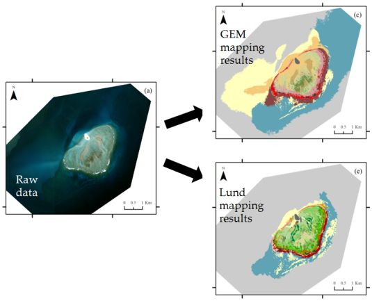
A first, rough visual assessment of the mapping outputs (Figure 2), conducted by overlapping the three OBIA maps on the pixel based ones, allowed the identification of clear differences. While land and the overall shape of the coral reef system matched well, the deep benthic classes—deep benthic cover and deep sand—were often more extensive in GEM maps. Another observation is that the benthic habitat (level 3) Lund maps show more clearly delineated areas, particularly within the lagoon and reef crest, while avoiding the “salt and pepper” effect, which is a frequently identified advantage of the object based approach [14,41,42].

The edge similarity results support the visual interpretation, quantifying the deep benthic cover edge correspondence as ranging from 2% to 16% (Table 7). The remaining class comparisons, more complex to assess visually due to the number of classes included, shows a general good level of agreement, with an edge similarity index in order of 10% to 30% for coral containing classes and above 30% for vegetation in the majority of the locations.

The confusion matrices comparing the map pairs show very high (>75%) class agreement for “Land”, “Fore reef” and “Deep water” in all the six study locations (Table 8). Two of the comparisons related to sand or rock substrate, “Bare 1” and “Bare 2”, had a very high agreement for about half of the locations, while “Bare 3” (Sand over rock substrate vs. Rock) had very high agreement only at one. The “Coral containing” comparison had very good agreement at three sites and poor agreement at only one. Additionally, from the 18 generated confusion matrices, it was possible to observe that “Sand on rock substrate”, “Dense vegetation” and “Sand with thin vegetation” display a high level of agreement with the class “Lagoon” from the Lund classification scheme. This result was expected, and supports adequate spatial correspondence of classes, as these three are generally found in that geomorphological zone.

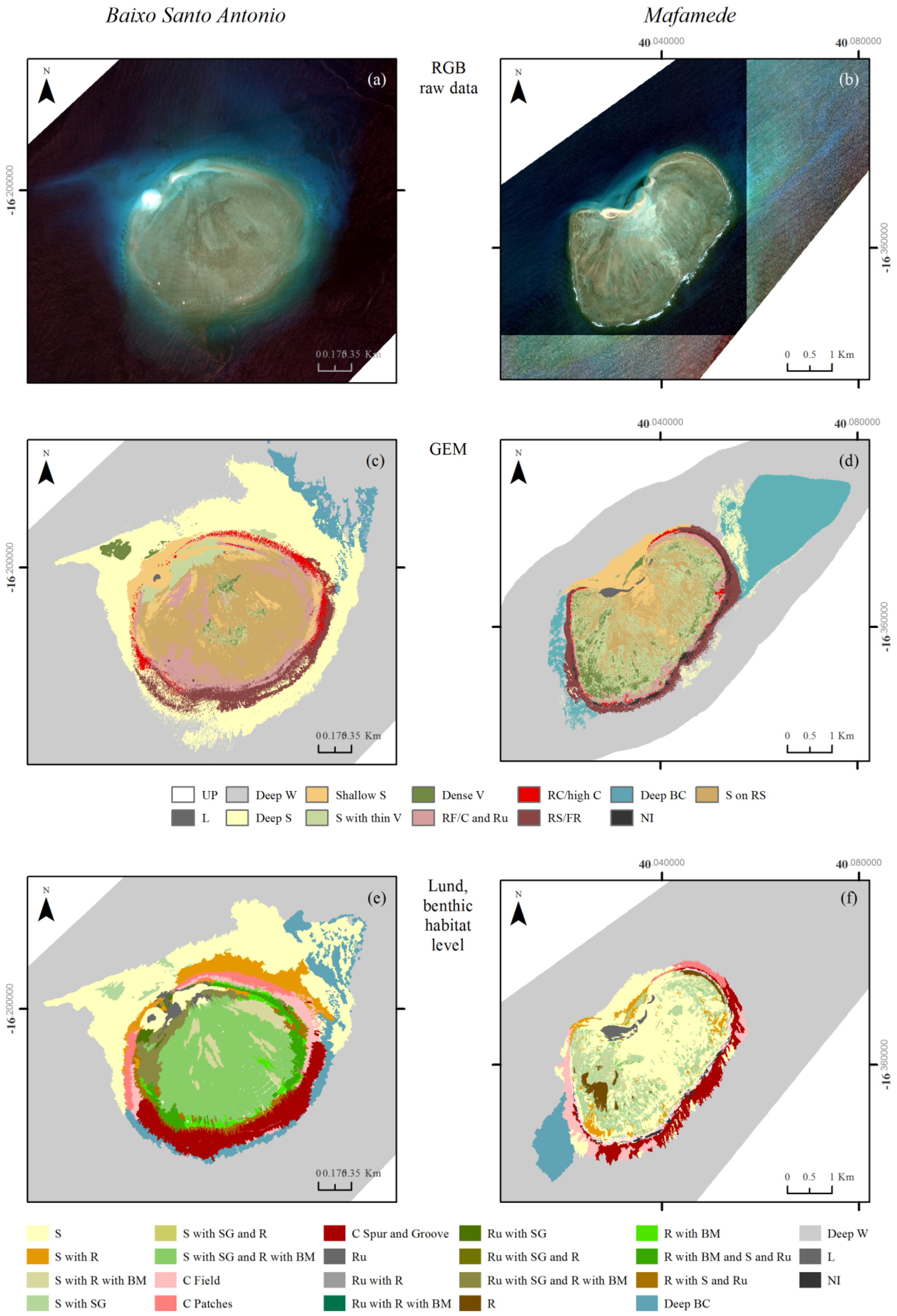
Figure 2. Example of (a,b) raw data (min and max percentage clip = 0.2); (c,d) GEM and (e,f) Lund mapping results for Baixo Santo Antonio and Mafamede; BC=benthic cover, BM = brown macroalgae, C = coral, FR = fore reef, L = land, NI = No information, R=rock(s), RC = reef crest, RF = reef front, RS = reef slope, Ru = rubble, S = sand, SG = seagrass, UP=unprocessed,V = vegetation, W = water.

Figure 2. Example of (a,b) raw data (min and max percentage clip = 0.2); (c,d) GEM and (e,f) Lund mapping results for Baixo Santo Antonio and Mafamede; BC=benthic cover, BM = brown macroalgae, C = coral, FR = fore reef, L = land, NI = No information, R=rock(s), RC = reef crest, RF = reef front, RS = reef slope, Ru = rubble, S = sand, SG = seagrass, UP=unprocessed,V = vegetation, W = water.

Table 7. Edge similarity index values for results for selected pairs of classes.

Island	Coral (%)	Vegetation (%)	Deep Benthic Cover (%)
Baixo Santo Antonio	12.3	6.5	16.3
Mafamede	39.7	77.6	1.6
PugaPuga	8.9	33.4	6.8
Baixo Miguel	7.3	20.3	4.2
Njovo	35.9	58.6	12.8
Caldeira	32.1	45.5	2.3

Table 7. Edge similarity index values for results for selected pairs of classes.

Island	Coral (%)	Vegetation (%)	Deep Benthic Cover (%)
Baixo Santo Antonio	12.3	6.5	16.3
Mafamede	39.7	77.6	1.6
PugaPuga	8.9	33.4	6.8
Baixo Miguel	7.3	20.3	4.2
Njovo	35.9	58.6	12.8
Caldeira	32.1	45.5	2.3

The class comparison “Shallow surround”, “Bare 2” and “Deep benthic cover” show a very low agreement (<50%) for the majority of the locations.

Table 8. Class agreement matrix results for selected pairs of classes.

Comparison	Baixo Santo Antonio	Mafamede	PugaPuga	Baixo Miguel	Njovo	Caldeira
Land	100.0	99.8	99.9	-	99.8	99.5
Shallow surround	46.4	28.8	24.9	71.7	18.0	16.7
Reef crest	2.1	35.3	14.1	7.5	33.3	49.6
Fore reef	80.4	79.0	80.4	80.4	80.4	80.4
Deep benthic cover	34.9	1.5	25.0	51.1	2.7	8.2
Deep water	98.5	92.2	99.9	95.2	97.9	99.4
Bare 1	57.7	94.1	77.8	35.5	79.9	37.0
Bare 2	80.0	95.3	62.9	31.4	51.1	65.6
Bare 3	11.2	3.4	9.8	58.5	48.7	10.2
Vegetation-sand confusion	96.2	96.1	77.9	35.6	63.0	56.8
Vegetation	82.1	65.9	36.8	89.3	68.1	90.8
Coral containing	81.7	79.6	35.0	57.5	61.2	85.7

Table 8. Class agreement matrix results for selected pairs of classes.

Comparison	Baixo Santo Antonio	Mafamede	PugaPuga	Baixo Miguel	Njovo	Caldeira
Land	100.0	99.8	99.9	-	99.8	99.5
Shallow surround	46.4	28.8	24.9	71.7	18.0	16.7
Reef crest	2.1	35.3	14.1	7.5	33.3	49.6
Fore reef	80.4	79.0	80.4	80.4	80.4	80.4
Deep benthic cover	34.9	1.5	25.0	51.1	2.7	8.2
Deep water	98.5	92.2	99.9	95.2	97.9	99.4
Bare 1	57.7	94.1	77.8	35.5	79.9	37.0
Bare 2	80.0	95.3	62.9	31.4	51.1	65.6
Bare 3	11.2	3.4	9.8	58.5	48.7	10.2
Vegetation-sand confusion	96.2	96.1	77.9	35.6	63.0	56.8
Vegetation	82.1	65.9	36.8	89.3	68.1	90.8
Coral containing	81.7	79.6	35.0	57.5	61.2	85.7

The GEM classes “Deep sand” and “Deep benthic cover” mostly coincided with the Lund class “No information”, which represents locations where it was considered the sea bottom was not visible, which included not only deep water but also cloud cover, white caps and sun glint. As the number of pixels with the above-surface features is much smaller than those over deep water, “No information” was used as a direct equivalent of “Deep water”. These results support the visual interpretation of the maps, where the majority of the deep feature identified in the pixel based maps corresponds to deep water in the object based maps. Identifying the deepest bottom features by visual interpretation requires using various stretches of the imagery to infer where features are and so is to some extent subjective, being reliant on the effort put by the operator into it. Nevertheless, the human eye remains more powerful than automated analysis for identifying subtle and noisy spatial patterns so visual interpretation is a valuable tool in deep areas, even if it does not comprise of a systematic analysis. In particular, the fundamental limitation in deep waters is that relatively few photons that reach the sensor have interacted with the bottom, and no processing algorithm can compensate for this [43]. The greater extent of the “Deep sand” and “Deep benthic cover” classes in the pixel based production (Figure 2c–f, Figure 3c–f and Figure 4c–f) is probably in large part due to the effort and interpretation of the operator.

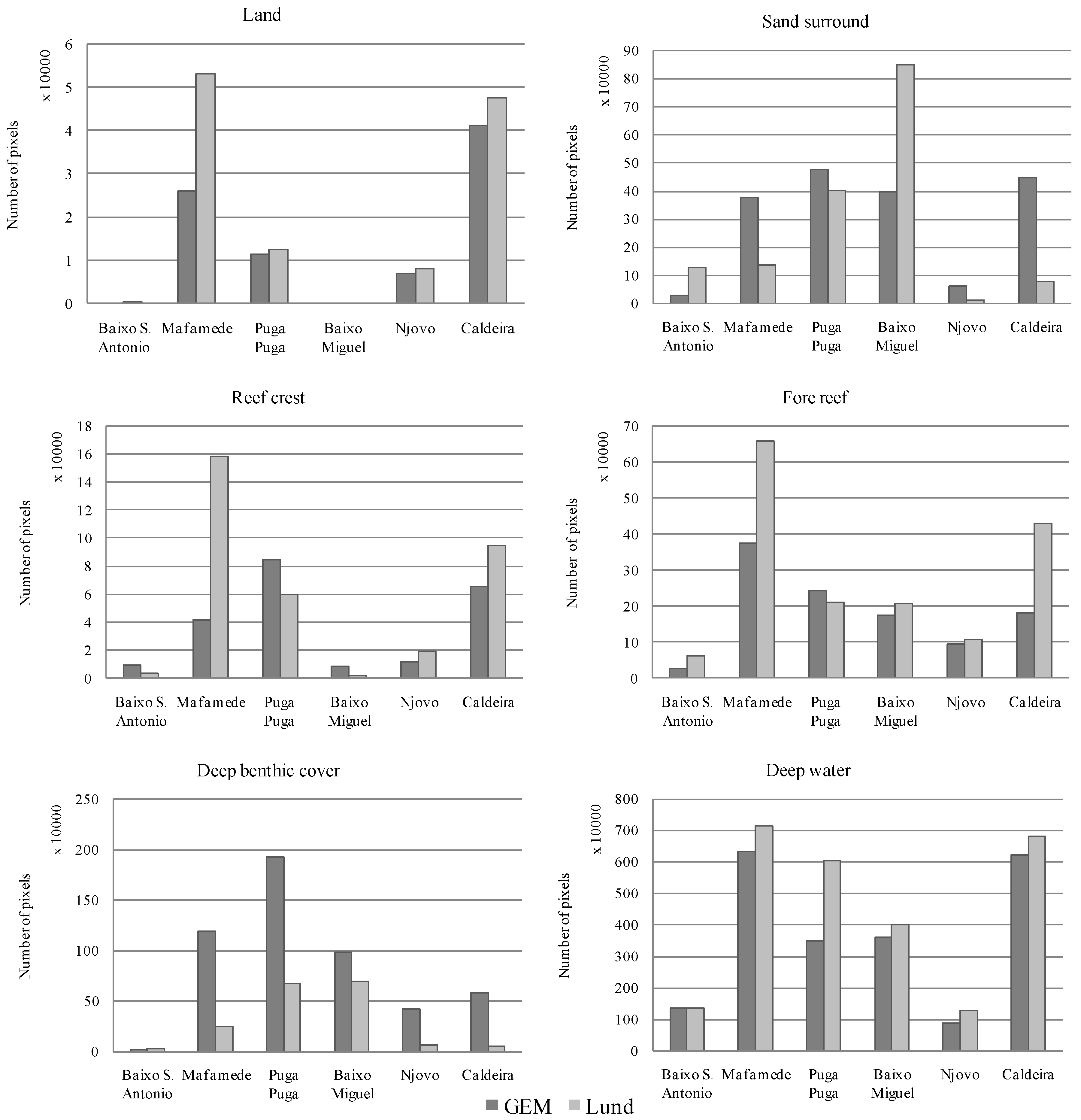
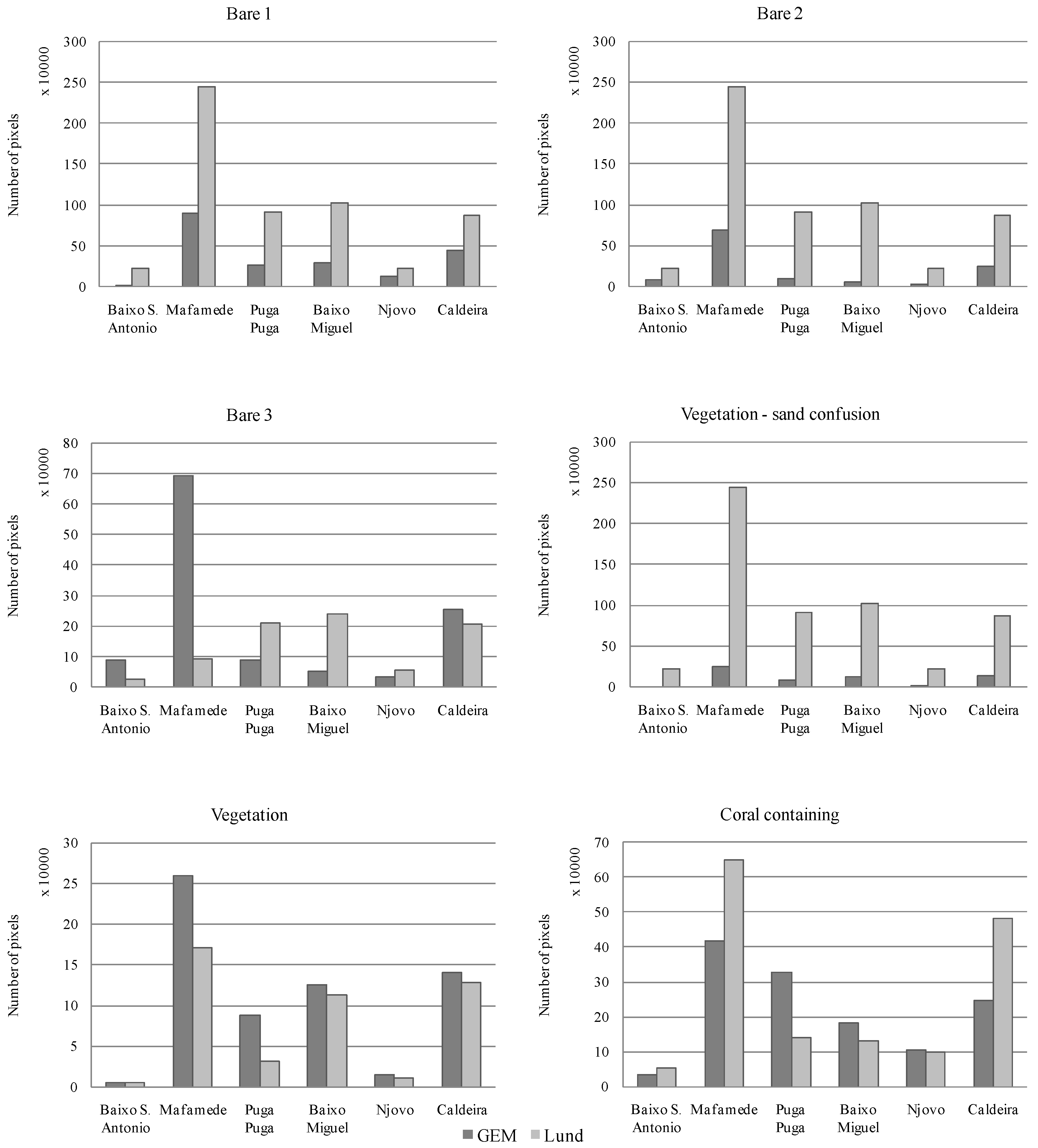
When comparing the number of pixels mapped for the selected class pairs, it is clear that results are in general similar for class pairs at the geomorphological level (Figure 5), but less so at the benthic habitat level (Figure 6). However, there is good agreement for the comparison of Coral containing areas and Vegetation.

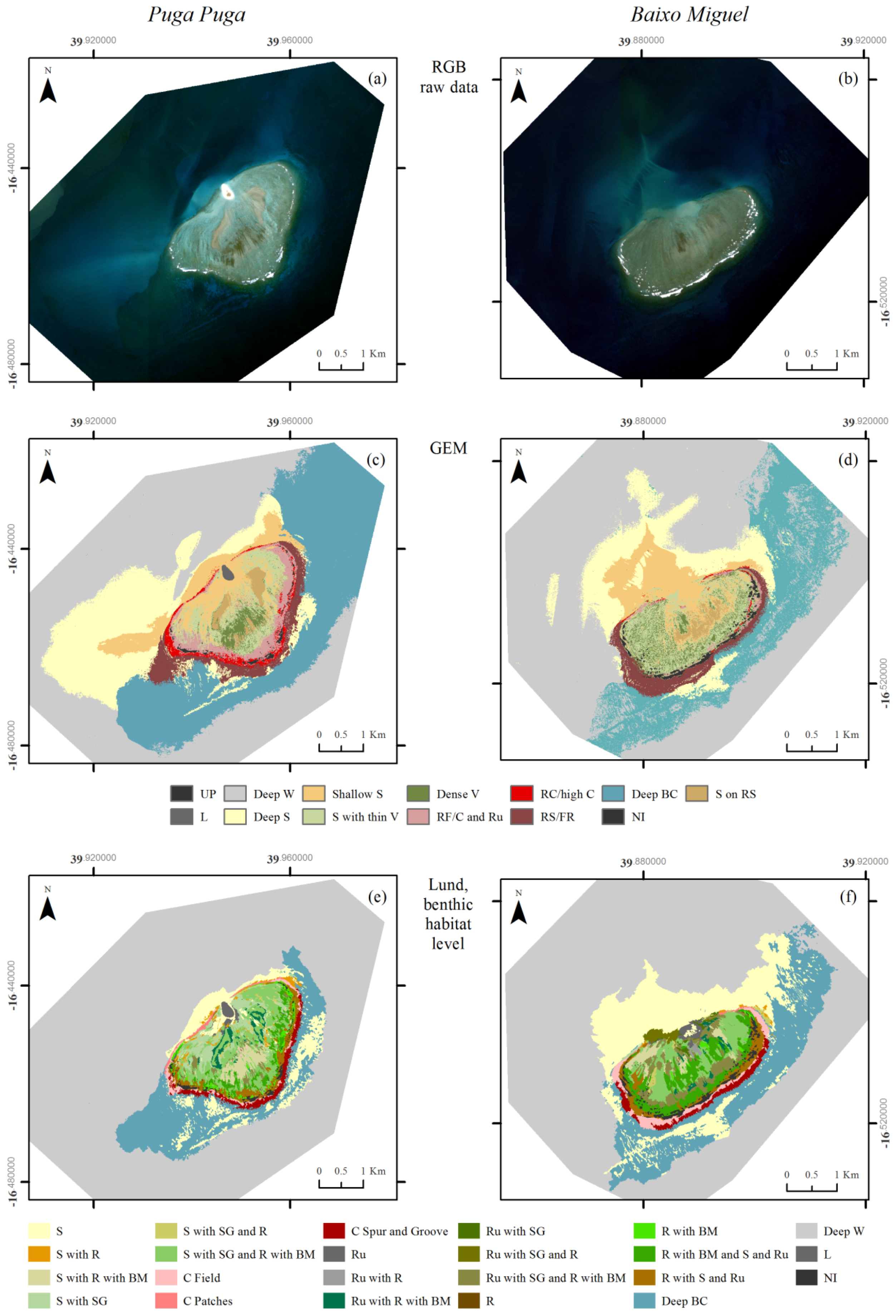
Figure 3. Example of (a,b) raw data (min and max percentage clip = 0.2); (c,d) GEM and (e,f) Lund mapping results for PugaPuga and Baixo Miguel; BC = benthic cover, BM = brown macroalgae, C = coral, FR = fore reef, L = land, NI = No information, R = rock(s), RC = reef crest, RF = reef front, RS = reef slope, Ru = rubble, S = sand, SG = seagrass, UP=unprocessed,V = vegetation, W = water.

Figure 3. Example of (a,b) raw data (min and max percentage clip = 0.2); (c,d) GEM and (e,f) Lund mapping results for PugaPuga and Baixo Miguel; BC = benthic cover, BM = brown macroalgae, C = coral, FR = fore reef, L = land, NI = No information, R = rock(s), RC = reef crest, RF = reef front, RS = reef slope, Ru = rubble, S = sand, SG = seagrass, UP=unprocessed,V = vegetation, W = water.

Figure 4. Example of (a,b) raw data (min and max percentage clip = 0.2); (c,d) GEM and (e,f) Lund mapping results for Njovo and Caldeira; BC = benthic cover, BM = brown macroalgae, C = coral, FR = fore reef, L = land, NI = No information, R = rock(s), RC = reef crest, RF = reef front, RS = reef slope, Ru = rubble, S = sand, SG = seagrass, UP=unprocessed,V = vegetation, W = water.

Figure 4. Example of (a,b) raw data (min and max percentage clip = 0.2); (c,d) GEM and (e,f) Lund mapping results for Njovo and Caldeira; BC = benthic cover, BM = brown macroalgae, C = coral, FR = fore reef, L = land, NI = No information, R = rock(s), RC = reef crest, RF = reef front, RS = reef slope, Ru = rubble, S = sand, SG = seagrass, UP=unprocessed,V = vegetation, W = water.

Figure 5. Paired class comparison across the different coral reef systems at the geomorphological level; GEM refers to the pixel based mapping products, and Lund to the OBIA mapping.

Figure 5. Paired class comparison across the different coral reef systems at the geomorphological level; GEM refers to the pixel based mapping products, and Lund to the OBIA mapping.

4.2. Systematic Biases in Production Methods

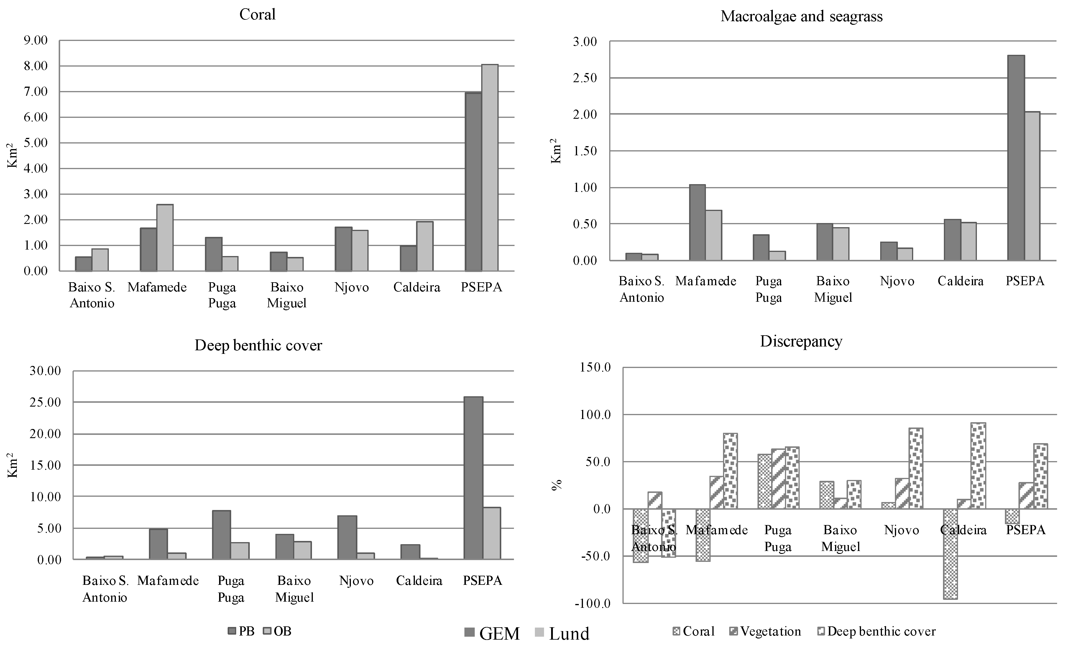
The results show low p-values (<0.001) for half of the classes, confirming that there is indeed systematic over- or underestimation of the mapped classes (Table 9), but this could arise simply from the fact that the class groupings do not quite represent the same things in the two analyses. However the comparisons for “Shallow surround”, “Reef crest”, “Fore reef”, “Deep benthic cover”, “Bare 3” and “Coral containing” do not exhibit statistically significant systematic over- or underestimation (i.e., p > 0.05).

Figure 6. Paired class comparison across the different coral reef systems at the bottom cover and benthic habitat levels.

Figure 6. Paired class comparison across the different coral reef systems at the bottom cover and benthic habitat levels.

This result is not surprising, as most of the class groupings don’t correspond exactly to each other, due to the similarity in the islands configuration and composition, systematic over- or underestimation might be expected, rather than a combination of both. It is interesting to notice that the classes likely to represent the same extent refer to features with either very clear spectral signal (such as shallow sand), easy to identify visually (such as reef crest), or fairly stable features (such as geomorphological structures and coral), although their correlation was low. On the other hand, the classes that indicated under- and/or overestimation obtained a high level of agreement, likely due to the quite often larger extent of the object based results for the selected pairs (Figure 5).

Table 9. Wilcoxon signed-rank test for paired samples results (p-value, W) and linear intercorrelation strength (r²).

Comparison	p-Value	W	r2
Land	<0.001	0	0.861
Shallow surround	>0.2	9	0.200
Reef crest	>0.2	7	0.321
Fore reef	0.05–0.10	2	0.759
Deep benthic cover	0.05–0.10	1	0.629
Deep water	<0.001	0	0.890
Bare 1	<0.001	0	0.923
Bare 2	<0.001	0	0.812
Bare 3	>0.2	10	0.012
Vegetation	<0.001	0	0.902
Vegetation-sand confusion	<0.001	0	0.931
Coral containing	>0.2	8	0.574

Table 9. Wilcoxon signed-rank test for paired samples results (p-value, W) and linear intercorrelation strength (r²).

Comparison	p-Value	W	r2
Land	<0.001	0	0.861
Shallow surround	>0.2	9	0.200
Reef crest	>0.2	7	0.321
Fore reef	0.05–0.10	2	0.759
Deep benthic cover	0.05–0.10	1	0.629
Deep water	<0.001	0	0.890
Bare 1	<0.001	0	0.923
Bare 2	<0.001	0	0.812
Bare 3	>0.2	10	0.012
Vegetation	<0.001	0	0.902
Vegetation-sand confusion	<0.001	0	0.931
Coral containing	>0.2	8	0.574

By plotting the extent of the pairs of classes against each other, strong linear correlations (r² > 0.75) were found for the class pairs that showed a high level of agreement across the study area (Table 8), as well as null Wilcoxon’s Ws (Table 9). This means that half of the analyzed pairs of classes, despite having distinct areas, were identified spatially with high consistency and have proportional dimensions throughout the Primeiras islands in the PSEPA. Weak linear correlations (r² < 0.35) were found for the pairs of classes with higher values of W, meaning that although the classes were as statistically likely to have the similar extents, their variation didn't show the same behavior, or over- or underestimation.

4.3. Consequences for Management

While by standard quality assessment methods both production efforts lead to maps of good accuracy, when directly compared only a limited number of classes, corresponding to the most straightforward types of signal (land and deep water), show a high agreement. The majority of the more “complex” classes, potentially the most interesting from a management perspective have mediocre agreement at best. Additionally, class extents showed discrepancies. This leads to questions regarding map accuracy, and the validity of the metrics used to quantify it. In essence, the key question is: are the maps fit for purpose? To answer this, we posed hypothetical questions based on information needs from the PSEPA’s management, and evaluated the consistency of the maps in answering them.

4.3.1. What Is the Extent of Coral Cover Containing Habitats per Island, and the Total within the Protected Area?

A manager would estimate a total area of almost 7 km² containing habitats in the Primeiras archipelago of the PSEPA using the GEM maps and of about 8 km² using the Lund maps. These results show a relative difference of about 16%, and indicate a good level of consistency between the map production efforts. However, when looking at the coral estimations for each coral reef system, the relative differences range from 6% to 96%, averaging at about 50% (Figure 7). Higher percentage discrepancies occur for smaller physical differences when areal extents are low, so the improved agreement at archipelago level may simply be a function of scale, especially since there is no systematic discrepancy in coral containing area estimation (Table 8). That is, the comparison at each coral reef system suffers from “small sample statistics”. Regarding the hypothetical question from PSEPA’s management, the two production efforts could be equally used to answer—results were highly consistent in estimating coral containing areas at the archipelago level, but not for the majority of the individual coral reef systems.

4.3.2. What Is the Extent of Macroalgae or Seagrass Areas per Island, and the Total within the Protected Area?

Due to the nature of the site and in-situ data, macroalgae and seagrass have been grouped as “vegetation”, for which quantification by either production efforts produces quite similar results (Figure 7) with an average overestimation by the GEM production effort of about 28%. The relative difference in vegetated area estimation for each coral reef system ranges from 9% to 63%. At the archipelago level, the GEM maps refer to 2.8 km² of vegetated cover and Lund’s results to 2 km². This difference, less than 1 km², represents about 25% variation of the estimated area of vegetation in the six coral reef systems included in this study. Similarly to what happens regarding coral cover assessment, a manager could use either map production efforts to obtained a quite consistent overview of vegetation cover in the study area, but less consistent for individual coral reef systems.

Figure 7. Extent of coral, vegetation and deep benthic cover according to the GEM and Lund maps.

Figure 7. Extent of coral, vegetation and deep benthic cover according to the GEM and Lund maps.

4.3.3. Where Are Areas of Deep Benthic Cover to Be Found, Possibly Currently Unknown and a Future Focus for Field Surveys?

Deep benthic cover shows higher discrepancies, and its extent was on average more than 60% larger in the GEM maps. In the total of the study area this leads to a significant difference—26 km² according to the GEM maps vs. 8 km² according to Lund results. The reason was likely that the GEM production relied on ascribing 60 unsupervised classes by visual interpretation, hence visual interpretation played a significant role in the mapping the extent of these features (Figure 2c,d, Figure 3c,d and Figure 4c,d). The reduction of accuracy with depth is an expected behavior, and when the bottom reflection measured by the satellite falls below the sensor noise level, it is no longer possible to classify accurately [43,44]. Although adequate for locating deep features, the produced maps would be unreliable for quantification and change detection of deep benthic cover. Nonetheless, detection and delimitation of these previously unknown features was of great interest to the PSEPA management. In some of the imagery outside of the processed area, these features could be seen to be virtually continuous between the coral reef systems and are highly suggestive of the state of a proto-barrier reef. Although this interpretation corresponds to a very basic visual assessment of the remote sensing output, the information is sufficient to support future research efforts in the region. This underlines that, in the effort to develop new remote sensing algorithms, it is important not to lose sight of the value that basic visual interpretation can provide for coral reef management.

5. Conclusions

The work presented here sheds some light into the influence of both algorithm choice and operator subjectivity in mapping exercises. By comparing results from distinct workflows, based on the same data, it has been possible to identify various aspects of both algorithm and operator influence. where in some case the results were in good agreement, in others discrepancies arose. Specifically:

(1)

The differing production efforts resulted in maps that were consistent at geomorphological level (24% of categories with greater than 75% agreement) but less so at habitat level (19% of categories with greater than 75%).

(2)

Perhaps contrary to expectation, systematic under- or overestimation according to mapping approach was not ubiquitous. It varied mostly with class complexity but for six cross-comparisons, there was no statistically significant over- or underestimation of areal extent, including for coral-containing areas.

(3)

Despite differences in the specific habitats used in the classification schemes, basic management questions on coral cover and vegetation lead to consistent answers; such as the total coral containing area being assessed to agreement within 16%. Therefore, the maps could be judged as fit for management purposes such as the monitoring of habitats containing coral, although more at the archipelago level than for individual coral reef systems.

(4)

Operator influence was strongest with respect to areas of deep benthic cover. These features are best identified by visual interpretation and automated quantitative analysis is unreliable.

(5)

Comparing the maps from the different production efforts was better in revealing inconsistencies and weakly identified classes than accuracy assessment based on in-situ data.

The last point implies that independent map production efforts could in themselves be a quality control method when in-situ data are lacking. Both map production efforts faced this issue, and dealt with it differently—GEM by merging classes, Lund by not assessing some. In fact, in the same way that weather model uncertainties are identified by running model ensembles, map uncertainties could also be assessed by conducting two or more independent mapping exercises. While “expensive on map production”, this does have the virtue of not being reliant on in-situ data, the collection of which may be infeasible or even more expensive.

References

1. Hedley, J.; Roelfsema, C.; Chollet-Ordaz, I.; Harborne, A.R.; Skirving, W.; Strong, A.; Christensen, T.; Eakin, M.; Ticzon, V.; Bejarano, S.; et al. Remote sensing of coral reefs for monitoring and management: A review. Remote Sens. 2016, in press. [Google Scholar]
2. Goodman, J.A. Coral Reef Remote Sensing—A Guide for Mapping, Monitoring and Management; Springer: Berlin, Germany, 2013. [Google Scholar]
3. Green, E.P.; Mumby, P.J.; Alasdair, J.E.; Clark, C.D. Remote Sensing Handbook for Tropical Coastal Management; UNESCO: Paris, France, 2000. [Google Scholar]
4. Mumby, P.J.; Green, E.P.; Clark, C.D.; Edwards, A.J. Digital analysis of multispectral airborne imagery of coral reefs. Coral Reefs 1998, 17, 59–69. [Google Scholar] [CrossRef]
5. Mumby, P.J.; Green, E.P.; Edwards, A.J.; Clark, C.D. Coral reef habitat mapping: How much detail can remote sensing provide? Mar. Biol. 1997, 130, 193–202. [Google Scholar] [CrossRef]
6. Mumby, P.J.; Skirving, W.; Strong, A.E.; Hardy, J.T.; LeDrew, E.F.; Hochberg, E.J.; Stumpf, R.P.; David, L.T. Remote sensing of coral reefs and their physical environment. Mar. Pollut. Bull. 2004, 48, 219–228. [Google Scholar] [CrossRef] [PubMed]
7. Capolsini, P.; Payri, C.; Andréfouët, S.; Rion, C. A comparison of landsat etm+, spot hrv, ikonos, aster, and airborne master data for coral reef habitat mapping in south pacific islands. Can. J. Remote Sens. 2003, 29, 187–200. [Google Scholar] [CrossRef]
8. Mumby, P.J.; Edwards, A.J. Mapping marine environments with ikonos imagery: Enhanced spatial resolution can deliver greater thematic accuracy. Remote Sens. Environ. 2002, 82, 248–257. [Google Scholar] [CrossRef]
9. Andréfouët, S.; Kramer, P.; Torres-Pulliza, D.; Joyce, K.E.; Hochberg, E.J.; Garza-Pérez, R.; Mumby, P.J.; Riegl, B.; Yamano, H.; White, W.H.; et al. Multi-site evaluation of ikonos data for classification of tropical coral reef environments. Remote Sens. Environ. 2003, 88, 128–143. [Google Scholar] [CrossRef]
10. Andréfouët, S.; Muller-Karger, F.E.; Hochberg, E.J.; Hu, C.; Carder, K.L. Change detection in shallow coral reef environments using landsat 7 etm+ data. Remote Sens. Environ. 2001, 78, 150–162. [Google Scholar] [CrossRef]
11. Phinn, S.R.; Roelfsema, C.M.; Mumby, P.J. Multi-scale, object-based image analysis for mapping geomorphic and ecological zones on coral reefs. Int. J. Remote Sens. 2011, 33, 3768–3797. [Google Scholar] [CrossRef]
12. Roelfsema, C.; Phinn, S.; Jupiter, S.; Comley, J.; Albert, S. Mapping coral reefs at reef to reef-system scales, 10s–1000s km2, using object-based image analysis. Int. J. Remote Sens. 2013, 34, 6367–6388. [Google Scholar] [CrossRef]
13. Roelfsema, C.; Phinn, S.; Jupiter, S.; Comley, J.; Beger, M.; Paterson, E. The application of object based analysis of high spatial resolution imagery for mapping large coral reef systems in the west pacific at geomorphic and benthic community spatial scales. In Proceedings of the 2010 IEEE International Geoscience and Remote Sensing Symposium (IGARSS), Honolulu, HI, USA, 25–30 July 2010.
14. Leon, J.; Woodroffe, C.D. Improving the synoptic mapping of coral reef geomorphology using object-based image analysis. Int. J. Geogr. Inf. Sci. 2011, 25, 949–969. [Google Scholar] [CrossRef]
15. Mumby, P.J.; Clark, C.D.; Green, E.P.; Edwards, A.J. Benefits of water column correction and contextual editing for mapping coral reefs. Int. J. Remote Sens. 1998, 19, 203–210. [Google Scholar] [CrossRef]
16. Benfield, S.L.; Guzman, H.M.; Mair, J.M.; Young, J.A.T. Mapping the distribution of coral reefs and associated sublittoral habitats in pacific panama: A comparison of optical satellite sensors and classification methodologies. Int. J. Remote Sens. 2007, 28, 5047–5070. [Google Scholar] [CrossRef]
17. Wahidin, N.; Siregar, V.P.; Nababan, B.; Jaya, I.; Wouthuyzen, S. Object-based image analysis for coral reef benthic habitat mapping with several classification algorithms. Proc. Environ. Sci. 2015, 24, 222–227. [Google Scholar] [CrossRef]
18. Andréfouët, S. Coral reef habitat mapping using remote sensing: A user vs producer perspective. Implications for research, management and capacity building. J. Spat. Sci. 2008, 53, 113–129. [Google Scholar] [CrossRef]
19. WWF. Mozambique Creates Africa’s Largest Coastal Marine Reserve; WWF: Maputo, Mozambique, 2012. [Google Scholar]
20. De Abreu, D.C.; Costa, A.; Motta, H. Levantamento Rápido no Arquipélago das Primeiras e Segundas, Contribuição para o Estabelecimento de um Programa de Monitoria; WWF-Mozambique: Maputo, Mozambique, 2008. [Google Scholar]
21. Pereira, M.A.M.; Videira, E.J.S. Rapid Assessment of the Coralline and Ichthyological Communities of the Coral Reefs of the Primeiras and Segundas Archipelago (Nampula and Zambezia Provinces); WWF: Maputo, Mozambique, 2007. [Google Scholar]
22. Hoguane, A.M. Perfil diagnóstico da zona costeira de moçambique. Rev. Gestão Costeira Integrada 2007, 7, 69–82. [Google Scholar] [CrossRef]
23. Johnsen, E.; Krakstad, J.O.; Ostrowski, M.; Serigstad, B.; Strømme, T.; Alvheim, O.; Olsen, M.; Zaer, D.; André, E.R.; Dias, N.; et al. Surveys of the Living Marine Resources of Mozambique—Ecosystem Survey and Special Studies; Institute of Marine Research: Bergen, Norway, 2008. [Google Scholar]
24. DigitalGlobe. Radiometric Use of Worldview-2 Imagery—Technical Note; DigitalGlobe: Longmont, CO, USA, 2010. [Google Scholar]
25. Garmin. Montana 600 Series Owner's Manual for Use with Models 600, 650, 650t; Garmin Ltd.: Canton of Schaffhausen, Switzerland, 2011. [Google Scholar]
26. Teixeira, L.; Nilsson, M.; Hedley, J.; Shapiro, A. Benthic habitat mapping and biodiversity analysis in the primeiras and segundas archipelago reserve. In International Archives of the Photogrammetry, Remote Sensing and Spatial Information Sciences; ISPRS: Berlin, Germany, 2015; pp. 1009–1016. [Google Scholar]
27. Hedley, J.D.; Harborne, A.R.; Mumby, P.J. Technical note: Simple and robust removal of sun glint for mapping shallow-water benthos. Int. J. Remote Sens. 2005, 26, 2107–2112. [Google Scholar] [CrossRef]
28. Kay, S.; Hedley, J.; Lavender, S. Sun glint correction of high and low spatial resolution images of aquatic scenes: A review of methods for visible and near-infrared wavelengths. Remote Sens. 2009, 1, 697–730. [Google Scholar] [CrossRef]
29. Andréfouët, S.; Muller-Karger, F.; Robinson, J.; Kranenburg, C.; Torres-Pulliza, D.; Spraggins, S.; Murch, B. Global assessment of modern coral reef extent and diversity for regional science and management applications: A view from space. In Proceedings of the 10th International Coral Reef Symposium, Okinawa, Japan, 28 June–32 July 2004.
30. Lauer, M.; Aswani, S. Integrating indigenous ecological knowledge and multi-spectral image classification for marine habitat mapping in oceania. Ocean. Coast. Manag. 2008, 51, 495–504. [Google Scholar] [CrossRef]
31. Pereira, M.A.M.; Rodrigues, M.J. The Coral Reefs of Primeiras and Segundas Islands: 2010 Rapid Assessment of the Ecological Status and Resilience—Draft Version; WWF: Gland, Switzerland, 2014. [Google Scholar]
32. Whittington, M.W.; Heasman, M.S.; Whittington, M.W.; Heasman, M.S. A Rapid Assessment of the Subtidal Habitats and Associated Commercial Fish Populations of the Segundas Islands: Santo Antonio and Mafamede Islands; Society for Environmental Exploration: London, UK, 1997. [Google Scholar]
33. Lyzenga, D.R. Passive remote sensing techniques for mapping water depth and bottom features. Appl. Opt. 1978, 17, 379–383. [Google Scholar] [CrossRef] [PubMed]
34. Lyzenga, D.R. Remote sensing of bottom reflectance and water attenuation parameters in shallow water using aircraft and landsat data. Int. J. Remote Sens. 1981, 2, 71–82. [Google Scholar] [CrossRef]
35. Mumby, P.J.; Harborne, A.R. Development of a systematic classification scheme of marine habitats to facilitate regional management and mapping of caribbean coral reefs. Biol. Conserv. 1999, 88, 155–163. [Google Scholar] [CrossRef]
36. Rohmann, S.O. A Classification Scheme for Mapping the Shallow-Water Coral Ecosystems of Southern Florida—Version 3.2; NOAA: Washington, DC, USA, 2008. [Google Scholar]
37. Andréfouët, S. Mozambique Channel Coral Reef Habitat Mapping—Report to Collecte Localisation Satellites; IRD: Dunkirk, France, 2012. [Google Scholar]
38. Lizarazo, I. Accuracy assessment of object-based image classification: Another step. Int. J. Remote Sens. 2014, 35, 6135–6156. [Google Scholar] [CrossRef]
39. Dalleau, M.; Andréfouët, S.; Wabnitz, C.C.; Payri, C.; Wantiez, L.; Pichon, M.; Friedman, K.; Vigliola, L.; Benzoni, F. Use of habitats as surrogates of biodiversity for efficient coral reef conservation planning in pacific ocean islands. Conserv. Biol. J. Soc. Conserv. Biol. 2010, 24, 541–552. [Google Scholar] [CrossRef] [PubMed]
40. Knudby, A.; LeDrew, E.; Brenning, A. Predictive mapping of reef fish species richness, diversity and biomass in zanzibar using ikonos imagery and machine-learning techniques. Remote Sens. Environ. 2010, 114, 1230–1241. [Google Scholar] [CrossRef]
41. Blaschke, T. Object-Based Image Analysis/Spatial Concepts for Knowledge-Driven Remote Sensing Applications; Springer: Berlin, Germany, 2008. [Google Scholar]
42. Liu, D.; Xia, F. Assessing object-based classification: Advantages and limitations. Remote Sens. Lett. 2010, 1, 187–194. [Google Scholar] [CrossRef]
43. Hedley, J.D.; Roelfsema, C.M.; Phinn, S.R.; Mumby, P.J. Environmental and sensor limitations in optical remote sensing of coral reefs: Implications for monitoring and sensor design. Remote Sens. 2012, 4, 271–302. [Google Scholar] [CrossRef]
44. Hedley, J.; Roelfsema, C.; Phinn, S.R. Efficient radiative transfer model inversion for remote sensing applications. Remote Sens. Environ. 2009, 113, 2527–2532. [Google Scholar] [CrossRef]