Article

A Multi-Sensor Approach for Volcanic Ash Cloud Retrieval and Eruption Characterization: The 23 November 2013 Etna Lava Fountain

1
Istituto Nazionale di Geofisica e Vulcanologia (INGV), CNT, 00143 Rome, Italy
2
Department of Information Engineering, Electronics and Telecommunications (DIET), Sapienza University, 00184 Rome, Italy
3
Center of excellence CETEMPS, University of L’Aquila, 67100 L’Aquila, Italy
4
Department of Chemical and Geological Sciences, University of Modena and Reggio Emilia, 41125 Modena, Italy
5
Istituto Nazionale di Geofisica e Vulcanologia, OE, 95123 Catania, Italy
6
National Centre for Earth Observation, Atmospheric, Oceanic and Planetary Physics, University of Oxford, Parks Road, OX1 3PU Oxford, UK
7
COMET, Atmospheric, Oceanic and Planetary Physics, University of Oxford, Parks Road, OX1 3PU Oxford, UK
8
National Department of Civil Protection (DPC), 00189 Rome, Italy
*
Author to whom correspondence should be addressed.
Current address: Institute of Atmospheric Sciences and Climate (ISAC) of the National Research Council of Italy (CNR), 00133 Rome, Italy
Submission received: 6 September 2015 / Revised: 18 December 2015 / Accepted: 30 December 2015 / Published: 12 January 2016
(This article belongs to the Special Issue Volcano Remote Sensing)

Abstract

:
Volcanic activity is observed worldwide with a variety of ground and space-based remote sensing instruments, each with advantages and drawbacks. No single system can give a comprehensive description of eruptive activity, and so, a multi-sensor approach is required. This work integrates infrared and microwave volcanic ash retrievals obtained from the geostationary Meteosat Second Generation (MSG)-Spinning Enhanced Visible and Infrared Imager (SEVIRI), the polar-orbiting Aqua-MODIS and ground-based weather radar. The expected outcomes are improvements in satellite volcanic ash cloud retrieval (altitude, mass, aerosol optical depth and effective radius), the generation of new satellite products (ash concentration and particle number density in the thermal infrared) and better characterization of volcanic eruptions (plume altitude, total ash mass erupted and particle number density from thermal infrared to microwave). This approach is the core of the multi-platform volcanic ash cloud estimation procedure being developed within the European FP7-APhoRISM project. The Mt. Etna (Sicily, Italy) volcano lava fountaining event of 23 November 2013 was considered as a test case. The results of the integration show the presence of two volcanic cloud layers at different altitudes. The improvement of the volcanic ash cloud altitude leads to a mean difference between the SEVIRI ash mass estimations, before and after the integration, of about the 30%. Moreover, the percentage of the airborne “fine” ash retrieved from the satellite is estimated to be about 1%–2% of the total ash emitted during the eruption. Finally, all of the estimated parameters (volcanic ash cloud altitude, thickness and total mass) were also validated with ground-based visible camera measurements, HYSPLIT forward trajectories, Infrared Atmospheric Sounding Interferometer (IASI) satellite data and tephra deposits.

Graphical Abstract

1. Introduction

Volcanoes emit large quantities of gas (H2O, CO2, SO2 and HCl are the most abundant) and solid particles (from nanometres to several centimetres) into the atmosphere and represent one of the most important sources of natural pollution. The residence time of the particles in the atmosphere is determined by their size, density and shape. Typically, particles with a radius larger than 100 μm have short residence times (from minutes to hours), while particles smaller than 10 μm can remain airborne from days to weeks and travel hundreds to thousands of kilometres downwind as a volcanic ash cloud. Recently, Stevenson et al. [1] have shown that even particles between 20 and 125 μm can be transported distances exceeding 500 km from the source. There is considerable interest in determining the abundances of these particles and their spatial and temporal distribution, because of their effects on the environment [2], climate [3] and public health [4] and the dangers these substances represent for aviation [5]. The harmful effects of volcanic ash cloud particles on aircraft engines, abrading windscreens and damaging sensitive avionics equipment, resulted in many European airports being closed during the 2010 Eyjafjallajökull (Iceland) eruption, leaving millions of passengers grounded and with worldwide airline industry losses estimated at about three billion euros [6]. One of the most important effects of the Eyjafjallajökull eruption was the change from a zero tolerance approach (flights not permitted in areas where volcanic ash is detected in the atmosphere) to the definition of contamination areas based on ash concentration values. The European Aviation Safety Agency (EASA) [7] established three classifications: low contamination areas (in which ash concentration is estimated to be between 0.2 × 10⁻³ g/m3 and 2 × 10⁻³ g/m3), medium contamination areas (in which ash concentration is estimated to be between 2 × 10⁻³ g/m3 and 4 × 10⁻³ g/m3) and high contamination areas (in which ash concentration is estimated to be greater than 4 × 10⁻³ g/m3).
The introduction of ash concentration thresholds was necessary to reduce the disruption to flights as a result of volcanic activity whilst still ensuring safe travel. As a consequence, retrieval from remote ash sensing instruments needs to be improved.
Worldwide volcanic activity is monitored with a variety of ground- and space-based instruments, each offering advantages and drawbacks. Ground-based systems can provide fairly continuous coverage in space and time, with high accuracy, but generally insufficient density and limited coverage. Conversely, satellite systems ensure a global spatial density of measurements and a synoptic view of the investigated area, but generally with a low spatial resolution and accuracy.
In recent years numerous studies have been conducted to improve volcanic ash retrieval by comparing satellite, airborne and ground-based estimations (see, for example, [8,9,10,11,12,13]). Moreover, in some papers (see, for example, [14]), remote sensing measurements have been used to improve volcanic process characterization. Although remote sensing measurements have been widely used for both ash retrieval and volcanic processes characterization, these data have never been effectively integrated. This work investigates the possibility of ingesting multiple sensor acquisitions covering a spectral domain from thermal infrared (TIR) to microwave (MW) wavelengths in an attempt to mark the way for future studies involving multi-sensor approaches.
Multi-sensor data integration is the aim of the multi-platform volcanic ash cloud estimation (MACE) procedure that is being developed within the European FP7-APhoRISM (advanced procedures for volcanic and seismic monitoring) project [15]. MACE exploits the complementarity of the different remote sensing measurements to improve volcanic ash cloud retrieval and eruption characterization, as well as supporting the management and mitigation of volcanic crises.
In this work, the measurements obtained from the geostationary Spinning Enhanced Visible and Infrared Imager (SEVIRI) aboard the EUMETSAT-Meteosat Second Generation (MSG), the polar Moderate Resolution Imaging Spectroradiometer (MODIS) aboard the NASA-Aqua and the ground-based X-band weather radar (DPX4) systems are merged to fully characterize volcanic ash clouds from source to atmosphere. Measurements collected from the Infrared Atmospheric Sounding Interferometer (IASI) aboard EUMETSAT-Metop, a ground visible (VIS) camera, the HYSPLIT model and ground tephra deposits are used to support the analysis outcomes. The Etna eruption of 23 November 2013 is considered as a test case.
The integration of the multiple sensor data is realized in particular to improve the estimation of volcanic cloud top altitudes. This reduction in uncertainty is reflected in a reduction in ash retrieval errors. The plume cloud top is also one of the most important source parameters required by volcanologists and modellers to characterize the source term by computing the necessary erupted mass flow rate so that simulations of ash cloud transportation can be initiated. Furthermore, the combined use of ground-based and satellite sensors allows the generation of new products, like satellite ash concentration, and particle number density and the estimation of the percentage of the “fine” airborne ash with respect to the total ash emitted during the eruption.
The paper is organized as follows. Section 2 describes the Etna lava fountain test case. Section 3 presents the satellite (SEVIRI and MODIS) ground-based instruments (DPX4) and their different retrieval strategies. Section 4 shows the corresponding volcanic ash retrieval products, with data integration in Section 5. Product validation is discussed in Section 6, and final conclusions are presented in Section 7.

2. The Etna 23 November 2013 Eruption

Since 2011, Mt. Etna (Italy) has produced almost fifty lava fountain events from a new crater formed in November 2009 and named the New South East Crater (NSEC) [16,17]. These events have similar features [18] characterized by: (i) a resumption phase with the onset of Strombolian activity and a marked increase in volcanic tremor; (ii) a paroxysmal phase usually some hours or days after the beginning of the Strombolian activity, in which there is an intensification of explosions with the formation of an eruption column rising up to several kilometres above the vents and producing abundant tephra fallout; and (iii) a final phase consisting of a decrease in both explosive intensity and volcanic tremor. The eruption of the 23 November 2013 was a typical lava fountain event. The beginning of Strombolian activity occurred in the afternoon of 22 November and started to intensify after 07:00 UTC on 23 November. A lava fountain started at 09:30 UTC and lasted until 10:20 UTC, forming a magma jet up to a height of about 1000 m. The eruption column, estimated from photos published on websites, was higher than 9 km and dispersed volcanic ash toward the north eastern flanks of the volcano [19]. The eruption finally ended at about 11:30 UTC. Figure 1 shows the onset of Strombolian activity (07:30 UTC), the eruption column during the climax phase (10:00 UTC) and the final phase of explosive activity (11:30 UTC) as seen by the visible and thermal cameras of the Istituto Nazionale di Geofisica e Vulcanologia, Osservatorio Etneo (INGV-OE), located respectively in Nicolosi, about 15 km south of the volcanic vent, and Monte Cagliato, about 8 km east of the volcanic vent.
Figure 1. Different phases of the 23 November 2013 lava fountain event seen by the visible camera (upper panels) and the thermal camera (lower panels) of the Istituto Nazionale di Geofisica e Vulcanologia, Osservatorio Etneo (INGV-OE) video-surveillance system located in Nicolosi and Monte Cagliato, respectively.
Remotesensing 08 00058 g001

3. Satellite and Ground-Based Systems and Volcanic Ash Retrieval

The 23 November 2013 test case was selected because a greater number of satellite and ground-based measurements were available simultaneously compared to other lava fountains. Table 1 shows the available satellite and ground-based remote sensing data collected from the start of the Etna eruption, while Table 2 summarizes the retrieved ash parameters obtained from each system.
Table 1. Available remote sensing data and time of acquisition. SEVIRI, Spinning Enhanced Visible and Infrared Imager; IASI, Infrared Atmospheric Sounding Interferometer.
Time (UTC)SEVIRIMODISIASIDPX4Camera VIS
09:40–10:30X XX
10:45–11:00X X
11:15–12:30X
12:45XX
13:00–14:30X
21:00 X
Table 2. Ash retrieval parameters from each sensor. TIR, thermal infrared; MW, microwave.
Retrieved Ash ParametersSymbolUnit of MeasureSEVIRI (TIR)MODIS (TIR)IASI (TIR)DPX4 (MW)Camera (VIS)
Mass LoadingMat/km2XXXX
Aerosol Optical Depth @ 550 nmAOD XXX
Effective RadiusReμmXXXX
ConcentrationCat/km3 X
Cloud AltitudehctkmXXXXX
Cloud Thickness *Δhctkm XX
* Vertical cloud thickness of the dispersed ash cloud.
As Table 1 shows, the ash cloud was undetectable from SEVIRI measurements after 14:30 UTC, because it was too diluted. After 10:45 UTC, the ash cloud was undetectable from DPX4 because the “coarse” particles had fall out and the volcanic cloud was mainly composed of “fine” ash particles. The VIS camera data were only considered until 11:00 UTC, when the eruption stopped.
The SEVIRI, MODIS and DPX4 data are integrated, while the IASI and VIS camera measurements are used for validation. The following sections provide a brief description of the SEVIRI, MODIS and DPX4 remote sensing instruments and their retrieval strategies. The IASI and VIS Camera measurements and retrieval procedures are described in Section 6.

3.1. Geostationary and Polar Orbiting Satellite Sensors
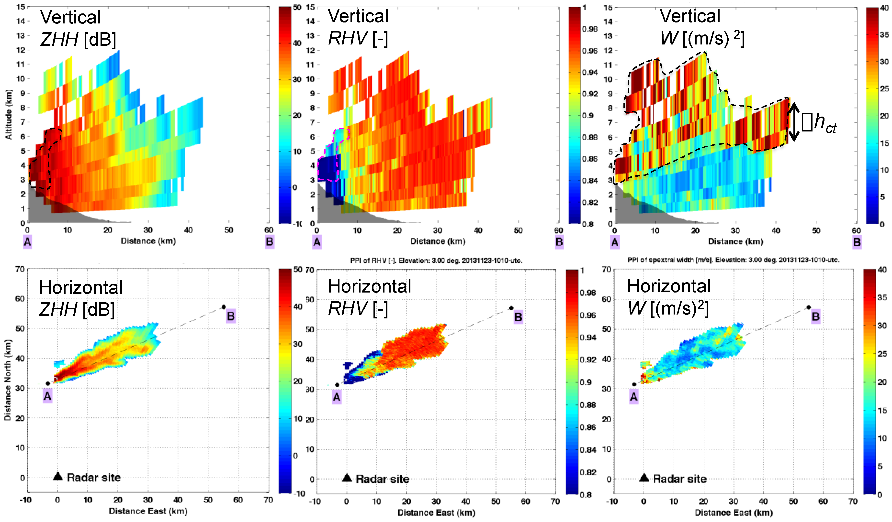
In this work, the measurements from the MSG-SEVIRI and Aqua-MODIS satellites were used to retrieve volcanic ash cloud parameters (Ma, AOD, Re) using the volcanic plume removal (VPR) algorithm [20,21].
SEVIRI is the primary instrument on board the EUMETSAT-MSG platforms. SEVIRI has 12 spectral channels with a nadir spatial resolution of 3 km (1 km for the high resolution HRV channel) and a repeat cycle of 15 min in full Earth scan mode or 5 min in rapid scan mode (only over Europe and North Africa). Data from the SEVIRI rapid scan aboard the MSG2 satellite (positioned at 9.5° E) were considered in this study.
MODIS is a multispectral radiometer on board the NASA Terra (EOS-AM) and Aqua (EOS-PM) polar platforms. MODIS has 36 spectral channels with a nadir spatial resolution from 250 m–1 km (1 km for the thermal infrared (TIR) channels). Terra’s orbit around the Earth is timed so that it passes from north to south across the Equator in the morning, while Aqua passes south to north over the Equator in the afternoon. Terra MODIS and Aqua MODIS view the entire surface of the Earth every 1–2 days.
The VPR procedure was designed for simultaneous real-time retrieval of volcanic ash and SO2 cloud parameters from TIR data. The volcanic cloud top altitude is the only input required at run time. The VPR method is easy to use and useful for monitoring active volcanoes, giving fast and reliable results [22]. The most time-consuming computations are anticipated in a preliminary phase during which the procedure is set-up for a given location (pressure, temperature and humidity profiles), surface characteristics (temperature and emissivity), ash type (refractive index and size distribution), volcanic cloud geometry (altitude and thickness) and sensor (response function). In this work, the Volz ash type [23] and log-normal size distribution were considered. The VPR procedure starts with the computation of a new image by replacing the radiance values in the region occupied by the plume with those obtained from a simple linear regression of the radiance outside the edges of the plume. The linear regression is performed considering the different surface contributions (these being clear sea, clear land or cloud) if land-sea and cloud masks are available. Thus, once the plume is removed, the new virtual image obtained shows an estimation of what the sensor on the satellite would have seen if the plume were not present. The two images, the original and the virtual one generated by removing the plume, allow estimation of plume transmittances for the TIR bands centred at about 11 and 12 μm (SEVIRI Channel Nos. 9 and 10, MODIS Channel Nos. 31 and 32) from which Re and AOD are retrieved. Finally, the ash mass is computed using the Wen and Rose [24] simplified formula. Within the APhoRISM project, an improved VPR version was developed to retrieve plume transmittance. In this improvement [25], the layer of atmosphere above the ash cloud is considered, as well as the thermal radiance scattered along the line-of-sight of the sensor.

3.2. X-Band Radar

The X-band radar system used in this work (DPX4) is permanently positioned at Catania airport (Sicily, Italy, 37.462° N, 15.050° E, altitude = 14 m), approximately 32 km away from the NSEC crater. DPX4 is part of four mobile systems of the National Department of Civil Protection, which is in charge of its maintenance and use.
The DPX4 system works at about 9.4 GHz (i.e., about a 3-cm wavelength), and it covers an area within a 160 km-wide circle, producing a data volume every 10 min. The data volumes consists of 12 maps in polar coordinates, which are obtained thanks to the 360° antenna revolutions and by pointing the antenna at different elevation angles relative to the horizon: specifically for DPX4 at 1°, 2°, 3°, 5°, 6°, 8°, 9.5°, 11.0°, 13.2°, 15.0°, 18.3° and 21.6°. For a given elevation angle, each map has 360 rays sampled at 1° in the azimuth and 200 m in the radial distance. Even though the radar data volumes are issued every 10 min, the actual time necessary to complete a volume acquisition is 5 min from the beginning of the acquisition time. This is an important aspect to consider when performing time collocations with other data sources. The DPX4 has a dual polarization and Doppler capability. Thanks to the former feature, there is the theoretical opportunity to investigate the predominant shape, orientation and homogeneity of the detected ash particles while the latter gives the possibility of obtaining information on average particle velocity and the dispersion around the mean.
Among the available radar output variables, this work makes use of the co-polar radar reflectivity (ZHH) cross-correlation coefficient (RHV) and velocity dispersion (W). ZHH (dB) is mostly related to particle size, since larger sized particles tend to produce a stronger power return back to the radar receiver. RHV (unitless) is the modulus of the correlation coefficient between horizontal-polarized (H) and vertical-polarized (V) signals, and it describes the target heterogeneity within the radar resolution cells, while W (m2/s2) is an indication of the diversity of the particle radial velocities. For a robust theoretical background in the meaning of radar variables, see Bringi et al. [26], and for exploitation of radar polarimetry in relation to ash clouds, see Vulpiani et al. [27], Montopoli et al. [28] and Crouch et al. [29].
The ash products derived from the DPX4 radar fall into two categories: microphysical products and geometrical products. The former include Ca, Ma and Re, while the latter include hct and Δhct. The volcanic ash radar retrieval (VARR) procedure, developed in Marzano et al., 2006 [30], and subsequently applied to polarimetric data by Vulpiani et al. [27] and Montopoli et al. [28], is used to define the microphysical characteristics of an ash cloud from radar data. The VARR is based on forward electromagnetic simulations of ash particles in the microwave region assuming a Gamma size distribution model of oblate particles with the random orientation, axis ratio, permittivity and canting angle as specified in [31,32]. Next, the forward simulations are used to parameterise Re and Ca as a function of reflectivity ZHH for a set of predefined ash categories assigned to each radar grid cell through a Bayesian classification step. Ma is calculated by integrating the estimated concentration Ca, along the vertical radar resolution cells. The top of the ash cloud, hct, is derived by extracting the position of the highest radar resolution cells where an appreciable signal is detected. Conversely, the Doppler width, W, together with correlation of H- and V-polarized radar signals, named RHV, are used to infer the thickness Δhct. The rationale behind the use of W for an estimation of Δhct is that it is a good indicator of turbulence effects, which are expected to be predominant in the forcing region of the rising column (i.e., updraft zone), as well as in the area where the plume is transported by cross winds (i.e., advection zone). In order to eliminate the area affected by the updraft from the analysis, but to retain that of the advection zone, which is of interest for the definition of Δhct, the radar measurement RHV is used. It is lower in the region of the updraft, because, above the vent, the reshuffling of heterogeneous-sized particles can cause a wider decorrelation between the H and V channels. Thus, excluding the radar pixels where RHV is low allows identification of the advection zone and, so, an estimation of the thickness of the propagating cloud as seen by the radar.

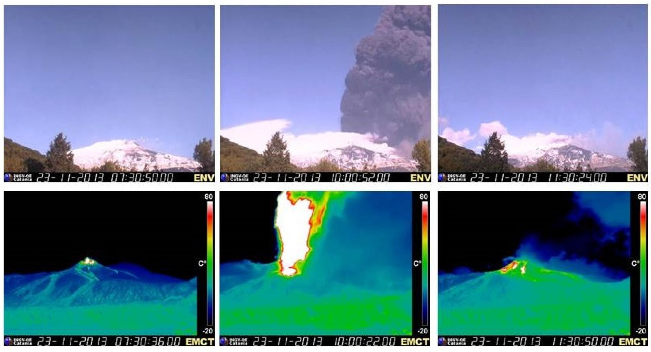
4. Satellite and Ground-Based Volcanic Ash Retrieval Results

In this section, the SEVIRI, MODIS and DPX4 volcanic ash retrievals are described separately. The data integration is presented in Section 5.

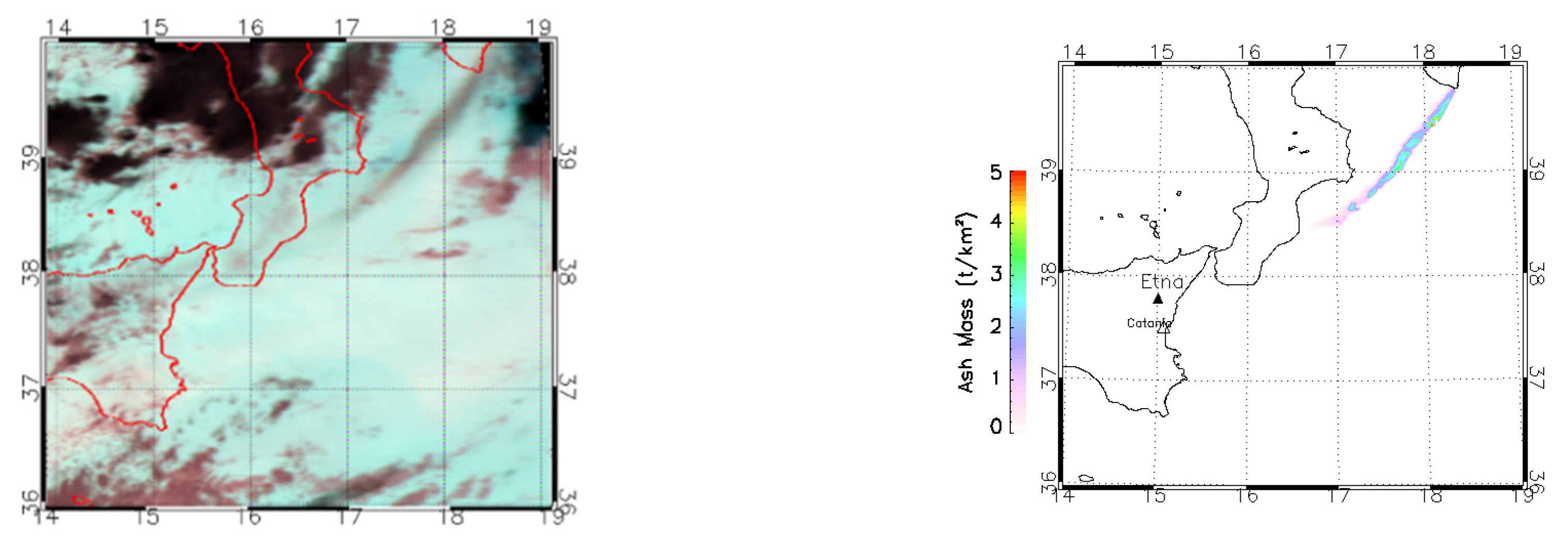
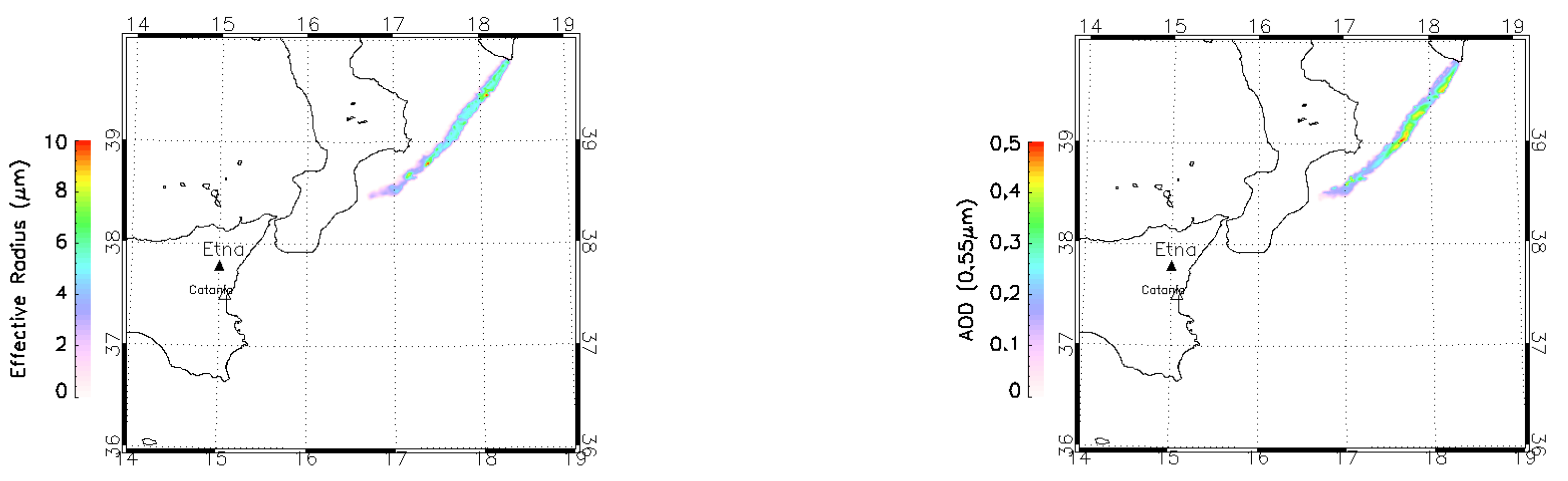
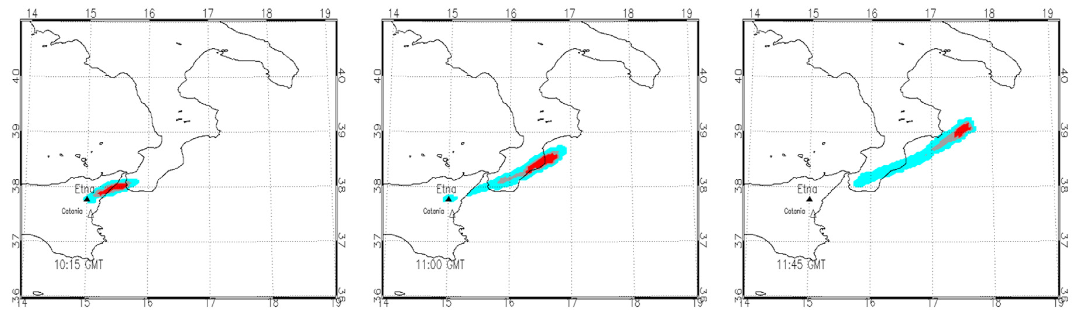
4.1. Satellite Ash Retrievals

As stated in Section 3.1, the only input required to run the VPR retrieval procedure is the volcanic cloud top altitude. This parameter is computed using two different approaches: dark pixels and ash centre of mass tracking.
The dark pixels procedure is based on a comparison between the mean brightness temperature at 11 μm of the volcanic ash cloud’s most opaque pixels, with an atmospheric temperature profile collected near (in time and space) the area of interest. Since it is reasonable to assume that the selected pixels are not completely dark, the temperature of the cloud top is set two degrees lower [9,33]. A reference temperature was defined using the National Centers for Environmental Prediction (NCEP)/National Center for Atmospheric Research (NCAR) reanalysis profile [34] (resolution 2.5° × 2.5°) centred on the Etna volcano and collected at 12:00 UTC.
The ash altitude retrieval based on ash centre of mass tracking is computed by comparing the wind speed, obtained by following the ash centre of mass using the series of SEVIRI images, with the wind atmospheric profile of the area of interest (the main hypothesis is that the speed of the volcanic cloud coincides with the wind speed at the volcanic cloud altitude). The upper panels of Figure 2 emphasize the position of the ash cloud centre of mass considering three SEVIRI images at different times. Since, at this stage, it is not important to have an accurate quantification of the amount of ash, but only a reasonable representation of the spatial pattern of the ash cloud in order to detect its centre of mass, the ash maps were obtained using a default value of plume altitude fixed to 10 km. In the same figure (bottom left panel), the distance and direction of the volcanic cloud centre of mass retrieved using the different SEVIRI images are plotted. The wind speed is computed between 10:15 and 12:30 UTC, where a linear trend is obtained, and its value is estimated to be 38.2 m/s. This time interval was selected because before 10:15, the lava fountain was still present, and the centre of ash mass was in approximately the same position over the vent, while after 12:30 UTC, the volcanic cloud was so diluted, that its automatic detection became difficult. The computed wind speed was then compared with the mean NCEP/NCAR wind speed profile at 12:00 UTC obtained considering the profiles centred on Etna at 39.5° N–17.5° E (see the bottom right panel of Figure 2). This area included most of the volcanic cloud at that time.
Figure 2. Top panels: ash cloud centre of mass at different times. Bottom left plot: distance (red squares) and direction (blue triangles, defined as the direction from which the wind was blowing) of the volcanic ash cloud centre of mass considering the different SEVIRI images. Bottom right plot: comparison between the wind speed retrieved (vertical dashed line) with the National Centers for Environmental Prediction (NCEP)/National Center for Atmospheric Research (NCAR) mean wind speed profile extracted in the area occupied by the volcanic cloud (red solid line). The dashed blue lines represent the standard deviation of the mean NCEP/NCAR wind speed profile.
Remotesensing 08 00058 g002
Figure 3 summarizes the results of the volcanic cloud altitude obtained using the two approaches described above and applied to SEVIRI data. Dark pixels were found in six images (09:45, 10:00, 10:15, 10:30, 10:45 and 11:00 UTC) (see the black diamond symbols), and the volcanic cloud altitudes retrieved from the centre of mass tracking were not the same as the two results found at about 7 and 11 km (see the orange diamond symbols). The retrieval errors were computed from the standard deviation of the brightness temperature obtained from the dark pixels and from the standard deviation of the mean NCEP wind speed.
Figure 3. Volcanic ash cloud altitudes computed from SEVIRI images using the dark pixel (black diamonds) and centre of mass (orange diamonds) procedures. The curve of the red diamonds represents the volcanic cloud altitude used for all of the SEVIRI image processing.
Remotesensing 08 00058 g003
The red diamonds in Figure 3 represent the volcanic cloud altitudes used for all of the SEVIRI image elaborations. Since no dark pixels were found after 11:00 UTC, the altitude attributed to the 11:15, 11:30 and 11:45 UTC images is the value found at 11:00 UTC. Moreover, after 12:00 UTC, the upper value obtained from the ash centre of mass tracking was considered. Note that the lower altitude value (7 km) found by centre of mass tracking was discarded from this analysis. This was motivated by the consideration that, according to the particle velocity limit equation, spherical particles of 20 μm in diameter (the maximum diameter of particles detectable by SEVIRI in the TIR spectral range) fall at about 1.2 cm/s, i.e., in 1 h, the vertical fall is approximately 43 m. This means that starting from a peak altitude of about 12 km at 10:30 UTC, these particles could not reach an altitude of 7 km one hour later.
These altitude values were used to compute the ash parameters (Ma, Re and AOD). Figure 4 shows the total ash mass, the mean effective radius and the mean aerosol optical depth for the series of SEVIRI images. For each image, the total ash mass (t) was obtained by adding all of the pixels’ ash masses (computed by multiplying the pixel ash mass loading (t/km2) by the pixel size (km2)), while the mean effective radius and mean aerosol optical depth are the mean values of the Re and AOD maps. The error bars are derived from Wen and Rose [24] and Corradini et al. [35].
Figure 4. Volcanic ash Ma (left panel), mean Re (middle panel) and mean AOD (right panel) for the series of SEVIRI images.
Remotesensing 08 00058 g004
Note that the dark pixel procedure could not be used to retrieve the volcanic cloud altitude from MODIS data collected at 12:45 UTC, because the ash cloud was too transparent (no opaque pixels present). Consequently, the volcanic cloud altitude retrieved from SEVIRI at the same time was used to process the Aqua-MODIS image using the VPR approach. Figure 5 shows the MODIS RGB image using Channels 28, 29 and 31 and the retrieved ash parameter maps. The total mass, mean Re and mean AOD are 7541 ± 3016 t, 5.64 ± 2.2 μm and 0.12 ± 0.05, respectively. These values are in agreement with those obtained from the SEVIRI image collected at the same time (4971 ± 1988 t, 5.12 ± 2.0 and 0.18 ± 0.07, respectively, for total mass, mean Re and mean AOD). The largest difference was found for total ash mass and was mainly due to the different sensitivity of the SEVIRI and MODIS instruments, particularly significant in the case of diluted clouds (the noise equivalent temperature difference (NEΔT) of the SEVIRI channels used for the ash retrievals is more than double the NEΔT of the corresponding MODIS channels).
Figure 5. RGB image (R:28, G:29, B:31, upper left panel), volcanic ash Ma (upper right panel), Re (lower left panel) and AOD (lower right panel) for the MODIS image collected at 12:45 UTC.
Remotesensing 08 00058 g005aRemotesensing 08 00058 g005b

4.2. DPX4 Ash Retrievals

Following the VARR methodology described in Section 3.2, some of the ash plume features were extracted for the case study of 23 November 2013. The radar data consists of volume acquisitions providing a three-dimensional view of the scene within the radar coverage. Figure 6 shows an example of a data volume in terms of vertical cross-sections and planar maps (upper and lower row panels, respectively). The vertical cross-sections were extracted along the plume axis A-B (see the bottom panels of Figure 6). Three variables are shown from left to right: the radar reflectivity, ZHH, the cross-correlation coefficient, RHV, and the Doppler spectrum width, W. The pattern of ZHH is used to retrieve the top altitude of the ash cloud and the particle size distribution.
Figure 6. Upper panels: vertical cross-sections, along the prevailing wind direction A–B, of the radar variables used in this work sampled at 10:10 UTC on 23 November 2013 from the DPX4 radar in Catania (Sicily, Italy); lower panels: horizontal radar maps at a 3° radar antenna view angle from the horizon. The dashed lines in the top left and middle panels highlight the areas probably affected by particle updraft, whereas the area contoured in the top right panel marks the region most affected by cross winds.
Remotesensing 08 00058 g006
As a rule of thumb, larger ZHH values generally indicate the presence of larger particles within each radar resolution cell; thus, the behaviour of ZHH in the left panels of Figure 6 indicates a variable spatial distribution of ash particle size. In the same figure, the dashed lines in the top left and middle panels highlight the areas probably affected by particle updraft, whereas the area contoured in the top right panel marks the region of higher values of Doppler spectrum width, which can be a sign of particle updraft or plume transportation by horizontal cross winds.
The quantification of particle size distribution is shown in Figure 7, left panel, in terms of the number density distribution. The particle size distribution retrieved by the radar is in units of number of particles·m−3·mm−1, while the number density distribution is expressed in number of particles·m−3. The number of particles per unit of volume is estimated by multiplying the particle size distribution by its particle radius resolution bin (Δr) in mm. In Figure 7, the temporal variation in the average gamma-modelled number density distribution for each radar volume is drawn. The number density distributions show a significant variation over the range of average sizes from 25 μm–2 mm, which is consistent with the radar detection limit investigated by theoretical models in previous studies [32]. However, particle sizes lower than 25 μm are outside the radar's detection limit, and so, the curves of the multi-temporal gamma-modelled distributions coincide in that particle range. The middle panel of Figure 7 shows the cloud top altitude as a function of the distance along the transect A-B for the acquisition times when the radar detected a signal higher than a minimum threshold, i.e., ZHH > −10 dBZ. The pulsating behaviour of the volcanic source emission is evident from the cloud top variability at distances closer to the volcano vent. From the radar perspective, as time goes on, the cloud top decreases, and its leading edge progresses leaving the volcano summit. This figure shows that the “coarse” particles tend to fall out within the first 60 km from the vent. The discrepancy between the SEVIRI ash cloud altitude retrievals using the dark pixels procedure (see Section 4.1), and the altitude retrieved by the DPX4 system is because these the systems are looking at different particles: fine for SEVIRI and coarse for DPX4. The right panel of Figure 7 shows the total mass obtained as the integral of the radar-derived ash mass concentration over the whole volume affected by the ash plume. It is noted that the magnitude of the microwave radar-derived total ash mass is 102 larger than that obtained by infrared retrievals. This can be explained by the different sensitivities to the particle sizes seen by microwave and infrared sensors.
Figure 7. DPX4 retrievals. Left panel: gamma-modelled ash number density distribution; middle panel: ash plume maximum altitudes as a function of the distance from Mt. Etna for the different DPX4 acquisition times (UTC); right panel: total ash mass of the ash plume.
Remotesensing 08 00058 g007
The final parameter estimated by radar is ash cloud thickness. It is derived using the Doppler spectrum width, W. Figure 6, upper middle and right panels, shows a clear example of the use of W and RHV as a proxy for ash cloud thickness. From these panels, W is larger than 25 m/s2, and RHV > 0.95 identifies the portion of the cloud that is transported by lateral winds. The cloud thickness seen by radar is variable in space, since in the areas closer to the vent, the cloud top altitude is mainly driven by the pulsating forcing updraft. Thus, it is more convenient, with a view toward multi-sensor integration plans and for an analysis of cloud thickness, to consider the leading edge of the transported ash cloud, this being the cloud portion filled by finer ash particles. By isolating the farthest area of the ash cloud from the volcano summit and considering the instant at which the cloud top seen by the radar is showing a homogenous decreasing trend (i.e., 10:10 UTC), the cloud thickness is estimated on average between 1.5 km and 3 km (see Figure 6, upper right panel). The uncertainty in cloud thickness is due to the radar's vertical resolution, which is variable with radar distance. At the leading edge of the plume observed at 10:10 UTC (i.e., about 40 km away from the radar’s position), the thickness was ±0.4 km. Effects due to variations in the refractive index bending the radar ray path are not considered, since they are expected to be negligible within a 40-km path.

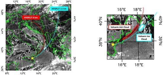
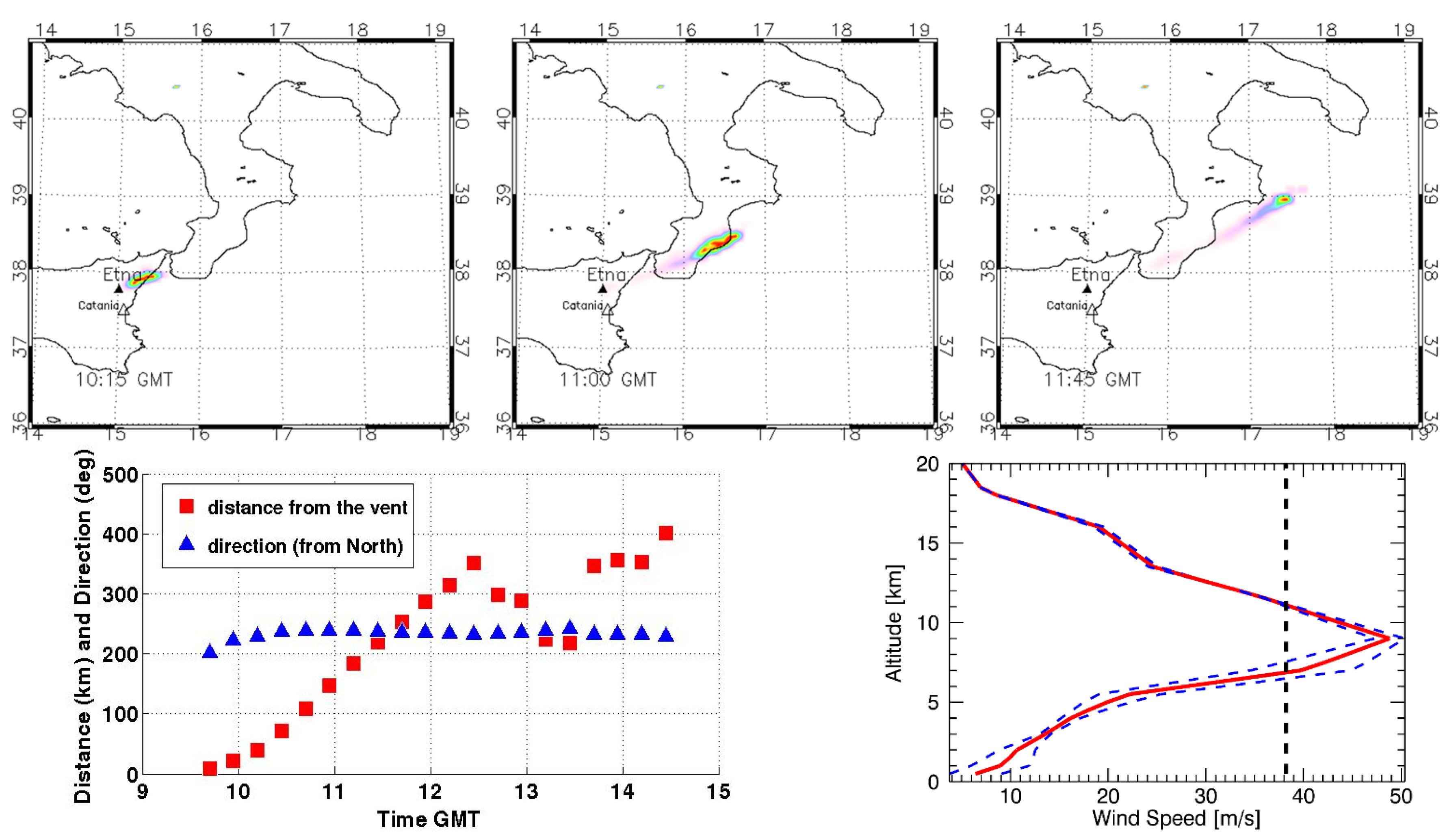
5. The Multi-Sensor Approach

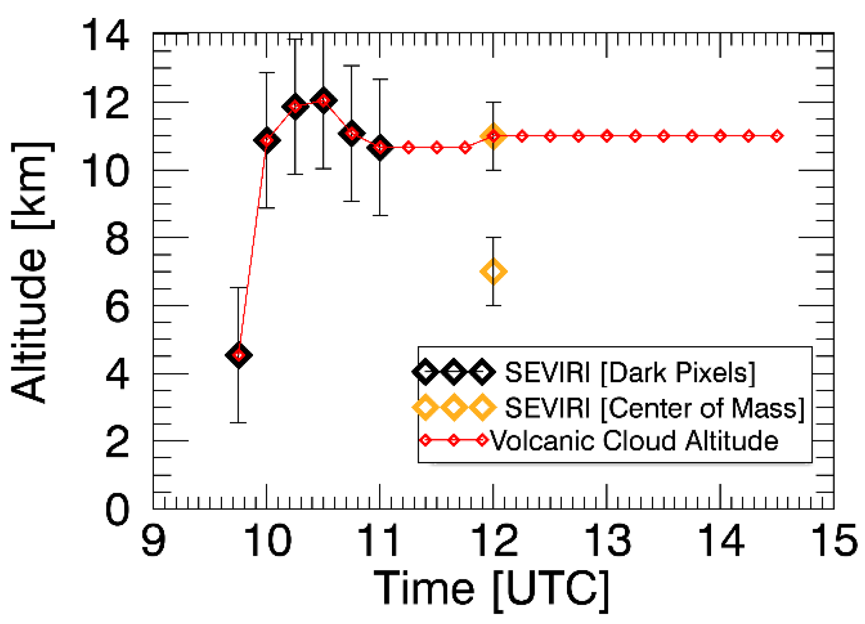
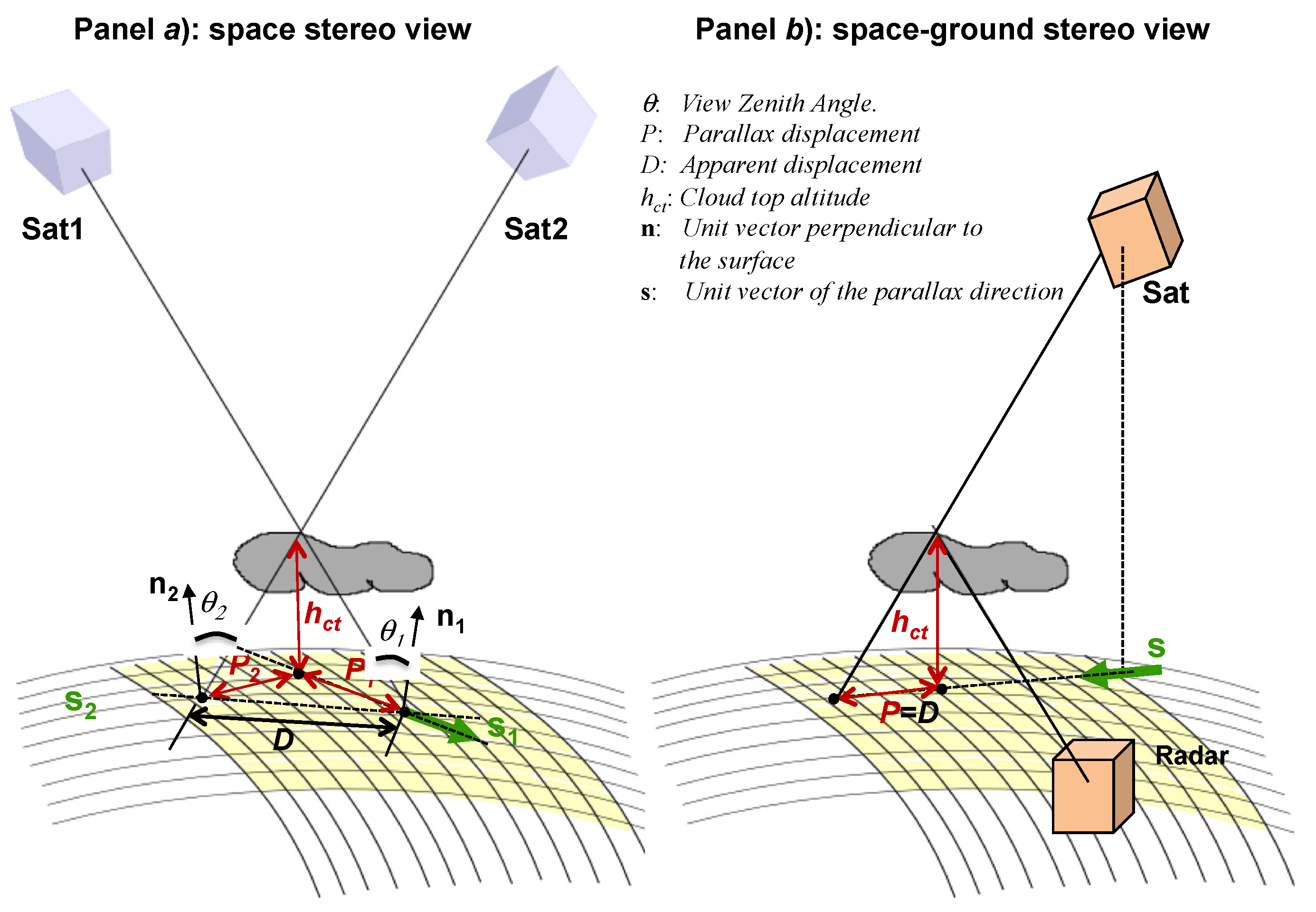
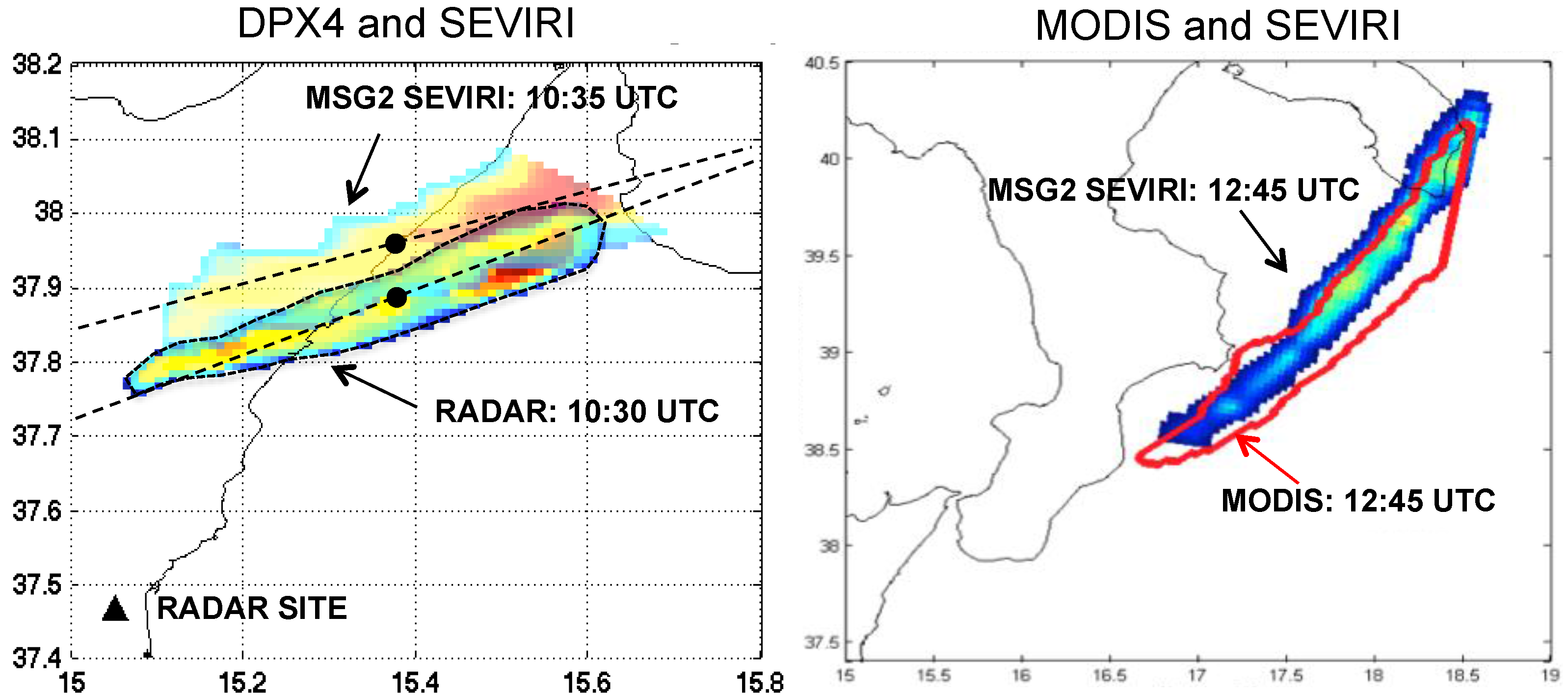
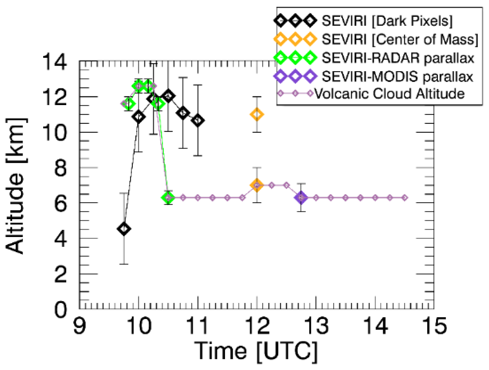
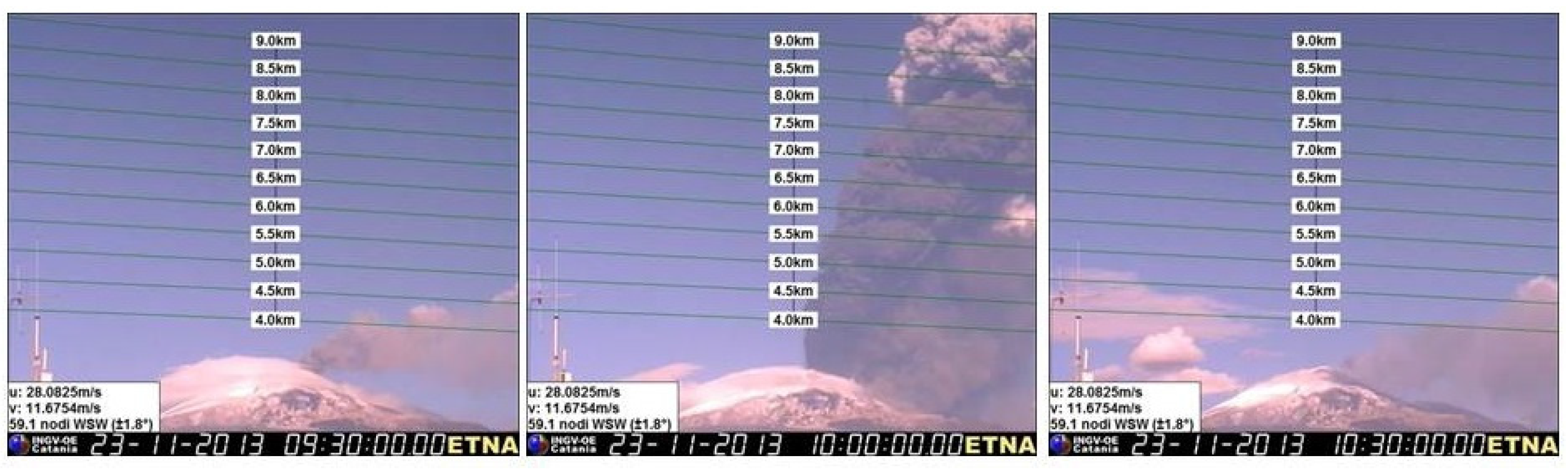
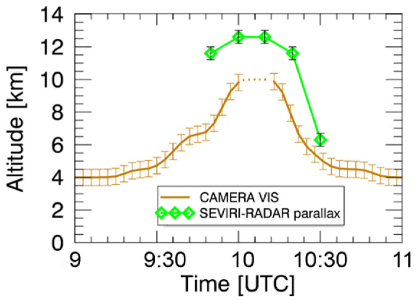
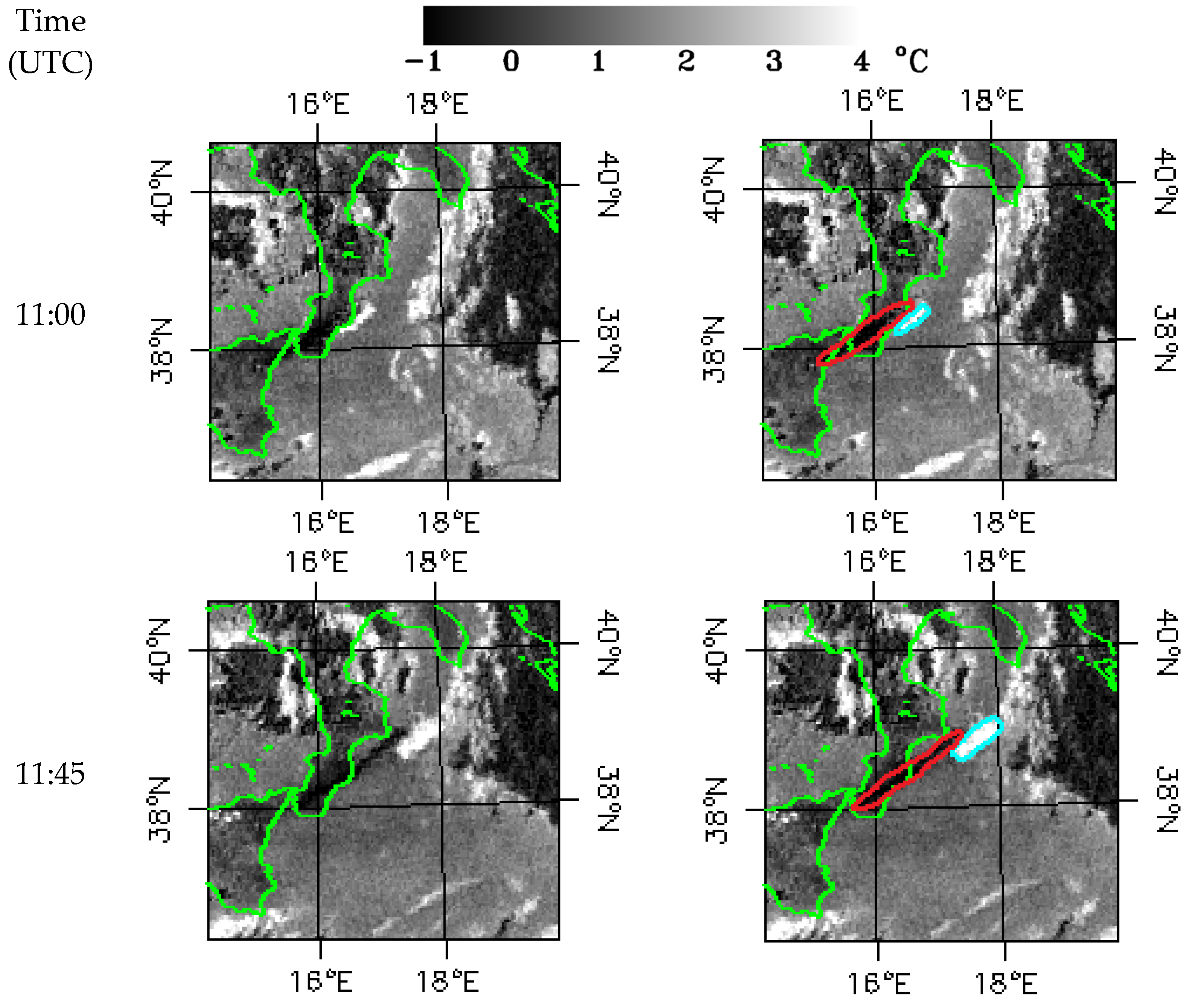
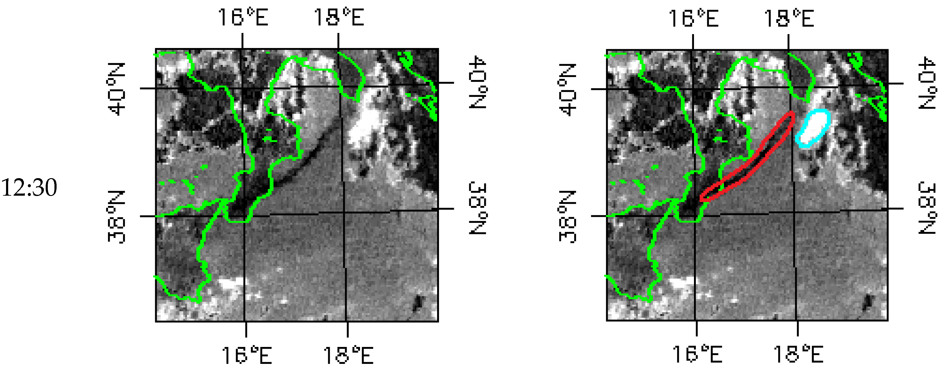
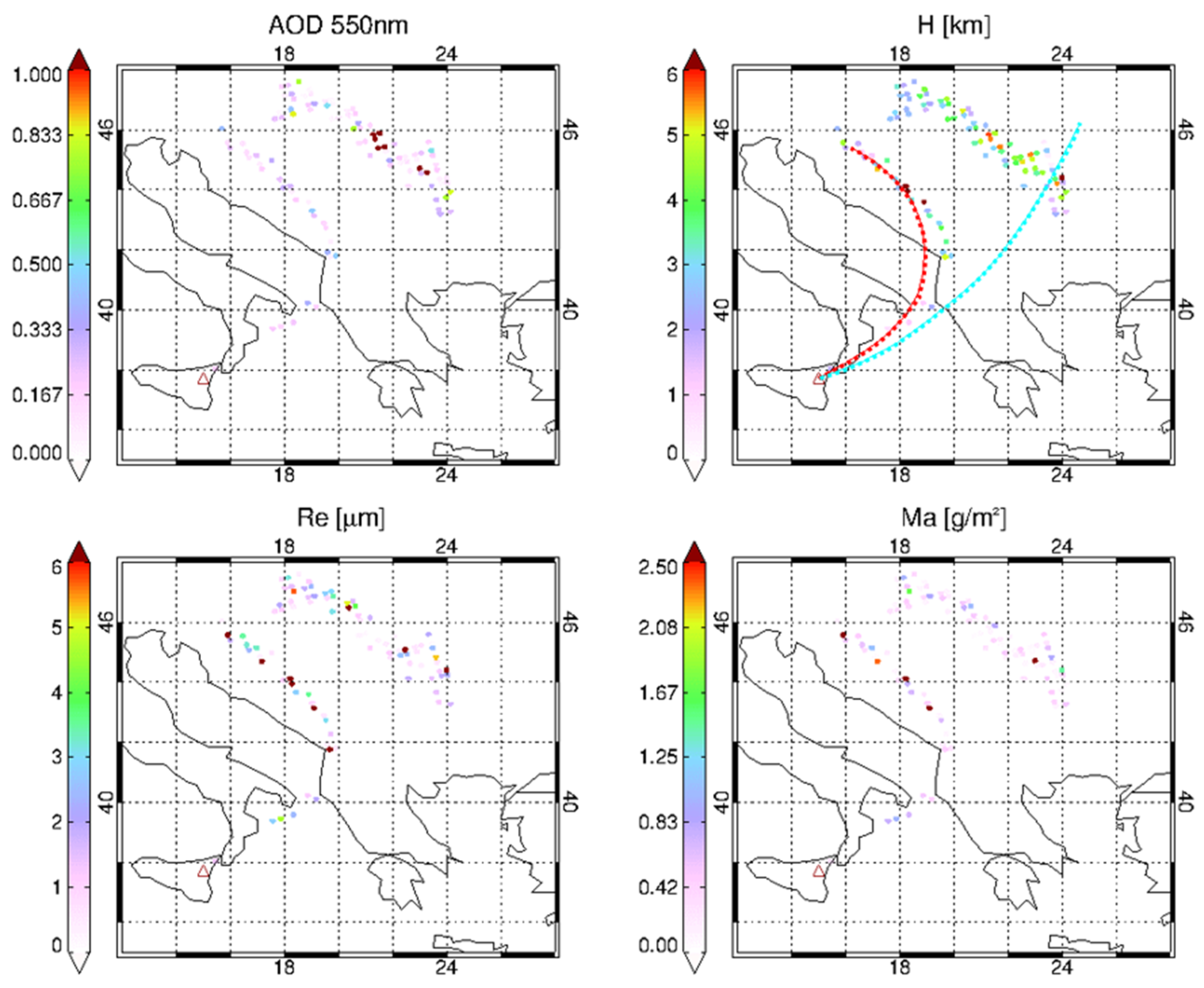
5.1. Volcanic Cloud Altitude

Identification of the ash cloud top altitude is the only input parameter needed to run the VPR procedure, which quantifies the physical characteristics of the ash cloud using SEVIRI and MODIS data. The exploitation of parallax effects [36] can in principle be used to quantify the cloud top altitude, and it represents an additional tool along with other methods, like centre of mass tracking and dark pixel identification, described in Section 4.1.
Parallax can be defined as a displacement of the apparent position of a target on a reference plane, so that it is viewed along two different lines of sight (i.e., two different view angles) [37]. In the case of atmospheric clouds, if we know the geometry by which two sensors view the same cloud along two different lines of sight (and their acquisitions are nearly simultaneous), it is possible to estimate the displacement of the cloud from its real position and establish the target’s altitude by trigonometric calculation.
The left panel of Figure 8 (panel a) shows a general configuration with two satellite platforms observing the same cloud from different angles, while the right panel Figure 8 (panel b) shows an example of combining a ground station view and a satellite. The present study used both the configurations shown in Figure 8 for the SEVIRI-MODIS (panel a) and SEVIRI-DPX4 (panel b) nearly simultaneous acquisitions. For the more general configuration of Figure 8 (SEVIRI-MODIS), the cloud top height hct is formalised by the following equation:
h c t = P 1 / t g ( θ 1 ) = P 2 / t g ( θ 2 )
where tg1) and tg2) are the tangent of the view zenith angles of the two satellites (known) and the parallax shifts, P1 and P2, can be derived from the apparent displacement (D) between the footprints of the cloud, which are differently projected on the ground when seen from two satellites. Once D is estimated and the view azimuth angles of the two satellites are known, P1 and P2 are calculated geometrically (i.e., applying the law of sines). In the configuration shown in panel b (SEVIRI-DPX4), Equation (1) is simplified, since only one side needs to be considered.
Figure 8. Parallax configurations. Left panel (panel a): two satellite sensors view the same target along two different lines of sight; right panel (panel b): a satellite and a ground station form the parallax view.
Remotesensing 08 00058 g008
It is worth noting that although the microwave radar provides the quantity hct directly, the hct value derived by the radar might not be consistent with that derived by the infrared sensors due to their different sensitivity to particle sizes. For this reason, the radar can miss the part of the cloud with the finest particles, which presumably occupies the area above the hct derived by the radar. The net result of this could be an underestimation of the ash cloud altitude seen by the ground radar. The exploitation of the parallax approach is a way to overcome this issue by comparing the horizontal spatial patterns of the ash cloud seen by the microwave ground radar with the observations of the infrared satellite radiometers. The differing spatial pattern of the ash cloud seen by the two sensors due to their different particle size sensitivity is attenuated, because it is limited to the diluted horizontal edge of the cloud, leaving the bulk of the cloud unaffected.
As stated before, for the case study on 23 November 2013, hct was calculated in both configurations of Figure 8 using the SEVIRI-MODIS and SEVIRI-DPX4 sensors. Image cross-correlation analysis was applied between the ash plume horizontal patterns derived from the two pairs of nearly simultaneous sensor acquisitions, estimating D and then calculating hct (the mean angles θ in the volcanic cloud were used).
The cross-correlation technique establishes which average displacement provides the highest correlation between the clouds seen by the selected pair of sensors. Before implementing image cross-correlation, an image interpolation is applied to homogenize the available acquisitions on the same common grid. The finer grid is chosen for each pair of sensors analysed (i.e., the 1-km MODIS and the resampled 1-km DPX4 grid). Additionally, the cross-correlation is performed on normalized values, in order to make the outcome of the correlation analysis more sensitive to the horizontal footprint pattern of the ash cloud and less sensitive to differences in the estimated values. The normalization values are fixed, for each acquisition instant, to the maximum intensity (in space) of the total ash mass estimates from each sensor, thus reducing the dynamic range of each estimate in the [0,1] interval. The choice to normalise the ash mass loading estimates from MODIS or SEVIRI and DPX4 before performing correlation makes the ash mass more homogeneous. After normalization, the correlation analysis is more sensitive to horizontal variations in the mass loading estimates than to differences in vertical stratification observed by the two sensors. This makes the final result less sensitive to the process of particle sorting and differences in particle size, which are typically more pronounced along the vertical direction than the horizontal.
Note that the parallax P is defined as the displacement along the direction s of the parallax (see Figure 8). The cloud displacement established from the cross-correlation analysis was then constrained to lie along the direction s. This is why the method was named “constrained cross-correlation”. It is obvious that in the SEVIRI-DXP4 configuration, the direction s coincides with the satellite view azimuth angle, while in the MODIS-SEVIRI configuration, the direction s was determined by choosing the one that satisfies both of the equalities in Equation (1). Table 3 lists the values of the ash cloud top altitudes derived applying the constrained cross-correlation to the time-collocated acquisitions of SEVIRI, MODIS and DPX4 for the Mt. Etna event of 23 November 2013.
Table 3. Values of cloud top heights, hct, derived using constrained cross-correlation analysis of various pairs of sensors and acquisition times for the Etna event of 23 November 2013.
SEVIRI Nominal Time (UTC) (Effective Time in Etna Area (UTC)DPX4 Time Intervals (UTC)hct ± Δhct (km)
09:50 (09:52:30)09:50–09:5511.6 ± 0.4
10:00 (10:02:30)10:00–10:0512.6 ± 0.4
10:10 (10:12:30)10:10–10:1512.6 ± 0.4
10:20 (10:22:30)10:20–10:2511.6 ± 0.4
10:30 (10:32:30)10:30–10:356.3 ± 0.4
SEVIRIMODIS
12:45 (12:47:30)12:45 (12:47:00)6.3 ± 0.8
An example of nearly simultaneous acquisitions of SEVIRI-DPX4 and SEVIRI-MODIS is shown in Figure 9, where the parallax displacement is evident. In Table 3, the values of the cloud top altitudes extracted by the constrained cross-correlation range from 6.3 km–12.6 km with a decreasing trend over time. The higher cloud top altitude values registered before 10:20 UTC are probably caused by ongoing volcanic emissions forcing the plume to rise due to powerful updraft forces. After 10:20 UTC, emissions ended, as confirmed by the radar acquisition, and at 10:30 UTC (i.e., last time frame in which ash was detected by the radar), the estimated cloud top was around 6.3 km. This value is surprisingly consistent with that obtained 2.25 h later when the MODIS and SEVIRI parallax is extracted at 12:45 UTC and the plume had travelled several hundred kilometres away from the volcanic vent. A cloud top altitude value of 6.3 km thus appears to offer the closest agreement between the multi-sensor observations analysed.
Figure 9. Example of parallax displacement when retrievals from SEVIRI and DPX4 radar (left), and MODIS and SEVIRI (right) are compared to each other at nearly simultaneous acquisition times.
Remotesensing 08 00058 g009
Figure 10 shows the volcanic cloud altitudes computed from the SEVIRI images (see Section 4.1) and the values obtained from the parallax computations.
Figure 10. Volcanic cloud altitude retrieved from SEVIRI images, SEVIRI-DPX4 and SEVIRI-MODIS parallaxes. The light purple curve represents the volcanic cloud altitude obtained from the multi-sensor integration.
Remotesensing 08 00058 g010
The light purple line represents the volcanic ash cloud altitude time series, retrieved using the multi-sensor approach. The SEVIRI-DPX4 and SEVIRI-MODIS parallaxes indicate (from 10:30 UTC onwards) volcanic ash cloud altitudes significantly lower than the values obtained from the analysis of the SEVIRI images (see the red curve in Figure 3). In this case, the upper value obtained from the ash centre of mass (orange diamond) was discarded. The latter analysis, and the previous analysis based on dark pixels, suggest the presence of two cloud layers, an upper layer composed of a mixture of ash, ice and water particles and a lower layer only of ash (for a detailed analysis, see Section 6). The DPX4 radar does not detect the upper cloud after 10:30 UTC, probably due to a combination of causes: (i) small airborne particles beyond the range of radar detection; (ii) the permittivity constant of ice is smaller than that of water and ash, thus leading to a weaker backscattered radar signal; and (iii) a diluted cloud leading to a low concentration of particles and a reduction in the volume contribution to the backscattered radar signal.

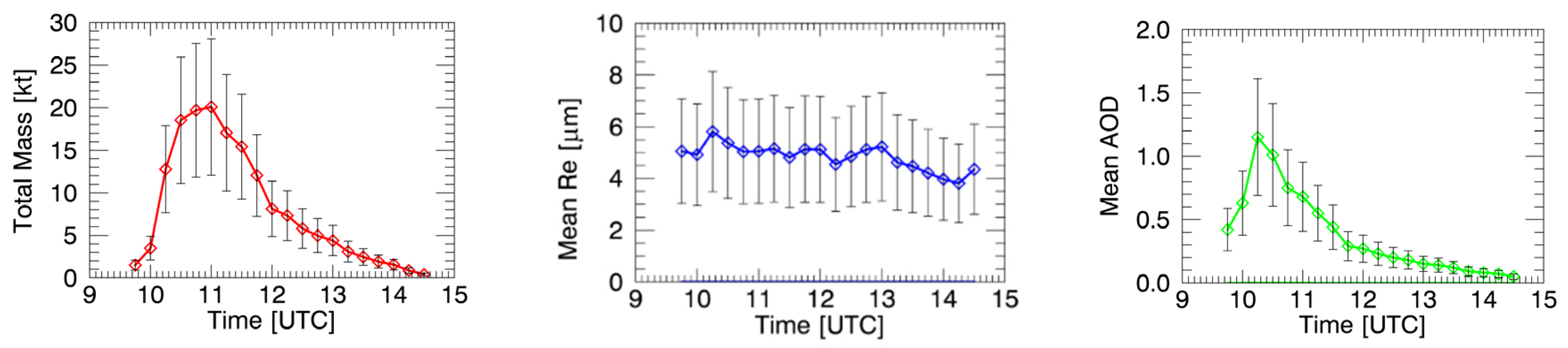
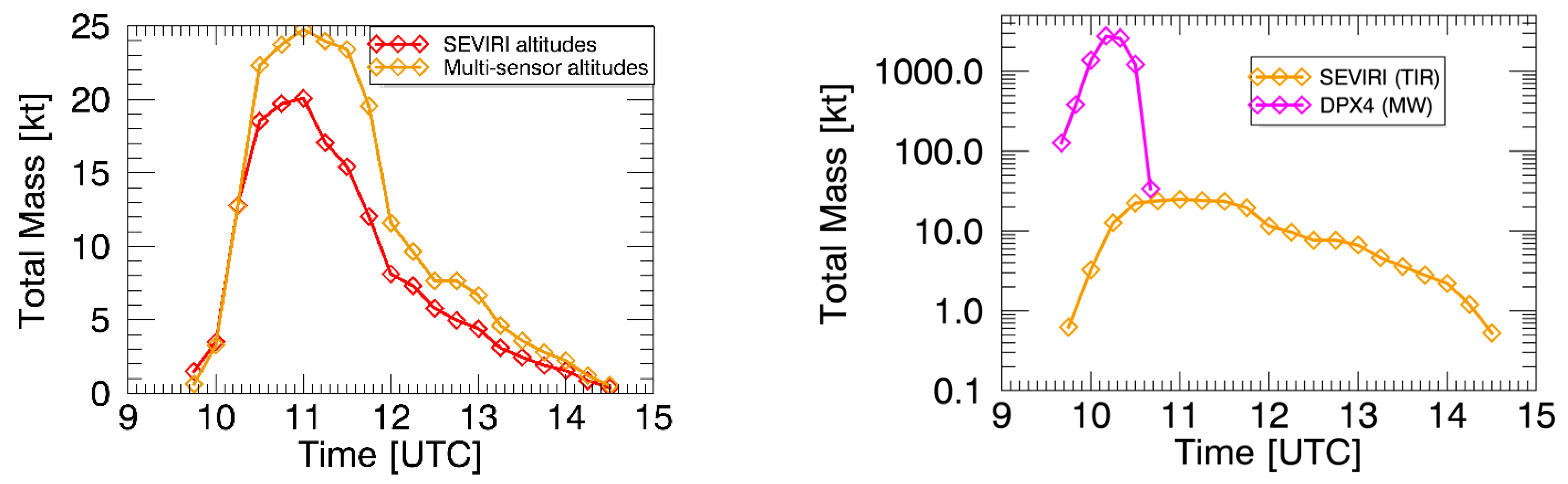
5.2. Total Ash Mass Emitted and Ash Concentration in the Atmosphere

In the light of the new findings discussed in the previous Section 5.1 and because the ash retrievals procedure used for the SEVIRI data processing depends only on cloud altitude, the SEVIRI images were reprocessed using the volcanic cloud altitude values obtained from the image integrations. The ash retrievals produced using the integrated cloud altitude values are significantly greater than the initial results obtained using only the SEVIRI altitude estimation (see Figure 11, left panel). The mean percentage differences between the Ma, Re and AOD values retrieved before and after integration were about 30%, 10% and 20%, respectively. By using the integrated volcanic ash altitude, also the MODIS retrievals are carried out. The percentage differences between the values obtained before and after the integration reflects the same differences found for SEVIRI. The right panel of Figure 11 shows the retrieved SEVIRI and DPX4 ash masses. As expected, the finest ash mass particles (0.5–10 μm) that characterize the ash cloud far from the vents (retrieved from SEVIRI in the TIR spectral range) make up only a few percent (1%–2%) of the total mass emitted from the volcano (retrieved from DPX4). Also notable is the continuity in the temporal evolution of the total ash mass. During the initial stages of an eruptive event, most of the ash mass is coarse particles that obviously fall down very quickly, producing a steep decrease in the ash mass (Figure 11, right panel, violet curve). During the same period, the finest fraction of emitted particles is increasing, reaching a plateau once the coarser particles have fallen out (yellow curve in the same panel). In subsequent stages, the total ash mass continuously decreases as the cloud propagates downwind and dilutes.
Figure 11. Left panel: SEVIRI ash masses retrieved before (red curve) and after (yellow curve) the multi-sensor approach; Right panel: SEVRI and DPX4 ash masses comparison.
Remotesensing 08 00058 g011
The volcanic ash concentration can be obtained by dividing the SEVIRI ash mass (retrieved using the volcanic cloud altitude established using the multi-sensor approach) with the ash thickness retrieved from DPX4 measurements (3 km). The concentration is used to define a classification map following the EASA guidelines (see Section 1). Figure 12 shows ash classification maps for some SEVIRI images where low, medium and high concentrations are colour-coded in cyan, grey and red, respectively.
Figure 12. Classification maps for the ash concentration following the European Aviation Safety Agency (EASA) guidelines. Low contamination (cyan); medium contamination (grey); high contamination (red).
Remotesensing 08 00058 g012
As regards the ash mass retrievals, the maximum difference between the ash classification areas computed before and after the multi-sensor approach is about 40% (i.e., the low, medium and high contamination areas, computed with the volcanic cloud altitude retrieved from the multi-sensor approach, are greater by up to 40% compared to the same areas computed using the volcanic cloud altitude obtained using only the SEVIRI cloud altitude estimation).

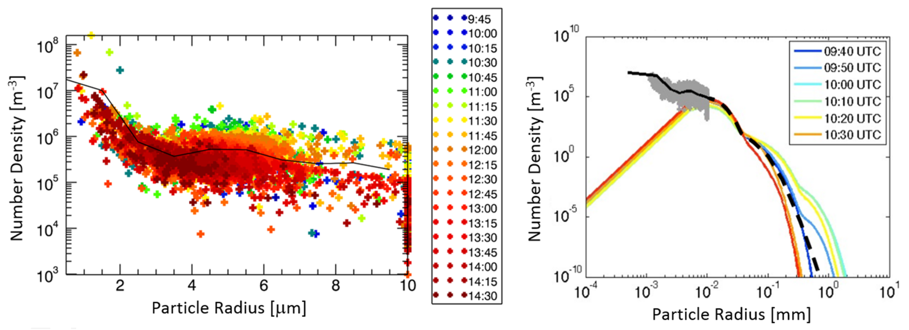
5.3. Particle Number Density

Knowledge of the SEVIRI ash concentration and mass enables calculation of an effective particle number density, ne. Under the assumption that for each SEVIRI pixel, the plume is composed of particles having the same size as the effective radius, the effective particle number density is computed by dividing the ash concentration (kg/m3) by the ash mass of the pixel (kg). The latter quantity is computed by multiplying the particle volume (m3) by the particle density (g/m3). A particle density value of 2.6 × 10³ (kg/m3) is used, while the volume is computed from 4/3 π Re3 (m3), where Re is the effective pixel radius. Note that ne is undoubtedly influenced by the choice of size distribution, but considering the assumption of monodispersed particles, for which only a single value of the distribution is sampled, the effective particle number density probably does not vary significantly with the size distribution shape.
The left panel of Figure 13 shows ne computed from SEVIRI data, while the right panel shows ne derived from both SEVIRI (grey shaded area) and DPX4 measurements (the dashed curve represents the average trend for the MW retrievals). With all of its intrinsic limitations, such a computation is important, because it gives an indication of the complementarity between the MW and TIR retrievals. In fact, the estimations carried out by these two different instruments, working at different spectral ranges, gives comparable results in a contiguous region around 10 μm.
Figure 13. Left panel: effective number density computed from the SEVIRI images. The solid black line represent the mean value. Right panel: same as the left panel (grey shaded area), but including the DPX4 retrievals (the dashed curve is the radar average).
Remotesensing 08 00058 g013

6. Products Validation

The retrieved volcanic ash cloud altitude, thickness and total mass are compared to the measurements obtained from the ground VIS camera, the IASI satellite, the HYSPLIT model forward trajectories and tephra deposits.

6.1. Volcanic Cloud Altitude

Quantitative height estimations from ground-based images are not very common, with few examples available in the literature applied to the Sakurajima [38] and Etna [39] volcanoes. Recently, the INGV-OE camera located in Catania has been calibrated by Scollo et al. [13] with the aim of evaluating the column heights of Etna lava fountains between 2011 and 2013. The estimation of the column height was obtained by analysis of images from the visible ECV camera (15.0435° N; 37.5138° E) installed in Catania, 27 km from the Etna summit craters. These images are acquired, digitized and archived on the INGV-OE site and displayed in the 24-h, seven-day control room of INGV-OE. The camera was calibrated using the MATLAB Camera Calibration [40] Toolbox to evaluate its intrinsic parameters [41]. After camera calibration, it is possible to locate any point in the space of the camera field of view using geographically-known locations (e.g., the NSEC crater). Hence, the column height is evaluated in the plane that crosses the volcanic vent and that has the same wind direction as the volcanic plume. This is taken from the daily weather forecasts [42]. Figure 14 shows the calibration of some VIS camera images collected at 09:30, 10:00 and 10:30 UTC. The resolution in the column height retrieval is estimated to be ±500 m; this is equal to the space between the green lines. The limitation of this methodology is that no images can be processed if explosive activity occurs during the night or in overcast weather.
Figure 14. Calibrated images of the ECV camera on 23 November 2013. The images show that the column height reached 5 km, >10 km and 5 km at 9:30, 10:00 and 10:30 UTC.
Remotesensing 08 00058 g014
The maximum column height retrievals are limited to 9–10 km, because the current study was carried out using images from the existing video surveillance system, which that was not installed with this aim, and the portion of plume above 9–10 km is out of the field of view of the ECV camera.
Using all of the calibrated ECV images retrieved during the paroxysmal phase, the variation in column height with time can be estimated. Figure 15 shows the variation of column height above sea level (a.s.l.) with a time step of 5 min (brown line). At about 9:15 UTC, the eruption column reached 4 ± 0.5 km. The eruptive activity began to intensify at 09:30 UTC when the eruption column rose up to 5 ± 0.5 km. After about 15 min, the column height reached the height of 6.5 ± 0.5 km. It is interesting that between 9:50 and 10:00 UTC, the eruption column rose by about 3 km in only 10 min. The ECV camera retrieved a value greater than 10.0 km a.s.l. between 10:04 and 10:10 UTC (see the dotted line). Afterwards, the activity began to markedly decrease, falling to 4.5 ± 0.5 km at 10:36 UTC until the end (about 10:55 UTC). Figure 15 also shows the volcanic cloud altitudes obtained from the SEVIRI-DPX4 parallax approach (green line). The values retrieved from the parallax measurements are generally greater compared to those obtained from the VIS camera. The reason for the discrepancy is most likely due to the vertical limitation of the camera retrieval, as stated before. Figure 14 and Figure 15 suggest that in the paroxysmal phase (until 10:20 UTC), the emissions reached an altitude of 10–12 km and then quickly decreased to around 4–6 km, causing two cloud layers at different altitudes.
Figure 15. Plots of the volcanic cloud top altitudes retrieved from the VIS camera and SEVIRI-DPX4 parallax approach. The dotted line at 10 km indicates the sensitivity limit of the VIS camera.
Remotesensing 08 00058 g015
To confirm this, the brightness temperature difference (BTD) algorithm was applied to the SEVIRI data. The BTD [43] is computed as the difference between the brightness temperature at 11 and 12 μm, and it is generally negative for ash particles and positive for ice/water droplets (ice/wd). Figure 16 shows three SEVIRI BTD images collected at 11:00, 11:45 and 12:30 UTC (left panels), in which the red and cyan contours (right panels), drawn subjectively by following the ash and ice/wd cloud edges, limit the volcanic ash and volcanic ice/wd, respectively. As this figure shows, the ash and ice/wd clouds tend to separate: the ash cloud moves northwards, while the volcanic ice/wd cloud moves north-eastward. The different directions are most likely explained by the clouds occurring at different altitudes.
Figure 16. Left panels: SEVIRI brightness temperature difference (BTD) images collected at different times; Right panels: same SEVIRI BTD images with the ash volcanic cloud (red contours) and ice volcanic cloud (cyan contours) indicated.
Remotesensing 08 00058 g016aRemotesensing 08 00058 g016b
To check the possible presence of two volcanic clouds at different altitudes, the HYSPLIT forward trajectories were used. The left panel of Figure 17 shows the HYSPLIT forward trajectories from 09:00 UTC–21:00 UTC considering an emission height of 6 (red dotted line) and 11 km (cyan dotted line). The two trajectories were drawn on the SEVIRI BTD image collected at 12:30 UTC. The right panel of Figure 17 is a zoom of the left panel, focused on the area occupied by the volcanic ash and ice/wd volcanic clouds identified by red and cyan contours, respectively. This latter panel shows that the two HYSPLIT trajectories fit well with the movement of the two volcanic clouds.
Figure 17. Left panel: twelve hours of HYSPLIT forward trajectories for volcanic clouds altitudes at 6 (red dotted line) and 11 km (cyan dotted line), drawn on the SEVIRI BTD image collected at 12:30 UTC; right panel: zoom on the area occupied by the volcanic ash and ice volcanic clouds identified by red and cyan contours, respectively.
Remotesensing 08 00058 g017
The altitude of the ice/wd volcanic cloud has been also estimated by following its centre of mass as made for the volcanic ash cloud (see Paragraph 4). The ice/wd volcanic cloud speed is estimated to be about 41 m/s that, compared to the NCEP/NCAR wind speed profile (see Figure 2), corresponding to an altitude of about 10.5 km. The volcanic ice/wd cloud altitude is also confirmed by Merucci et al. [44] that estimated the altitude by using an improved method based on the parallax effect between two geostationary instruments, i.e., SEVIRI and MVIRI on board the MSG2 and MFG (Meteosat First Generation) satellites.
Moreover, the IASI data, collected at 21:00 UTC, can be used to further confirm the northward direction of the volcanic ash cloud. IASI is part of a series of three identical spectrometers originally designed to be used in data assimilation for numerical weather prediction. The first, IASI-A, is on board the MetOp-A platform launched in 2006 and the second, IASI-B, is on board MetOp-B launched in 2012. The instrument is a Michelson interferometer covering the mid-infrared from 645–2760 cm−1 (3.62–15.5 μm) with a spectral resolution of 0.5 cm−1 (apodised) and a pixel diameter at nadir of 12 km [45,46]. Near global coverage can be achieved twice daily due to MetOp’s Sun-synchronous polar orbit and IASI’s wide swath width, and this allows tracking and monitoring of volcanic plumes.
A fast ash detection algorithm, based on the method of Walker et al. [47], is used to detect departures of the measured IASI spectra from an expected background covariance, which is created using an ensemble of past IASI spectra deemed to contain no volcanic ash. The SO2 flag described by Carboni et al. [48] is also used to detect enhancements in volcanic SO2. A full optimal estimation retrieval is applied to all pixels flagged to contain ash or SO2 concentrations above a derived threshold.
The retrieval algorithm combines an optimal estimation framework with a forward model based on RTTOV [49]; the clear-sky output of RTTOV is combined with an ash layer using the scheme implemented by Thomas et al. [50] and Poulson et al. [51]. The retrieval provides probable values for ash optical depth, effective radius, plume altitude and surface temperature, and from these values, an estimate of the ash mass can also be computed.. Figure 18 shows the IASI ash retrievals (Ma, Re, AOD and hct) from the image collected at 21:00 UTC. In the right upper panel, also the HTSPLIT forward trajectories have been drawn.
Figure 18. Volcanic ash cloud retrievals from the IASI image collected at 21:00 UTC. In the right upper panel, also the HYSPLIT trajectories at 6 km (red dotted line) and 11 km (cyan dotted line) have been drawn.
Remotesensing 08 00058 g018
As can be seen, the HYSPLIT 6-km trajectory (red dotted line in the right upper panel of Figure 18) fits well with the western volcanic cloud detected by IASI at 21:00 UTC. However, the retrieval for the eastern cloud does not fit the location and does not attain the altitude needed to match the HYSPLIT 11-km trajectory (cyan dotted line in the right upper panel of Figure 18) and can be considered a part of this volcanic plume. For optimal estimation retrieval, the covariance matrix is made up from difference spectra, including IASI measurements, and equivalent spectra simulated using the forward model and assumed atmospheric conditions. This allows it to limit instrumental noise, as well as any inability to correctly model the spectra, e.g., errors in the spectroscopy or atmospheric profiles. Retrieval is initially carried out using a covariance formed of only clear sky scenes; however, if this fails (i.e., the retrieval cost is too large), then the retrieval is repeated using a covariance formed of only cloudy scenes, which allows more variability within the retrieval. Pixels that do not satisfy the quality controls using either covariance are discarded. Few pixels within the eastern cloud pass the quality control for the initial covariance, and a suitable cost is only achieved when more variability is allowed. Instead, in the western cloud, two-thirds of the successful retrievals are achieved using the clear-sky covariance. Furthermore, the very low concentrations of ash mass might not show large departures from the background state, and so, nearly all of the pixels flagged in the detection phase of the IASI retrieval are in fact due to SO2 detection. Given these factors, it is expected that this cloud is not part of the ash plume.
The IASI detection scheme does not account for ice-cloud particles and, therefore, is unable to confirm the trajectory of the ice-cloud seen by SEVIRI. However, the results do confirm both the presence and direction of the ash cloud, matching well to the trajectories shown by HYSPLIT and SEVIRI.

6.2. Volcanic Cloud Thickness

The DPX4 volcanic cloud thickness can be compared to the values obtained by analysing the VIS camera images. Figure 19 shows the VIS camera image collected at 09:45 UTC in which the two areas confined by the yellow and red lines indicate advection and fallout, respectively, detected from the visible image itself. These areas are in good agreement with the advection and fallout areas retrieved in the DPX4 images (see the upper right panel of Figure 6). The area enclosed within the yellow line of Figure 19 is comparable to the area contained in the dashed line of the upper right panel of Figure 6. The VIS camera volcanic cloud thickness varies from 2–3 km and is thus in good agreement with the value obtained from DPX4.
Figure 19. VIS camera image collected at 09:45 UTC. The yellow and red lines confine the advection and fallout areas.
Remotesensing 08 00058 g019

6.3. Volcanic Ash Total Mass and Coarse/Fine Ratio

An estimation of the total ash mass emitted can be made by adding the ash masses retrieved from both the DPX4 and SEVIRI systems. As the right panel of Figure 11 shows, the total ash mass retrieved from these two systems is, approximately, the total mass retrieved by the DPX4 system. This value is about 3 ± 1 ×10⁹ kg, assuming that the total ash mass emitted can be approximated with the maximum ash mass value retrieved from DPX4 at a certain time (i.e., at this time, the volcanic cloud is deemed to contain all of the ash emitted by the eruption). Andronico et al. [19] analysed the tephra deposits, composed mainly of lapilli and decimetre bombs within the first 5–6 km and then by centimetre lapilli. The total precipitated mass was estimated to be of 1.3 ± 1.1 × 10⁹ kg and, so, in good agreement with the total mass estimated by the DPX4 system.
The proportion of airborne fine ash in the total ash mass erupted confirms the results obtained by Andronico et al. [39] and Corradini et al. [52], who estimated the total ash mass using tephra deposits and the airborne fine ash mass using MODIS data and models, respectively.

7. Conclusions

Nowadays, volcanic activity is monitored using both ground- and space-based instruments with different spectral coverage, accuracy and global measurement density. All of these complementary characteristics can be merged together to realize a multi-sensor approach that is able to improve satellite volcanic ash cloud retrievals and eruption characterization and, thus, is useful to mitigate the effects of volcanic eruptions. This is the aim of the multi-platform volcanic ash cloud estimation (MACE) procedure to be developed within the European FP7-APHORISM project.
In this work, the multi-sensor approach was applied to the SEVIRI and MODIS satellite data and the ground X-band weather radar (DPX4) data collected during the 23 November 2013 Mt. Etna (Sicily, Italy) volcano lava fountaining event.
The results show that exploiting the parallax effect between satellite-satellite (SEVIRI-MODIS) and satellite-ground (SEVIRI-DPX4) measurements, the volcanic ash cloud altitude is significantly lower (about 6–7 km) than the value retrieved by using only the SEVIRI data (about 11 km). Such a discrepancy suggests the presence of two cloud layers at different altitudes, the upper mainly composed of ice and/or water droplets and the lower of ash.
Volcanic cloud altitude is the only parameter required for the SEVIRI ash retrievals, and so, the values obtained from the parallax procedure were used to re-process the SEVIRI measurements. The improvement of the volcanic ash cloud altitude led to a mean difference between the SEVIRI ash mass, mean effective radius and mean optical depth estimated before and after the integration, of about the 30%, 10% and 20%, respectively. The comparison between the ash mass retrieved in the MW (DPX4) and in the TIR (SEVIRI) spectral range confirms that the airborne ash is a few percent (1%–2%) of the total ash emitted.
The ash thickness obtained from the DPX4 system is used to compute the ash concentration from the SEVIRI ash mass images and to produce classification maps following the EASA definitions. These are the key products required by operators to make flight decisions, and in this case, they would not be possible without the multi-sensor approach. Ash concentration is also used to compute the effective particle number density, which allows extension from the DPX4 system to smaller effective radii.
The volcanic cloud altitudes retrieved were compared to ground-based VIS camera measurements, HYSPLIT forward trajectories and IASI satellite data collected at 21:00 UTC. The comparisons show good agreements and confirm the presence of two volcanic clouds travelling at different altitudes in different directions.
The total ash mass emitted, retrieved by the remote sensing instruments, was compared to estimates based on tephra deposits collected after the eruption. The retrieved values are between 1 and 3 × 10⁹ kg and are in good agreement.
Finally, this paper has demonstrated that given ash retrievals from different sensors, an accurate multi-sensor estimate of ash concentration can be made in near real time, satisfying the high level requirements for activating civil protection procedures.

Acknowledgments

This work was funded by the European Union’s Seventh Framework Programme (FP7/2007–2013) through the project APhoRISM under Grant Agreement No. 606738 and partially supported by the FP7 Marie Curie RASHCAST project number agreement 273666. Lucy J. Ventress was partly funded through the NERC National Centre for Earth Observation. Ron G. Grainger and Elisa Carboni were partly supported by the NERC Centre for Observation and Modelling of Earthquakes, Volcanoes and Tectonics (COMET). A special thanks to the Italian Department of Civil Protection for its public service of the development and storage of radar data products and the maintenance of the Italian radar network. Thanks to NASA for MODIS data, EUMETSAT for MSG-SEVIRI data and NOAA Air Resources Laboratory (ARL) for the HYSPLIT forward trajectories. Finally, the authors would like to thank the four anonymous reviewers for the accurate review and the useful suggestions that significantly improved the quality of the paper and its comprehension. Worked realize

Author Contributions

Stefano Corradini conceived and coordinated the work. Mario Montopoli analysed the DPX4 data and developed the SEVIRI-DPX4 parallax procedure. Lorenzo Guerrieri analysed the MODIS and SEVIRI data and developed the SEVIRI-MODIS parallax procedure. Matteo Ricci contributed to implement the SEVIRI-MODIS and SEVIRI-DPX4 parallax algorithms. Simona Scollo processed the Camera VIS data and furnished a detailed description of the test case. Luca Merucci participated to conceive the integration process. Frank S. Marzano supported the analysus of the DPX4 data. Sergio Pugnaghi contributed to develop the analysis tools for MODIS and SEVIRI data. Michele Prestifilippo calibrated the camera VIS data. Lucy J. Ventress analyzed the IASI data and improved the retrieval algorithm. Roy G. Grainger contributed to the development of the algorithm, analysis and interpretation of the IASI data. Elisa Carboni developed the IASI ash algorithm and contributed to the interpretation of the data. Gianfranco Vulpiani provided the DPX4 data and contributed to their analysis. Mauro Coltelli participated to the results discussion. All authors reviewed the manuscript.

Conflicts of Interest

The authors declare no conflicts of interest.

References

  1. Stevenson, J.A.; Millington, S.C.; Beckett, F.M.; Swindles, G.T.; Thordarson, T. Big grains go far: Understanding the discrepancy between tephrochronology and satellite infrared measurements of volcanic ash. Atmos. Meas. Tech. 2015, 8, 2069–2091. [Google Scholar] [CrossRef]
  2. Thordasson, H.; Self, S. Atmospheric and environmental effects of the 1783–1784 Laki eruption: A review and reassessment. J. Geophys. Res. 2003. [Google Scholar] [CrossRef]
  3. Grainger, R.G.; Highwood, E.J. Changes in stratospheric composition chemistry, radiation and climate caused by volcanic eruptions. In Volcanic Degassing; Geological Society: London, UK, 2003; Volume 213, pp. 329–347. [Google Scholar]
  4. Horwell, C.J.; Baxter, P.J. The respiratory health hazards of volcanic ash: A review for volcanic risk mitigation. Bull. Volcanol. 2006, 69, 1–24. [Google Scholar] [CrossRef]
  5. Casadevall, T.J. The 1989/1990 eruption of Redoubt Volcano Alaska: Impacts on aircraft operations. J. Volcanol. Geotherm. Res. 1994, 62, 301–316. [Google Scholar] [CrossRef]
  6. Zehner, C. Monitoring volcanic ash from space. In Proceedings of the ESA-EUMETSAT Workshop on the 14 April to 23 May 2010 Eruption at the Eyjafjoll Volcano, South Iceland, Frascati, Italy, 26–27 May 2010.
  7. European Aviation Safety Agency (EASA). Safety Information Bulletin No.: 2010-17R7. Available online: http://www.ad.easa.europa.eu/ad/2010-17R7 (accessed on 16 November 2015).
  8. Yu, T.; Rose, W.I.; Prata, A.J. Atmospheric correction for satellite-based volcanic ash mapping and retrievals using “split window” IR data from GOES and AVHRR. J. Geophys. Res. 2002. [Google Scholar] [CrossRef]
  9. Corradini, S.; Merucci, L.; Prata, A.J.; Piscini, A. Volcanic ash and SO2 in the 2008 Kasatochi eruption: Retrievals comparison from different IR satellite sensors. J. Geophys. Res. 2010, 115, D00L21. [Google Scholar]
  10. Newman, S.M.; Clarisse, L.; Hurtmans, D.; Marenco, F.; Johnson, B.; Turnbull, K.; Havemann, S.; Baran, A.J.; O’Sullivan, D.; Haywood, J. A case study of observations of volcanic ash from the Eyjafjallajökull eruption: 2. Airborne and satellite radiative measurements. J. Geophys. Res. 2012. [Google Scholar] [CrossRef]
  11. Pavolonis, M.J.; Heidinger, A.K.; Sieglaff, J. Automated retrievals of volcanic ash and dust cloud properties from upwelling infrared measurements. J. Geophys. Res. 2013, 118, 1436–1458. [Google Scholar] [CrossRef]
  12. Dubuisson, P.; Herbin, H.; Minvielle, F.; Compiègne, M.; Thieuleux, F.; Parol, F.; Pelon, J. Remote sensing of volcanic ash plumes from thermal infrared: A case study analysis from SEVIRI, MODIS and IASI instruments. Atmos. Meas. Tech. 2014, 7, 359–371. [Google Scholar] [CrossRef] [Green Version]
  13. Scollo, S.; Prestifilippo, M.; Pecora, E.; Corradini, S.; Merucci, L.; Spata, G.; Coltelli, M. Eruption column height estimation: The 2011–2013 Etna lava fountains. Ann. Geophys. 2014, 57. [Google Scholar] [CrossRef] [Green Version]
  14. Bignami, C.; Corradini, S.; Merucci, L.; de Michele, M.; Raucoules, D.; Stramondo, S.; Piedra, J. Multi-sensor satellite monitoring of the 2011 Puyheue-Cordon Caulle Eruption. JSTARS 2014, 7, 2786–2796. [Google Scholar]
  15. APhoRISM FP7 Project. Available online: http://www.aphorism-project.eu (accessed on 1 January 2015).
  16. Behncke, B.; Branca, S.; Corsaro, R.A.; de Beni, E.; Miraglia, L.; Proietti, P. The 2011–2012 summit activity of Mount Etna: Birth, growth and products of the new SE crater. J. Volcanol. Geotherm. Res. 2014, 270, 10–21. [Google Scholar] [CrossRef]
  17. Scollo, S.; Boselli, A.; Coltelli, M.; Leto, G.; Pisani, G.; Prestifilippo, M.; Spinelli, N.; Wang, X. Volcanic ash concentration during the 12 August 2011 Etna eruption. Geoph. Res. Lett. 2015. [Google Scholar] [CrossRef]
  18. Alparone, S.; Andronico, D.; Lodato, L.; Sgroi, T. Relationship between tremor and volcanic activity during the Southeast Crater eruption on Mount Etna in early 2000. J. Geophys. Res. 2003. [Google Scholar] [CrossRef]
  19. Andronico, D.; Scollo, S.; Cristaldi, A. Unexpected hazards from tephra fallouts at Mt Etna: The 23 November 2013 lava fountain. J. Volcanol. Geotherm. Res. 2015, 304, 118–125. [Google Scholar] [CrossRef]
  20. Pugnaghi, S.; Guerrieri, L.; Corradini, S.; Merucci, L.; Arvani, B. A new simplified procedure for the simultaneous SO2 and ash retrieval in a tropospheric volcanic cloud. Atmos. Meas. Tech. 2013, 6, 1315–1327. [Google Scholar] [CrossRef] [Green Version]
  21. Guerrieri, L.; Merucci, L.; Corradini, S.; Pugnaghi, S. Evolution of the 2011 Mt. Etna ash and SO2 lava fountain episodes using SEVIRI data and VPR retrieval approach. J. Volcanol. Geotherm. Res. 2015, 291, 63–71. [Google Scholar] [CrossRef]
  22. Corradini, S.; Pugnaghi, S.; Piscini, A.; Guerrieri, L.; Merucci, L.; Picchiani, M.; Chini, M. Volcanic Ash and SO2 retrievals using synthetic MODIS TIR data: Comparison between inversion procedures and sensitivity analysis. Ann. Geoph. 2014, 57, 2. [Google Scholar] [CrossRef] [Green Version]
  23. Volz, F.E. Infrared optical constants of ammonium sulfate, Sahara dust, volcanic pumice, and flyash. Appl. Opt. 1973, 12, 564–568. [Google Scholar] [CrossRef] [PubMed]
  24. Wen, S.; Rose, W.I. Retrieval of sizes and total masses of particles in volcanic clouds using AVHRR bands 4 and 5. J. Geophys. Res. 1994, 99, 5421–5431. [Google Scholar] [CrossRef]
  25. Pugnaghi, S.; Guerrieri, L.; Corradini, S.; Merucci, L. Improvements of the volcanic plume removal (VPR) approach for the real-time ash and SO2 satellite retrievals. In Proceedings of the EGU General Assembly 2015, Vienna, Austria, 12–17 April 2015.
  26. Bringi, V.N.; Chandrasekar, V. Polarimetric Doppler Weather Radar: Principles and Applications; Cambridge University Press: Cambridge, UK, 2001. [Google Scholar]
  27. Vulpiani, G.; Montopoli, M.; Picciotti, E.; Marzano, F.S. On the use of polarimetric X-band weather radar for volcanic ash clouds monitoring. In Proceedings of the AMS Radar Conference, Pittsburgh, PA, USA, 26–30 September 2011.
  28. Montopoli, M.; Vulpiani, G.; Cimini, D.; Picciotti, E.; Marzano, F.S. Interpretation of observed microwave signatures from ground dual polarization radar and space multi-frequency radiometer for the 2011 Grímsvötn volcanic eruption. Atmos. Meas. Tech. 2014, 7, 537–552. [Google Scholar] [CrossRef]
  29. Crouch, J.F.; Pardo, N.; Miller, C.A. Dual polarisation C-band weather radar imagery of the 6 August 2012 Te Maari Eruption, Mount Tongariro, New Zealand. J. Volcanol. Geotherm. Res. 2014, 286, 415–436. [Google Scholar] [CrossRef]
  30. Marzano, F.S.; Barbieri, S.; Vulpiani, G.; Rose, W.I. Volcanic ash cloud retrieval by ground-based microwave weather radar. IEEE Trans. Geosci. Remote Sens. 2006, 44, 3235–3246. [Google Scholar] [CrossRef]
  31. Marzano, F.S.; Picciotti, E.; Montopoli, M.; Vulpiani, G. Inside volcanic clouds: Remote sensing of ash plumes using microwave weather radars. Bull. Am. Meteorol. Soc. 2013, 94, 1567–1586. [Google Scholar] [CrossRef]
  32. Marzano, F.S.; Picciotti, E.; Vulpiani, G.; Montopoli, M. Synthetic signatures of volcanic ash cloud particles from X-Band dual-polarization radar. IEEE Trans. Geosci. Remote Sens. 2012, 50, 193–211. [Google Scholar] [CrossRef]
  33. Prata, A.J.; Grant, I.F. Retrieval of microphysical and morphological properties of volcanic ash plumes from satellite data: Application to Mt. Ruapehu, New Zealand. Q. J. R. Meteorol. Soc. 2001, 127, 2153–2179. [Google Scholar] [CrossRef]
  34. The NCEP/NCAR Reanalysis Project at the NOAA/ESRL Physical Sciences Division. Available online: http://www.esrl.noaa.gov/psd/data/reanalysis/reanalysis.shtml (accessed on 1 January 2015).
  35. Corradini, S.; Spinetti, C.; Carboni, E.; Tirelli, C.; Buongiorno, M.F.; Pugnaghi, S.; Gangale, G. Mt. Etna tropospheric ash retrieval and sensitivity analysis using Moderate Resolution Imaging Spectroradiometer measurements. J. Appl. Remote Sens. 2008. [Google Scholar] [CrossRef]
  36. Zaksek, K.; Hort, M.; Zaletelj, J.; Langmann, B. Monitoring volcanic ash cloud top height through simultaneous retrieval of optical data from polar orbiting and geostationary satellites. Atmos. Chem. Phys. 2013, 13, 2589–2606. [Google Scholar] [CrossRef]
  37. Ondrejka, R.J.; Conover, J.H. Note on the stereo interpretation of nimbus II apt photography. Mon. Weather Rev. 1966, 94, 611–614. [Google Scholar] [CrossRef]
  38. Kinoschita, K. Observation of flow and dispersion of volcanic clouds from Mt. Sakurajima. Atmos. Environ. 1996, 30, 2831–2837. [Google Scholar] [CrossRef]
  39. Andronico, D.; Scollo, S.; Caruso, S.; Cristaldi, A. The 2002–03 Etna explosive activity: Tephra dispersal and features of the deposits. J. Geophys. Res. 2008, 113. [Google Scholar] [CrossRef]
  40. Camera Calibration Toolbox for Matlab. Available online: http://www.vision.caltech.edu/bouguetj/calib_doc/index.html (accessed on 1 January 2015).
  41. Zhang, Z. Flexible camera calibration by viewing a plane from unknown orientations. In Proceedings of the Seventh IEEE International Conference on Computer Vision (ICCV), Kerkyra, Greece, 20–27 September 1999; pp. 666–673.
  42. Scollo, S.; Prestifilippo, M.; Spata, G.; D’Agostino, M.; Coltelli, M. Monitoring and forecasting Etna volcanic plumes. Nat. Hazards Earth Syst. Sci. 2009, 9, 1573–1585. [Google Scholar] [CrossRef]
  43. Prata, A.J. Infrared radiative transfer calculations for volcanic ash clouds. Geophys. Res. Lett. 1989, 16, 1293–1296. [Google Scholar] [CrossRef]
  44. Merucci, L.; Zakšek, K.; Carboni, E.; Corradini, S. Stereoscopic estimation of volcanic ash cloud-top height from two geostationary satellites. In Proceedings of the 7th International Workshop on Volcanic Ash (IWVA/7), Anchorage, AK, USA, 19–23 October 2015.
  45. Chalon, G.; Cayla, F.; Diedel, D. IASI: An advance sounder for operational meterology. In Proceedings of the 52nd Congress of IAF, Toulouse, France, 1–5 October 2001.
  46. Hebert, P.; Blumstein, D.; Buil, C.; Carlier, T.; Chalon, G.; Astruc., P.; Clauss, A.; Simeoni, D.; Tournier, B. IASI instrument: Technical description and measured performances. In Proceedings of the 5th International Conference on Space Optics, Toulouse, France, 30 March–2 April 2004.
  47. Walker, J.; Dudhia, A.; Carboni, E. An effective method for the detection of trace species demonstrated using the MetOp Infrared Atmospheric Sounding Interferometer. Atmos. Meas. Tech. 2011, 4, 1567–1580. [Google Scholar] [CrossRef] [Green Version]
  48. Carboni, E.; Grainger, R.; Walker, J.; Dudhia, A.; Siddans, R. A new scheme for sulphur dioxide retrieval from IASI measurements: Application to the Eyjafjallajokull eruption of April and May 2010. Atmos. Chem. Phys. 2012, 12, 11417–11434. [Google Scholar] [CrossRef] [Green Version]
  49. Saunders, R.; Matricardi, M.; Brunel, P. An improved fast radiative transfer model for assimilation of satellite radiance observations. Q. J. R. Meteorol. Soc. 1999, 125, 1407–1425. [Google Scholar] [CrossRef]
  50. Thomas, G.E.; Poulsen, C.A.; Sayer, A.M.; Marsh, S.H.; Dean, S.M.; Carboni, E.; Siddans, R.; Grainger, R.G.; Lawrence, B.N. The GRAPE Aerosol Retrieval Algorithm. Atmos. Meas. Tech. 2009, 2, 679–701. [Google Scholar] [CrossRef]
  51. Poulsen, C.A.; Siddans, R.; Thomas, G.E.; Sayer, A.M.; Grainger, R.G.; Campmany, E.; Dean, S.M.; Arnold, C.; Watts, P.D. Cloud retrievals from satellite data using optimal estimation: Evaluation and application to ATSR. Atmos. Meas. Tech. 2012, 5, 1889–1910. [Google Scholar] [CrossRef]
  52. Corradini, S.; Merucci, L.; Arnau, F. Volcanic ash cloud properties: Comparison between MODIS satellite retrievals and FALL3D transport model. IEEE Geosci. Remote Sens. Lett. 2011, 8, 248–252. [Google Scholar] [CrossRef]

