Article

Quantifying Multi-Decadal Change of Planted Forest Cover Using Airborne LiDAR and Landsat Imagery

1
State Key Laboratory of Remote Sensing Science, Institute of Remote Sensing and Digital Earth, Chinese Academy of Sciences (CAS), Beijing 100101, China
2
Department of Environmental Sciences, Policy & Management, University of California, Berkeley, CA 94720, USA
3
Ministry of Education Key Laboratory for Earth System Modeling, Center for Earth System Science, Tsinghua University, Beijing 100084, China
4
Joint Center for Global Change Studies, Beijing 100875, China
5
School of Geography and Planning, Sun Yat-sen University, Guangzhou 510275, China
*
Authors to whom correspondence should be addressed.
Submission received: 27 November 2015 / Revised: 5 January 2016 / Accepted: 8 January 2016 / Published: 14 January 2016
(This article belongs to the Special Issue Remote Sensing of Vegetation Structure and Dynamics)

Abstract

:
Continuous monitoring of forest cover condition is key to understanding the carbon dynamics of forest ecosystems. This paper addresses how to integrate single-year airborne LiDAR and time-series Landsat imagery to derive forest cover change information. LiDAR data were used to extract forest cover at the sub-pixel level of Landsat for a single year, and the Landtrendr algorithm was applied to Landsat spectral data to explore the temporal information of forest cover change. Four different approaches were employed to model the relationship between forest cover and Landsat spectral data. The result shows incorporating the historic information using the temporal trajectory fitting process could infuse the model with better prediction power. Random forest modeling performs the best for quantitative forest cover estimation. Temporal trajectory fitting with random forest model shows the best agreement with validation data ( R 2 = 0.82 and R M S E = 5.19 % ). We applied our approach to Youyu county in Shanxi province of China, as part of the Three North Shelter Forest Program, to map multi-decadal forest cover dynamics. With the availability of global time-series Landsat imagery and affordable airborne LiDAR data, the approach we developed has the potential to derive large-scale forest cover dynamics.

Graphical Abstract

1. Introduction

Terrestrial forest ecosystems play a key role in global carbon and hydrologic cycling, and influence the climate system through biogeochemical processes [1,2]. Variation in forest cover has been recognized as an important indicator to changes in ecosystem services and functions [3]. Continuous monitoring of forest cover is essential for assessing forest growth condition and exploring effective management strategies.
Earth observing satellites, such as the Landsat series, provide frequent and consistent large-scale observations, which allow us to monitor land surface changes and supporting climate change studies [4]. Early studies on change detection of forest cover using satellite data have largely been based on multi-date analysis [5,6]. To derive trend information of forest cover change while minimizing inter-annual noise introduced by phenological differences, atmospheric interference, solar angle variation and imperfection in geometric registration and radiometric calibration, recent studies tried to detect forest cover changes using qualitative time-series analysis [7,8]. The ability to quantitatively evaluate forest cover change over a relatively long time period at Landsat’s sub-pixel level is necessary for detecting the time-series tendency of changes and for providing more straightforward and detailed transient and perpetual information on the transition of forest ecosystems. However, one key challenge is that references of forest cover is often missing when using optical satellite sensor alone in large-scale studies [6].
LiDAR has proven suitable for measuring forest structural parameters and deriving forest cover with high accuracy [9,10,11,12,13,14]. Airborne LiDAR could offer a wall-to-wall solution to mapping forest cover at high spatial resolution. Owing to the high costs, the use of airborne LiDAR data is often limited in both the spatial extent and time scale. Therefore, combining airborne LiDAR and Landsat imagery provides an opportunity to take advantage of both data sources toward better mapping of forest cover change. Recent studies have built models based on LiDAR measurements to derive canopy information spatially; Chen et al. [15] adopted linear spectral mixture analyses at pixel scale. Ahmed et al. [16] investigated the object-based model with Landsat-derived Tasseled Cap Angle and spectral mixture analysis and demonstrated the optimum mean object size of 2.5 hectares. Sexton et al. [17] rescaled the 250-m MOderate-resolution Imaging Spectroradiometer Vegetation Continuous Fields to Landsat-scale and calibrated with LiDAR data. With the free availability of long time-series Landsat imagery, more efforts should be focused on the expansion on the time scale.
The Chinese government initiated the Three North Shelter Forest Program back in the 1970s, which aims to plant trees to prevent desertification. The forest cover has been reported by the government to increase thereafter in related areas, but the exact amount of the increased forest cover remains controversial. The time-series quantification of forest cover would provide detailed monitoring information. Joint use of LiDAR and Landsat time-series data could enable long-time monitoring over large areas.
The objective of this research is to develop a new approach to map time-series sub-pixel forest cover with Landsat and LiDAR data. We (1) integrate Landsat and LiDAR data for continuous sub-pixel forest cover monitoring; (2) compare four statistical modeling algorithms for deriving forest cover; and (3) provide LiDAR-based evidence for documenting forest cover change in the Three North Shelter Forest Program area over the past three decades.

2. Study Area and Data
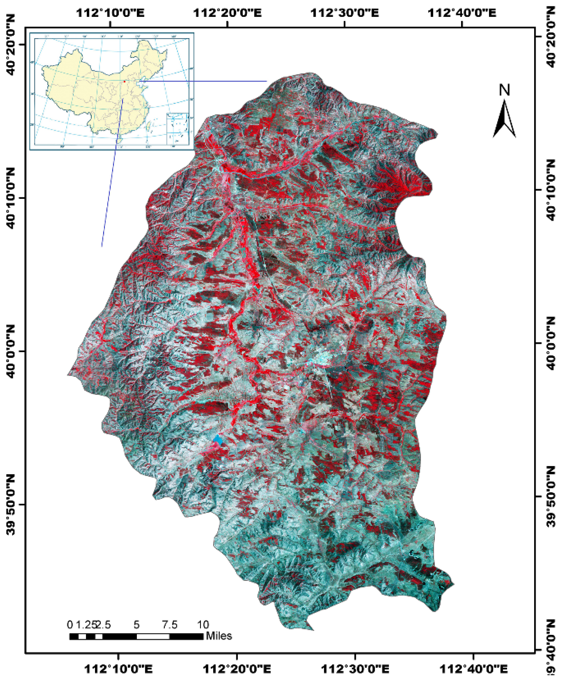
2.1. Study Area

The research was conducted for Youyu county in northwestern Shanxi province in China (Figure 1). Youyu county is part of the Three North Shelter Forest Program in China. With continuous afforestation and ecological constructions, Youyu has now become the “fortress oasis”. The forest cover of Youyu was only 0.3% before the 1950s, and the desertification area caused by soil erosion accounted for 76.2% of its total area. Residents of Youyu have started planting trees since the “Three North Shelter Forest Program” was initiated. After decades of unremitting afforestation efforts, Youyu’s forest coverage has increased substantially, and the ecological environment has been improved. Youyu, therefore, represents an ideal case for forest cover studies to evaluate the Three-North Shelter Forest Program.
Youyu county is located in the forefront of Mu Us Desert, and is surrounded by mountains from which flows the Cangtou River. In this region, the elevations are generally higher in the south than in the north. The county of Youyu reaches a north-south extent of 67.7 km and east-west width of 45.7 km, with a total area of 1967 square kilometers.
Youyu has a monsoon-influenced, semi-arid continental climate, with warm humid summers, and cold dry winters. The average elevation is about 1344 m. Due to its high elevation and dry winter climate, monthly average temperature ranges from −14.4 °C to 19.5 °C in January and July, respectively. The annual precipitation is 410 millimeters, three-fourths of which occurs from June through September.
Figure 1. Youyu county in Shanxi Province, China. The imagery represent a false-color composite of one Landsat image acquired on 10 July 2009.
Remotesensing 08 00062 g001

2.2. Data Collection and Preprocessing

2.2.1. Airborne LiDAR Data

Airborne LiDAR data were acquired during 19 to 28 September in 2009 with a Leica ALS60 laser system at an altitude of approximately 1000 m. The system was equipped with Multiple Pulses in Air (MPiA) technique, such that high density data can be obtained when flying at a high altitude.
The lateral overlaps of flight lines were set at least 5% on each side. The LiDAR sensor operated at a wavelength of 1064 nm. The recorded data have a nominal pulse spacing of 1.45 m and a point density of 0.46 pulses per m2. Up to four returns per pulse were recorded.

2.2.2. Landsat TM and ETM+ Imagery

Our study area is covered by one Landsat path 34 row 32. We downloaded the Landsat time-series stacks between 1986 and 2013 over the study region from the United States Geological Survey (USGS) data archive, as is shown in Table 1. The downloaded data are terrain corrected as level 1T (L1T) products. Radiometric calibration and atmospheric correction were performed and the surface reflectance were acquired with Landsat Ecosystem Disturbance Adaptive Processing System (LEDAPS) [16].
To screen clouds and cloud shadows, we preprocessed the Landsat imagery using the FMASK algorithm [17]. To reduce the influences of vegetation phenology and illumination geometry on surface spectral reflectance, only images acquired during the growing season (defined as early May to late September) were used in analysis. There may still exist some phenology difference within these days, it will be further reduced with Landtrendr algorithm [8], details can be find in Section 3.2.2. There are no cloud-free images available for the years of 1988, 1991, 1992, 1996, and 1997. To ensure a high level of co-register accuracy, LiDAR data was co-registered with Landsat image in 2009. We selected 35 ground control points and performed a second-order polynomial transformation and nearest neighbor resampling. Results showed a root mean square error (RMSE) of 0.63 m.
Table 1. Landsat imagery information.
YearJulian DayDay/MonthYearJulian DayDay/Month
19861599 June200319010 July
198725816 September200424129 August
198919919 July 16110 June
2154 August20052519 September
199013819 May 1877 July
23423 August200616616 June
199325816 September20071533 June
19941811 July20082441 September
199526422 September 26017 September
19981811 July200919010 July
199926725 September201019313 July
200020625 July201122817 August
1821 July201223927 August
20011522 June201317727 June
200223524 August 25715 September

2.2.3. Field Experiment Data
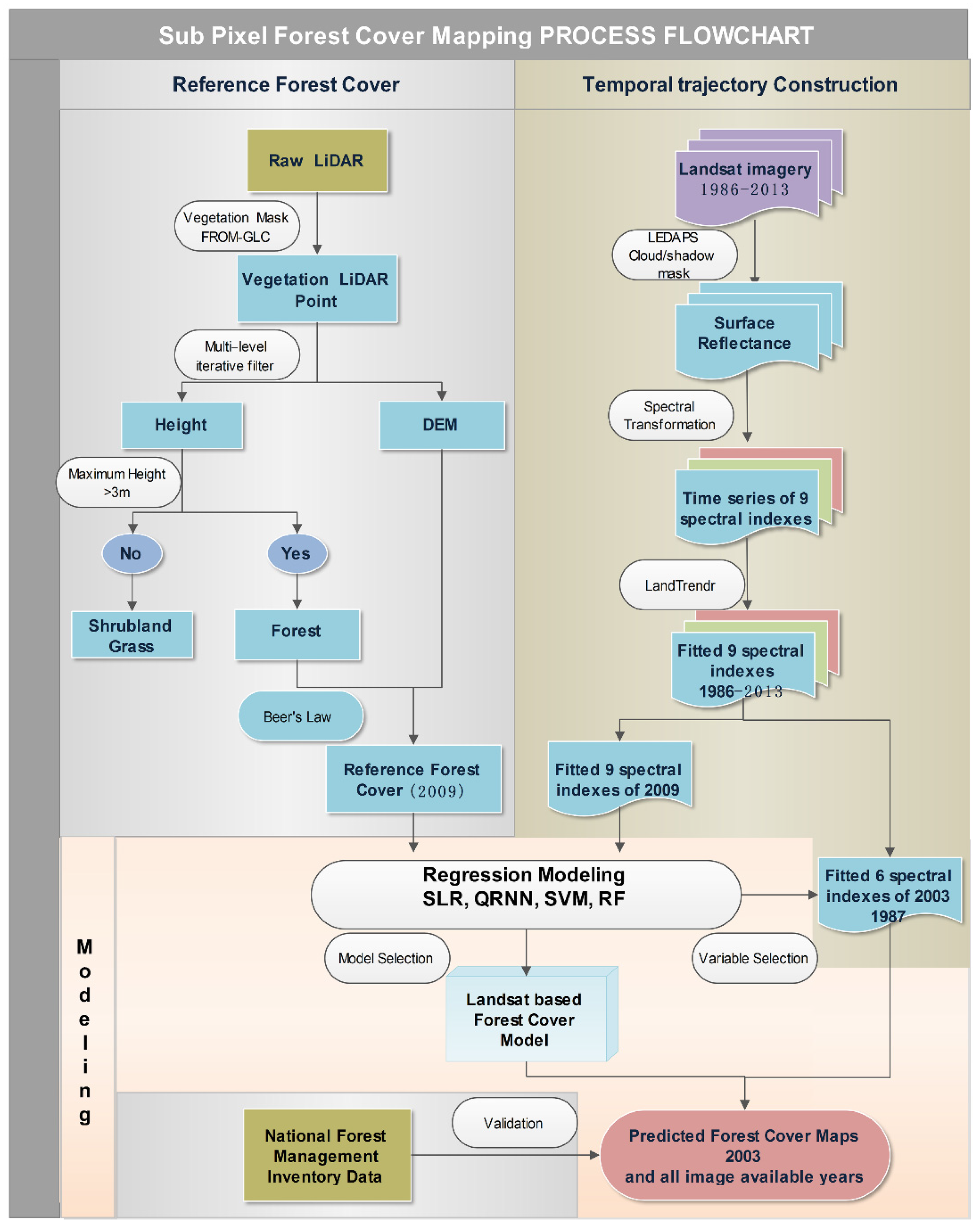
The field experiment was carried out in 78 plots, each plot with the size of 30 m × 30 m. To reduce the location error, the location of each plot was determined according to the pixel center location of Landsat image in 2003. Within each plot tree stands share similar structure, and differentiate from its neighborhood plots. The sampling is designed to avoid spatial autocorrelation. The coverage of each plot was surveyed during 2003–2004 by line intercepts method [18], with an interval of 1 m, and only counted tree heights greater than 3 m.

3. Method

Our approach mainly includes four steps. The first step involves extracting the referenced sub-pixel forest cover from LiDAR data. By “sub-pixel forest cover”, we refer to evaluating the percentage of forest within each 30 m resolution Landsat pixel. The second step builds the trajectory Landsat spectral data with the Landtrendr noise reduction and fitting method. The third step is to build the statistical relationships between sub-pixel forest cover and Landtrendr fitted spectral data, as well as original Landsat spectral data. Lastly, we predict forest cover for other years using the derived models. The process flowchart was represented in Figure 2. Four steps were shown in different background.

3.1. Extracting Reference Forest Cover

Sub-pixel forest cover in 2009 was extracted from LiDAR as the reference for forest cover evaluation over time. Since a high accuracy forest cover dataset could lay a better foundation for subsequent modeling, our strategy is to identify the forest area according to land cover dataset and maximum height, and then calculate the forest cover with a Beer’s Law modified model [19].
Non-vegetated areas, including impervious, water, and agriculture areas, were masked out from the raw LiDAR point cloud with a 30 m resolution global land cover dataset named Finer Resolution Observation and Monitoring-Global Land Cover (FROM-GLC) [19]. FROM-GLC that covers our study area was built based on Landsat TM imagery of 2009. The classification results in terms of vegetation and non-vegetation areas were considered satisfactory in our visual inspection of Landsat imagery.
Since this study was designed to detect forest cover change, we excluded areas occupied by short vegetation such as shrub and grass. Following previous studies, forests are defined as area with tree heights greater than 3 meter [20]. To derive the digital elevation model (DEM) and canopy height model (CHM), the raw LiDAR point cloud was processed with RiSCAN PRO 2.0 software package (Riegl GmbH, Horn, Austria), which incorporated a multi-level iterative terrain filter [21]. If the maximum height within a Landsat pixel is less than 3 m, we consider the pixel is dominated by short vegetation and exclude the corresponding Landsat pixel for analysis. DEM data would also assist to further separate the canopy and below-canopy LiDAR point cloud.
Figure 2. Flowchart for the sub-pixel forest cover process.
Remotesensing 08 00062 g002
For the forested area, forest cover (FC) can be calculated by dividing the number of returns above a height threshold (h) by the total number of returns for each Landsat pixel within a 30-m resolution. In this research, we adopted a derivative model [19] based on Beer’s law to extract forest cover reference in 2009. The potential two-way transmission loss of pulse energy was taken into account for intermediate or last returns in this LiDAR-based model. This model is less sensitive to sensor pulse repetition frequency and canopy height and, as a result, the least amount of calibration was required when applied to large areas with varied forest types. The model has shown to provide accurate forest cover as a basis for further analysis. In this model, the forest cover can be expressed as follows:
F C = I h I T o t a l = 1 I G r o u n d I T o t a l =   1 ( ( I G r o u n d S i n g l e I T o t a l ) + I G r o u n d L a s t I T o t a l ( I F i r s t + I S i n g l e I T o t a l ) + I I n t e r m e d i a t e +   I L a s t I T o t a l )
In the equation above, I G r o u n d represented the sum of all intensity below canopy, which was determined by the canopy height threshold (see below). I T o t a l was the intensity of all returns including single, first, intermediate, and last returns. The calculated reference forest cover in 2009 was shown in result Section 4.1. In agreement with the global definition of forest, pixels with forest cover exceeding ten percent were reserved [22].
A height threshold was involved in the model to separate the ground and canopy point. This model parameter could vary with forest type and local forest condition. Ahmed and Smith employed 1.50 m and found that the results performed reasonably well [16,23]. In this study, we defined the threshold by the transition zone between the forest over-story and under-story where the least number of LiDAR returns were detected. We counted the number of returns in each vertical layer using voxel statistics with an interval of 0.1 m, and determined the appropriate threshold as 1.4 m, details can be found in supplementary Figure S1.
A stratified sampling [24] was applied to the referenced data to diminish the uncertainty of the training sample and auto-correlation. The dataset was ordered according to descending forest cover values and was split into 20% percentiles. We randomly selected half of the sample within each percentile.

3.2. Temporal Trajectory Construction

3.2.1. Spectral Indexes Extraction for the Time-Series Trajectory

A suite of spectral indexes were extracted from Landsat time-series imagery between 1986 and 2013. Each spectral index was used to build temporal trajectories for each Landsat pixel and construct empirical models with sub-pixel forest cover from LiDAR data.
We used four vegetation indexes: Normalized Difference Water Index (NDWI) [25], Normalized Burn Ratio (NBR), Normalized Difference Vegetation Index (NDVI), and Enhanced Vegetation Index (EVI). NDWI has been interpreted as an indicator of changes in water content of plant canopies, and has been used to detect forest changes [26]. NBR represents the vegetation condition and is sensitive to forest disturbance [27]. NDVI is a widely used measure of live green vegetation, and EVI complements NDVI in vegetation studies by improving the ability of forest change detection [28].
We also used five indexes based on the tasseled-cap transformation [29]: tasseled cap brightness (TCB), greenness (TCG), wetness (TCW), tasseled cap distance (TCD), and tasseled cap angle (TCA). As the names indicated, TCB, TCG, and TCW contain significant information for background reflectance, green vegetation, and wetness. TCD describes vegetation structure and composition. TCA is related to the proportion of vegetation cover within a Landsat pixel [30].

3.2.2. Temporal Fitting of Spectral Indexes Trajectories

The forest cover time-series trajectories mainly depend on its history (plantation, disturbance, and recovery). So, for each spectral index described above, we took temporal factors into account and processed the time-series trajectories with LandTrendr, a temporal segmentation and smoothing algorithm developed by Kennedy [27]. By reducing the inter-annual noise introduced by atmospheric condition, solar angle, phenology, and imperfection in geometric registration and radiometric calibration, LandTrendr was able to capture the short-term changes and maintain the long-term trends related to disturbance and recovery. As a result, the algorithm outperformed the single-date evaluation [31] or two-date change assessment [30,32] in previous studies, and could improve forest cover estimation at any given point along the temporal trajectory and enhance the forest cover change detection capability.
The spectral trajectory for each forest pixel was identified as a series of sequential straight-line segments. LandTrendr algorithm removed singular value according to the consistency before and after the singular value year, and extracted up to six straight-line segments to simplify the temporal trajectory of the Landsat time series at each pixel location. Then a fitting algorithm was applied to each segment, not only to minimize the noise coming from those aforementioned factors, but also capture the changes during all the time periods.
Briefly, the LandTrendr algorithm identified the time-series spectral trajectory as a series of sequential lines. As a result, a stack of near yearly-fitted spectral index images were obtained, and those spectral values directly taken from the fitted line were put into the forest cover estimation model as predictors. Since the first or the last year lacks part of the neighborhood information, it was difficult to detect the singular value. Therefore, we only detected forest cover change from 1987 to 2012, and neglected information from 1986 (the first year) and 2013 (the last year).

3.3. Forest Cover Modeling

We compared the result using original Landsat spectral indexes and temporal trajectory fitted spectral indexes with four types of forest cover statistic modeling algorithms. The used modeling algorithms include a stepwise linear regression (SLR) model and three machine-learning algorithms, including quantile regression neural network (QRNN), support vector machine (SVM), and regression tree random forest (RF).
SLR builds the multiple linear regressions between sub-pixel forest cover and Landsat spectral indexes iteratively using a stepwise method. For each iteration, the model is improved by adding the independent variable with the most predictive power and removing the insignificant independent variables. SLR has been used in a variety applications such as biomass estimation and wetland inundation mapping [33,34].
QRNN is the analog of linear quantile regression in the field of artificial neural network. The model uses a finite smoothing algorithm and searches for the optional left censoring, which is suitable for mixed discrete-continuous prediction (such as precipitation). The number of hidden nodes was set to four, and the hidden layer transfer function was defined as sigmoid to get the nonlinear model.
SVM attempts to determine a hyperactive plane to implement the structural risk minimization. We utilized the radial basis function (RBF) kernel with the C-SVM classifier in “caret” provided in R [35]. The particle swarm optimization (PSO) method was adopted to select the parameters. γ is the kernel parameter which defines the influence of a single training example and is set in the range of 0.01–1000. stands for the parameter for the marginal cost function, and was set in the range of 0.25–1024. All variables were scaled from −1 to 1 to speed up convergence of the regression and improve the estimation accuracy.
RF has shown good performance in vegetation height mapping [36], land cover mapping [37,38,39], and biomass estimation [40]. In construction of the regression trees, random forest utilized different bootstrap samples of data and changed how the regression trees are constructed as well. The node of trees is split by randomly choosing the subset of forest cover predictors and selecting the best of these. The RF algorithm is robust against over fitting and performs well relative to other classifiers [41]. Two parameters need to be settled including numFeatures, which means the number of features to be randomly selected at each node, and numTrees that means number of trees generated. We employ the suggested value of numFeatures as one third of number of features, and the numTrees was set to 500 considering the limitation of computer memory [36].
Although RF and SVM is naturally resistant to non-informative predictors, non-informative predictors can negatively affect some models [42]. We checked the importance of each variables as mean decrease in accuracy with the out of bag (OOB) samples [43]. All four methods represent similar patterns, and most of the variables play a relatively important role in each model, details can be found in the supplementary Figure S2. Then, for each regression method, the backward elimination approach was adopted, and the least important variable was thrown out until the out-of-bag prediction accuracy dropped [44]. Six out of nine variables were chosen. EVI, TCD, and TCW were discarded in further analysis.

3.4. Validation and Uncertainty Analysis

The k-fold and leave-one-out cross-validations were utilized to estimate the uncertainty of forest cover models.
The uncertainty of forest cover evaluation induced by uncertainty in predictors and model structure could be obtained from whole number of prediction with finite samples and estimated by the standard deviation of the k-fold cross-validation. In this study, ten-fold cross-validation was used. In addition, we randomly selected 5% of the entire sample as validation sample to evaluate the performance of forest cover model with scatter plots.
To assess if the forest cover model built with 2009 data was applicable to other years, the model was directly applied to the fitted Landsat spectral indexes for 2003 (as described in Section 3.2). Results were then evaluated with the Forest Management Inventory Data.
The performance of those regression models was evaluated in accordance with R 2 , root mean square error (RMSEs), and mean error (ME). The optimal regression model with the lowest RMSE was employed to predict forest cover for all available years of data.

4. Results and Discussion

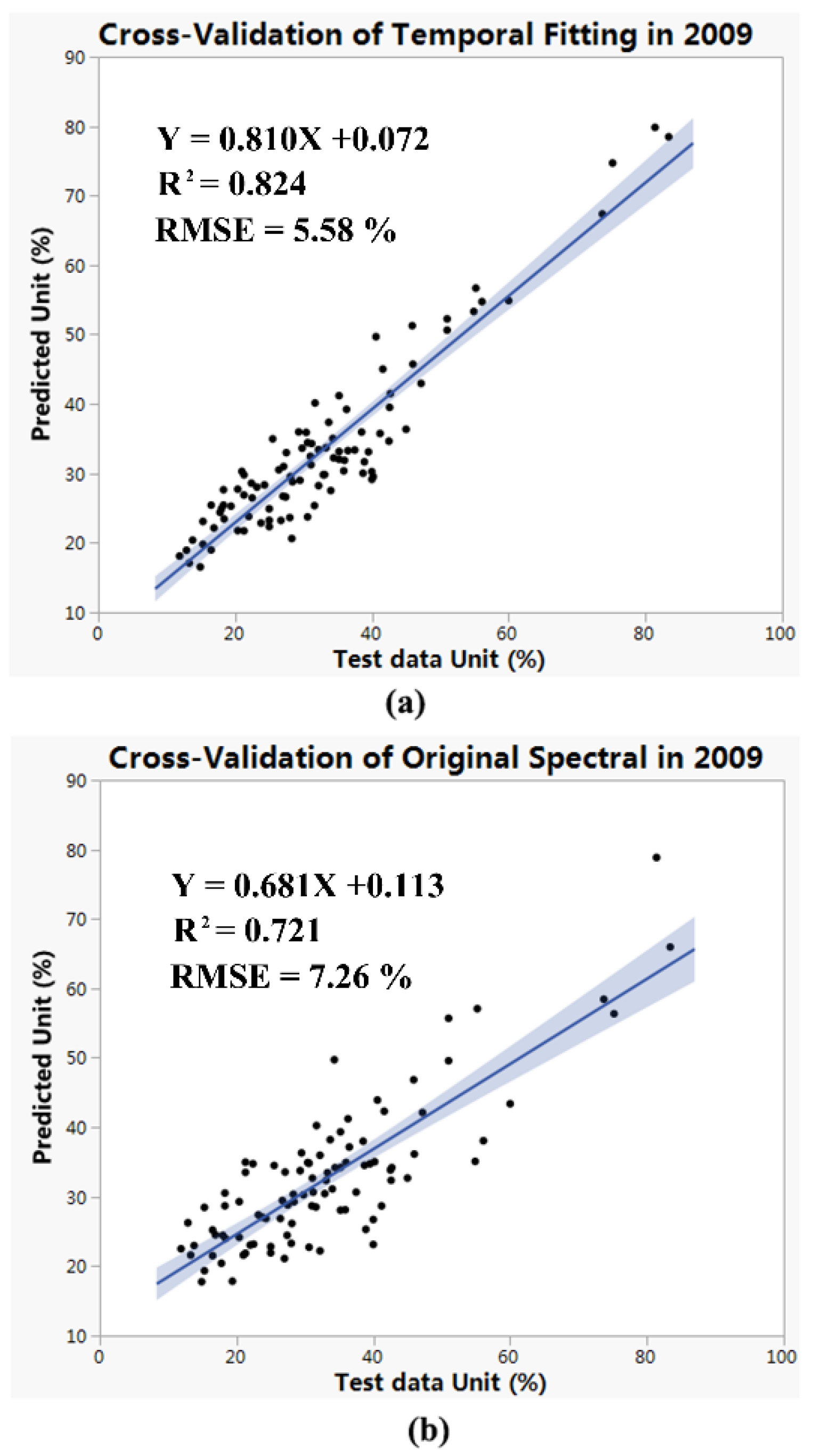
4.1. Performance of Forest Cover Regression Models in 2009

The sub-pixel forest cover for the LiDAR measured year in 2009 were shown in Figure 3. The result were extracted from airborne LiDAR data using the Beer’s Law modified method. Non-vegetation area masked from FROM-GLC dataset were shown in white.
Figure 3. Sub-pixel forest cover estimated from airborne LiDAR data in 2009.
Remotesensing 08 00062 g003
Four forest cover regression models were evaluated according to the R 2 , RMSE and ME in Table 2. We compared the result with original spectral indexes (O) and temporal trajectory fitting (F).
Notably, predictors with time-series processing outperform the original spectral indexes for each regression model in varying degrees.
As can be seen from the comparison of modeling results in Table 2, the SLR model performed poor with R 2 of 0.59. SLR assumes a global linear relationship between the spectral indexes and forest cover, which may not be suitable for forest cover modeling. The use of non-linear regression may be more appropriate.
Although QRNN did not perform as well as expected in terms of its R 2 value (0.65), the model achieved a relatively low RMSE of 7.84. We assume that the result is due to the lack of efficient tuning for better model parameters.
Table 2. Modeling comparison with different algorithm in 2009. The comparison was performed with original spectral indexes (O) and temporal trajectory (T), separately. SD stands for standard derivation. The best results were marked in bold.
Results with Ten-Fold Cross-Validation
R2RMSESD_R2SD_RMSEME
SLRO0.509.290.0340.34−0.006
T0.598.480.0270.17−0.002
QRNNO0.548.750.0330.29−0.021
T0.657.840.0220.29−0.042
SVMO0.687.470.0340.37−0.746
T0.736.080.0240.32−0.486
RFO0.727.260.0260.320.033
T0.825.190.0150.20−0.010
With respect to the SVM method, it achieved acceptable RMSE and R 2 values, but its standard deviation and ME values were the greatest among the four methods.
Random forest, on the other hand, generated well-predicted forest cover in terms of both RMSE and R 2 values. RF regression has the ability to recognize complex non-parametric relationships. As a result, random forest is robust to the shortage of reference data. Furthermore, the impact caused by the distribution and uncertainty of training sample would be reduced because of its bootstrapping strategy [34].
Based on the ten-fold cross validation results, we further investigated the performance of RF through scatter plots in Figure 4. To show the distribution of validation data, we set aside five percent of the random sample to use as a training set. The validation was performed 10 times. The regression line revealed that the predicted results fit well with the cover calculated from LiDAR data.
Compared to the time-series fitted model in Figure 4, the RF model based on single-date Landsat data (Figure 4b) performed relatively well with an R 2 = 0.72 ± 0.026 and R M S E = 7.26 % ± 0.320 % . Including the temporal trajectory fitting process (Figure 4a) for the RF model substantially improved the overall performance ( R 2 = 0.82 ± 0.015 and R M S E = 5.19 % ± 0.204 % ). The fitted spectral indexes incorporating the historic information infuse the model with better prediction power and yield better results of lower bias and higher correlation, which was confirmed by Powell et al. [30] and Sulla-Menashe et al. [45]. The uncertainty assessed by standard derivation of the ten-fold cross-validation, indicates that the uncertainty of the original spectral indexes is larger by one-third than with the temporal trajectory fitting approach. The scatterplots revealed an improvement in the prediction particularly in the high and low forest cover range, increasing the dynamic range of the predictions.
Compared with a global, Landsat-based tree cover dataset [17] produced by rescaling of MODIS VCF with a piecewise linear function, our result performed well for high forest cover range. The rescaling result retained the saturation artifact of the MODIS VCF at greater than or equal to 80% tree cover, and shown negative bias at high cover [46]. Since no LiDAR data available to calibrate result in China, the rescaling result appears problematic when checked at the local scale, with the maximum forest cover of 29% in 2000 for our study area.
Figure 4. Scatter plots of predicted forest cover against LiDAR data results. (a) Validation of forest cover with temporal trajectory fitting algorithm; (b) validation of forest cover with original spectral indices. The blue area represents the 95% confidence intervals for the regression line.
Remotesensing 08 00062 g004

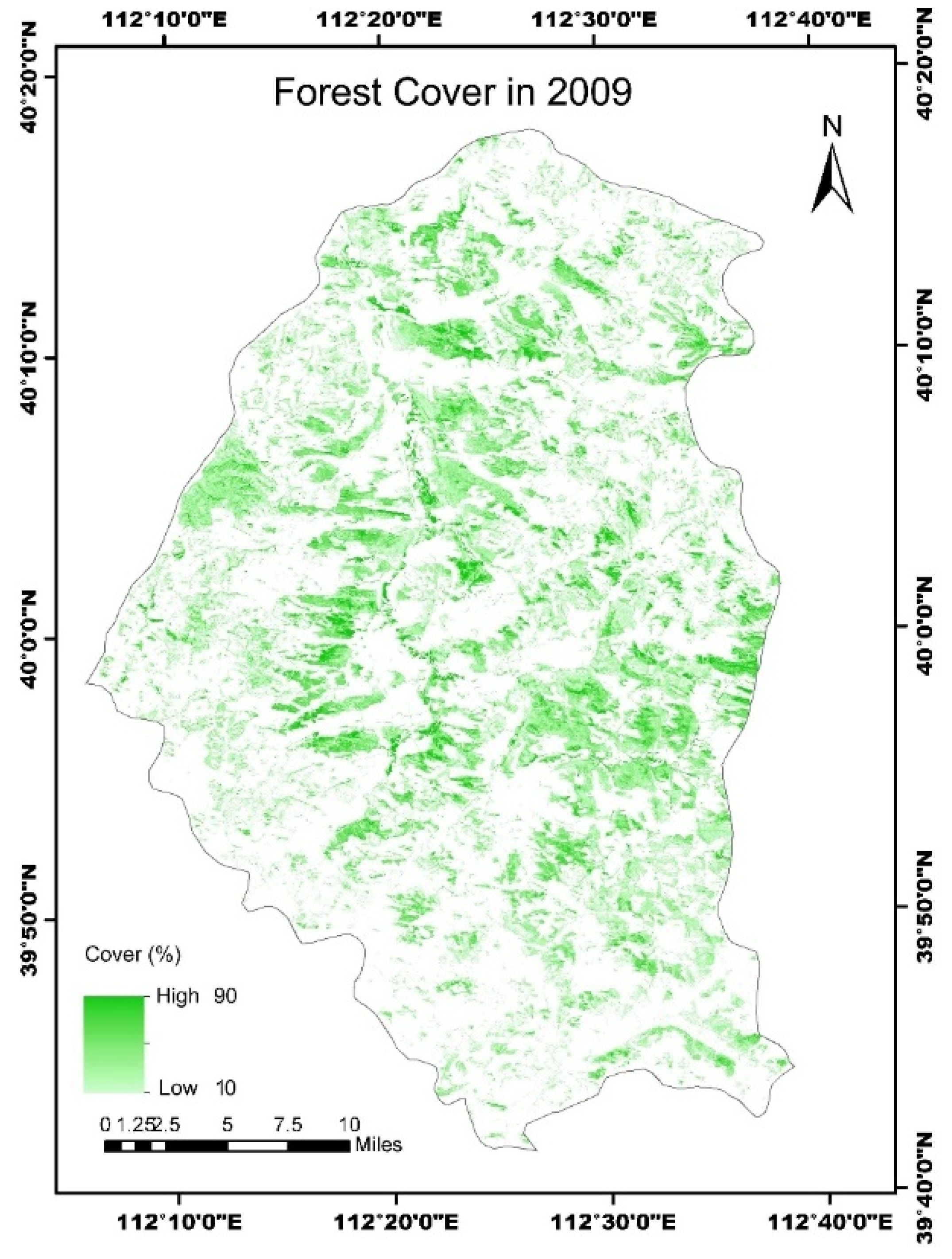
4.2. Performance of Trajectory Landsat Imagery in Forest Cover Mapping

With respect to modeling algorithms, RF with temporal-trajectory fitted spectral indexes performs the best in terms of coefficient of determination ( R 2 ) and prediction errors (RMSE), and RF was chosen to predict the forest cover for all Landsat imagery available each year.
The results in Figure 5 shown that the forest cover model predict forest cover along the temporal trajectory effectively. By coupling LiDAR analysis with Landsat spectral indices, this allowed us to estimate crown closure over time. In the following discussion, this model was applied to all available years to extract time-series forest cover condition and forest cover change.
Figure 5. Scatterplot of predicted forest cover against field data in 2003.
Remotesensing 08 00062 g005

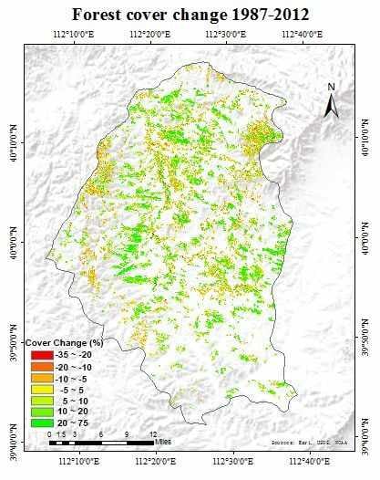
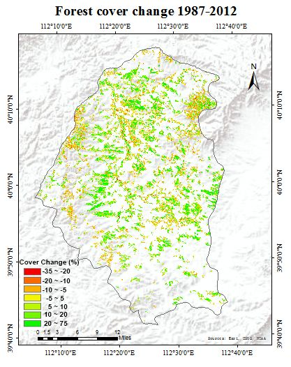
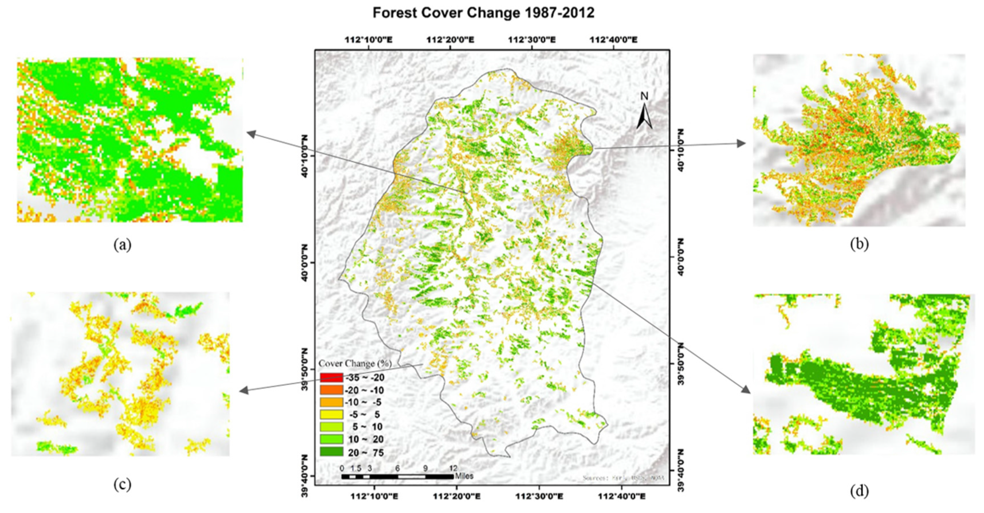
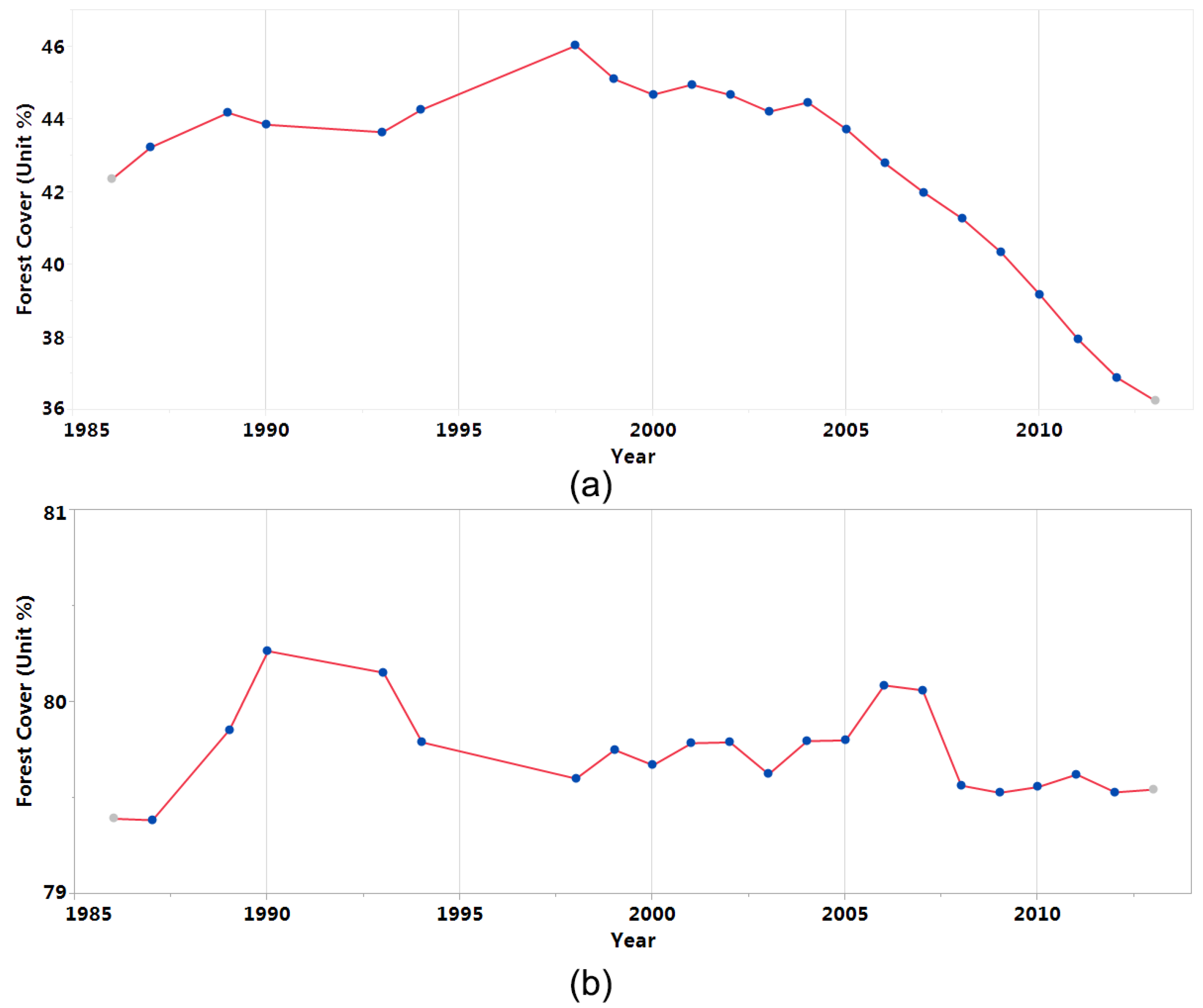
4.3. Forest Cover Change

Forest cover changes were obtained from 1987 to 2012 as shown in Figure 6. Extrapolating to the county-level, the average forest cover represents a significant increase from the 1987 estimate of 15.5% to the 2012 estimate of 37.8%, under the combined change of natural forest and plantation. This finding agrees well with the results of Liu and Gong [47].
The plantation and native forest area were separated with visual inspection of high-resolution images in Google Earth. The plantation area represents a regular pattern while native forest is naturally spread and not thickened, which shows natural and irregular pattern. The plantation was mainly implemented in the center of Youyu county along the Cangtou River, thus largely promoting the accumulation of forest cover. As can be seen from Figure 6a,d, forest cover in these plantation areas increases dramatically. Nonetheless, forest cover in the southwest area (shown in Figure 6c) stays the same, and tree crown does not show significant growth.
Figure 6. Forest cover change from 1987 to 2012. (a) Plantation area with forest cover increases; (b) native forest; (c) plantation area with unchanged forest cover; and (d) plantation area.
Remotesensing 08 00062 g006
The native forest represents different pattern was shown in Figure 6b, the difference is probably due to various water-heat combinations [48].
We then examined successive forest cover trends across the time series, revealing the status and change along the time. As can be seen from Figure 7 and Figure 8, forest cover during the designated period revealed different trends.
Figure 7. Annual forest cover condition and dynamic for plantation area.
Remotesensing 08 00062 g007
For the plantation area shown in Figure 6d, forest cover was on a constant rise as illustrated in Figure 7. The dynamics of forest cover over time resembles a logistic (S-shaped) growth curve, which agree with the results of managed forest by Dewar and Roderick [49]. After 20 years of growth, the growth rate slows down when resources are limited, and forest cover reaches a stable level. This growth period is roughly consistent with the local response to the national policy of “Three North Shelter Forest Program” for Shanxi Province. For mature forest, with the stand age of 20 to 30 years for aspen [50], additional research is suggested on the mortality of trees for the next 5 to 10 years and the corresponding strategy to deal with the anticipated mortality, as in investigated by Esseen et al. [51], and Monserud [52] for the old-growth forest.
For the native forest area shown in Figure 6b, various patterns could be detected. This is area where crown cover is being established. Figure 8a,b, represent two different patterns of forest cover—decreasing or fluctuating. For the cover loss area, there is a slow increase before 1998, which gradually drops afterwards. Although a decease was detected, it remains relatively high in coverage. For the area whose crown cover fluctuates, additional research is suggested on the driving factor for the variation in forest cover, as is presented by Crowther et al. [53].
Figure 8. Forest cover dynamic for native forest area from 1987 to 2012. (a) Decrease; and (b) fluctuation.
Remotesensing 08 00062 g008

4.4. Limitations

In many areas of China, there was a lack of Landsat imagery in the 1990s. In addition to the Landsat 7 ETM+ gaps caused by the failure of the Scan Line Corrector (SLC), cloud and its shadow make it even harder to obtain sufficient images for each year. Adding the Landsat MSS dataset would also be helpful to lengthen the temporal detection period, while the comparability introduced by system-inherent differences should be further examined.
As can be seen from Figure 7, plantation follows a logistic S-shaped curve. The logistic curve can be approximated fairly well by several straight-line segments. However, there is still room for improvement in fitting the model and in automatic parameter selection. A series of piecewise logistic functions can be used to represent intra-annual vegetation dynamics, as the previous study applied to MODIS time series data [54]. When applied to global scale, a method should be processed without setting thresholds or empirical constants [55].
The sampling strategy would violation of independence of the data [16], and sample size would influence the regression result [40]. More efforts should focused on the design of sampling.

5. Conclusions

Deriving historical and up-to-date forest cover information is important for forest management and monitoring. In this research, we developed a new approach to map time-series sub-pixel forest cover with Landsat and LiDAR data, and we further evaluated this method for deriving change information in forest cover in the Northeastern China county of Youyu.
Our results show that the inclusion of the Landtrendr temporal trajectory fitting process considerably increased the model performance versus the original spectral indices with better results of lower bias and higher correlation. In comparing regression methods, we found that random forest outperformed the SVM, NN, and SLR in quantitative forest cover estimation. A random forest model incorporating temporal trajectory fitting yields the best agreement with validation data ( R 2 = 0.82 and R M S E = 5.19 % ).
Our results revealed that forest cover rose from 15.5% in 1987 to 37.8% in 2012—an increase by 144.1%. Accordingly, the “Three North Shelter Forest Program” obtained impressive achievements with their afforestation program in this arid region.
More focused research is suggested to explore better sigmoid curve fitting along the time-series trajectories, aimed at better depicting forest status. Furthermore, future research should focus on the climate response to forest plantation and forest change over long periods of time, especially the mortality of trees and corresponding management planning.

Supplementary Files

Supplementary File 1

Acknowledgments

This research was partially supported by Special Fund for Meteorology Scientific Research in the Public Welfare (GYHY201506010), Youth Innovation Promotion Association CAS, National Natural Science Foundation of China (Grant No. 41401484), and China Scholarship Council (Project reference number 201404910437). The authors also acknowledge the valuable discussions with Robert A. Monserud at Rocky Mountain and Pacific Northwest Research Stations, USDA Forest Service. We would also like to thank three anonymous reviewers for insightful comments and improvements to the manuscript.

Author Contributions

All authors have made significant contributions to the manuscript. Xiaoyi Wang, Huabing Huang and Peng Gong conceived and designed the experiments; Xiaoyi Wang and Huabing Huang performed the experiments; Xiaoyi Wang and Gregory S. Biging analyzed the data; Qinchuan Xin , Yanlei Chen, Jun Yang and Caixia Liu contributed in manuscript revision. Gregory S. Biging and Peng Gong contributed in the language editing.

Conflicts of Interest

The authors declare no conflict of interest.

References

  1. Bonan, G.B. Forests and climate change: Forcings, feedbacks, and the climate benefits of forests. Science 2008, 320, 1444–1449. [Google Scholar] [CrossRef] [PubMed]
  2. Pan, Y.; Birdsey, R.A.; Fang, J.; Houghton, R.; Kauppi, P.E.; Kurz, W.A.; Phillips, O.L.; Shvidenko, A.; Lewis, S.L.; Canadell, J.G. A large and persistent carbon sink in the world’s forests. Science 2011, 333, 988–993. [Google Scholar] [CrossRef] [PubMed]
  3. Hansen, M.C.; Potapov, P.V.; Moore, R.; Hancher, M.; Turubanova, S.; Tyukavina, A.; Thau, D.; Stehman, S.; Goetz, S.; Loveland, T. High-resolution global maps of 21st-century forest cover change. Science 2013, 342, 850–853. [Google Scholar] [CrossRef] [PubMed]
  4. Yang, J.; Gong, P.; Fu, R.; Zhang, M.; Chen, J.; Liang, S.; Xu, B.; Shi, J.; Dickinson, R. The role of satellite remote sensing in climate change studies. Nat. Clim. Chang. 2013, 3, 875–883. [Google Scholar] [CrossRef]
  5. Tokola, T.; Löfman, S.; Erkkilä, A. Relative calibration of multitemporal landsat data for forest cover change detection. Remote Sens. Environ. 1999, 68, 1–11. [Google Scholar] [CrossRef]
  6. Townshend, J.R.; Masek, J.G.; Huang, C.; Vermote, E.F.; Gao, F.; Channan, S.; Sexton, J.O.; Feng, M.; Narasimhan, R.; Kim, D. Global characterization and monitoring of forest cover using Landsat data: Opportunities and challenges. Int. J. Digit. Earth 2012, 5, 373–397. [Google Scholar] [CrossRef]
  7. Schroeder, T.A.; Cohen, W.B.; Yang, Z. Patterns of forest regrowth following clearcutting in western oregon as determined from a Landsat time-series. For. Ecol. Manag. 2007, 243, 259–273. [Google Scholar] [CrossRef]
  8. Kennedy, R.E.; Yang, Z.; Cohen, W.B.; Pfaff, E.; Braaten, J.; Nelson, P. Spatial and temporal patterns of forest disturbance and regrowth within the area of the northwest forest plan. Remote Sens. Environ. 2012, 122, 117–133. [Google Scholar] [CrossRef]
  9. Wang, X.; Huang, H.; Gong, P.; Liu, C.; Li, C.; Li, W. Forest canopy height extraction in rugged areas with ICESAT/GLAS data. IEEE Trans. Geosci. Remote Sens. 2014, 52, 4650–4657. [Google Scholar] [CrossRef]
  10. Asner, G.P.; Mascaro, J.; Muller-Landau, H.C.; Vieilledent, G.; Vaudry, R.; Rasamoelina, M.; Hall, J.S.; van Breugel, M. A universal airborne Lidar approach for tropical forest carbon mapping. Oecologia 2012, 168, 1147–1160. [Google Scholar] [CrossRef] [PubMed]
  11. Chen, Q. Retrieving vegetation height of forests and woodlands over mountainous areas in the pacific coast region using satellite laser altimetry. Remote Sens. Environ. 2010, 114, 1610–1627. [Google Scholar] [CrossRef]
  12. Huang, H.; Gong, P.; Cheng, X.; Clinton, N.; Li, Z. Improving measurement of forest structural parameters by co-registering of high resolution aerial imagery and low density Lidar data. Sensors 2009, 9, 1541–1558. [Google Scholar] [CrossRef] [PubMed]
  13. Liu, C.; Huang, H.; Gong, P.; Wang, X.; Wang, J.; Li, W.; Li, C.; Li, Z. Joint use of ICESAT/GLAS and Landsat data in land cover classification: A case study in Henan province, China. IEEE J. Sel. Top. Appl. Earth Obs. Remote Sens. 2015, 8, 511–522. [Google Scholar] [CrossRef]
  14. Huang, H.; Liu, C.; Wang, X.; Biging, G.S.; Yang, J.; Gong, P. Mapping vegetation heights in China with remotely sensed data. ISPRS J. Photogram. Remote Sens. 2016. Submitted. [Google Scholar]
  15. Chen, X.; Vierling, L.; Rowell, E.; DeFelice, T. Using Lidar and effective LAI data to evaluate Ikonos and Landsat 7 ETM+ vegetation cover estimates in a ponderosa pine forest. Remote Sens. Environ. 2004, 91, 14–26. [Google Scholar] [CrossRef]
  16. Ahmed, O.S.; Franklin, S.E.; Wulder, M.A. Integration of Lidar and Landsat data to estimate forest canopy cover in coastal British Columbia. Photogram. Eng. Remote Sens. 2014, 80, 953–961. [Google Scholar] [CrossRef]
  17. Sexton, J.O.; Song, X.-P.; Feng, M.; Noojipady, P.; Anand, A.; Huang, C.; Kim, D.-H.; Collins, K.M.; Channan, S.; DiMiceli, C. Global, 30-m resolution continuous fields of tree cover: Landsat-based rescaling of MODIS vegetation continuous fields with Lidar-based estimates of error. Int. J. Digit. Earth 2013, 6, 427–448. [Google Scholar] [CrossRef]
  18. Zhou, Q.; Robson, M.; Pilesjo, P. On the ground estimation of vegetation cover in australian rangelands. Int. J. Remote Sens. 1998, 19, 1815–1820. [Google Scholar] [CrossRef]
  19. Hopkinson, C.; Chasmer, L. Testing Lidar models of fractional cover across multiple forest ecozones. Remote Sens. Environ. 2009, 113, 275–288. [Google Scholar] [CrossRef]
  20. Koeln, G.T.; Jones, T.; Melican, J. Geocover Lc: Generating Global Land Cover from 7600 Frames of Landsat TM Data. In Proceedings of the ASPRS 2000 Annual Conference, Washington, DC, USA, 21–26 May 2000.
  21. Véga, C.; Durrieu, S. Multi-level filtering segmentation to measure individual tree parameters based on Lidar data: Application to a mountainous forest with heterogeneous stands. Int. J. Appl. Earth Obs. Geoinf. 2011, 13, 646–656. [Google Scholar] [CrossRef] [Green Version]
  22. FAO. Global Forest Resources Assessment 2000: Main Report; Food and Agriculture Organization of the United Nations: Rome, Italy, 2000. [Google Scholar]
  23. Smith, A.; Falkowski, M.J.; Hudak, A.T.; Evans, J.S.; Robinson, A.P.; Steele, C.M. A cross-comparison of field, spectral, and Lidar estimates of forest canopy cover. Can. J. Remote Sens. 2009, 35, 447–459. [Google Scholar] [CrossRef]
  24. Trost, J.E. Statistically nonrepresentative stratified sampling: A sampling technique for qualitative studies. Qual. Sociol. 1986, 9, 54–57. [Google Scholar] [CrossRef]
  25. Gao, B.-C. NDWI—A normalized difference water index for remote sensing of vegetation liquid water from space. Remote Sens. Environ. 1996, 58, 257–266. [Google Scholar] [CrossRef]
  26. Jin, S.M.; Sader, S.A. Comparison of time series tasseled cap wetness and the normalized difference moisture index in detecting forest disturbances. Remote Sens. Environ. 2005, 94, 364–372. [Google Scholar] [CrossRef]
  27. Kennedy, R.E.; Yang, Z.; Cohen, W.B. Detecting trends in forest disturbance and recovery using yearly landsat time series: 1. LandTrendr—Temporal segmentation algorithms. Remote Sens. Environ. 2010, 114, 2897–2910. [Google Scholar] [CrossRef]
  28. Huete, A.; Didan, K.; Miura, T.; Rodriguez, E.P.; Gao, X.; Ferreira, L.G. Overview of the radiometric and biophysical performance of the MODIS vegetation indices. Remote Sens. Environ. 2002, 83, 195–213. [Google Scholar] [CrossRef]
  29. Crist, E.P. A TM tasseled cap equivalent transformation for reflectance factor data. Remote Sens. Environ. 1985, 17, 301–306. [Google Scholar] [CrossRef]
  30. Powell, S.L.; Cohen, W.B.; Healey, S.P.; Kennedy, R.E.; Moisen, G.G.; Pierce, K.B.; Ohmann, J.L. Quantification of live aboveground forest biomass dynamics with Landsat time-series and field inventory data: A comparison of empirical modeling approaches. Remote Sens. Environ. 2010, 114, 1053–1068. [Google Scholar] [CrossRef]
  31. Liang, L.; Chen, Y.; Hawbaker, T.J.; Zhu, Z.; Gong, P. Mapping mountain pine beetle mortality through growth trend analysis of time-series Landsat data. Remote Sens. 2014, 6, 5696–5716. [Google Scholar] [CrossRef]
  32. Pflugmacher, D.; Cohen, W.B.; Kennedy, R.E.; Yang, Z. Using landsat-derived disturbance and recovery history and Lidar to map forest biomass dynamics. Remote Sens. Environ. 2014, 151, 124–137. [Google Scholar] [CrossRef]
  33. Zhang, Y.; Liang, S.; Sun, G. Forest biomass mapping of northeastern China using GLAS and MODIS data. IEEE J. Sel. Top. Appl. Earth Observ. Remote Sens. 2014, 7, 140–152. [Google Scholar] [CrossRef]
  34. Huang, C.; Peng, Y.; Lang, M.; Yeo, I.-Y.; McCarty, G. Wetland inundation mapping and change monitoring using Landsat and airborne Lidar data. Remote Sens. Environ. 2014, 141, 231–242. [Google Scholar] [CrossRef]
  35. Kuhn, M. Building predictive models in R using the caret package. J. Stat. Softw. 2008, 28, 1–26. [Google Scholar] [CrossRef]
  36. Simard, M.; Pinto, N.; Fisher, J.B.; Baccini, A. Mapping forest canopy height globally with spaceborne Lidar. J. Geophys.Res. Biogeosci 2011, 116, G04021. [Google Scholar] [CrossRef]
  37. Gong, P.; Wang, J.; Yu, L.; Zhao, Y.; Zhao, Y.; Liang, L.; Niu, Z.; Huang, X.; Fu, H.; Liu, S.; et al. Finer resolution observation and monitoring of global land cover: First mapping results with landsat TM and ETM+ data. Int. J. Remote Sens. 2013, 34, 2607–2654. [Google Scholar] [CrossRef]
  38. Hao, P.; Zhan, Y.; Wang, L.; Niu, Z.; Shakir, M. Feature selection of time series MODIS data for early crop classification using random forest: A case study in Kansas, USA. Remote Sens. 2015, 7, 5347–5369. [Google Scholar] [CrossRef]
  39. Hao, P.; Wang, L.; Niu, Z. Potential of multitemporal Gaofen-1 panchromatic/multispectral images for crop classification: Case study in Xinjiang uygur autonomous region, China. J. Appl. Remote Sens. 2015, 9. [Google Scholar] [CrossRef]
  40. Fassnacht, F.; Hartig, F.; Latifi, H.; Berger, C.; Hernández, J.; Corvalán, P.; Koch, B. Importance of sample size, data type and prediction method for remote sensing-based estimations of aboveground forest biomass. Remote Sens. Environ. 2014, 154, 102–114. [Google Scholar] [CrossRef]
  41. Fernández-Delgado, M.; Cernadas, E.; Barro, S.; Amorim, D. Do we need hundreds of classifiers to solve real world classification problems? J. Mach. Learn. Res. 2014, 15, 3133–3181. [Google Scholar]
  42. Ishwaran, H. Variable importance in binary regression trees and forests. Electron. J. Stat. 2007, 1, 519–537. [Google Scholar] [CrossRef]
  43. Breiman, L. Out-of-Bag Estimation; Technical Report; Citeseer: Berkeley, CA, USA, 1996. [Google Scholar]
  44. Díaz-Uriarte, R.; De Andres, S.A. Gene selection and classification of microarray data using random forest. BMC Bioinf. 2006, 7. [Google Scholar] [CrossRef]
  45. Sulla-Menashe, D.; Kennedy, R.E.; Yang, Z.; Braaten, J.; Krankina, O.N.; Friedl, M.A. Detecting forest disturbance in the Pacific northwest from MODIS time series using temporal segmentation. Remote Sens. Environ. 2014, 151, 114–123. [Google Scholar] [CrossRef]
  46. Alexander, C.; Bøcher, P.K.; Arge, L.; Svenning, J.-C. Regional-scale mapping of tree cover, height and main phenological tree types using airborne laser scanning data. Remote Sens. Environ. 2014, 147, 156–172. [Google Scholar] [CrossRef]
  47. Liu, S.; Gong, P. Change of surface cover greenness in China between 2000 and 2010. Chin. Sci. Bull. 2012, 57, 2835–2845. [Google Scholar] [CrossRef]
  48. Niinemets, Ü. Responses of forest trees to single and multiple environmental stresses from seedlings to mature plants: Past stress history, stress interactions, tolerance and acclimation. For. Ecol. Manag. 2010, 260, 1623–1639. [Google Scholar] [CrossRef]
  49. Dewar, R.C. Analytical model of carbon storage in the trees, soils, and wood products of managed forests. Tree Physiol. 1991, 8, 239–258. [Google Scholar] [CrossRef] [PubMed]
  50. Gao, Y.; Yuan, Y.; Liu, S.; Wang, Y.; Liu, L. Allocation of fine root biomass and its response to nitrogen deposition in poplar plantations with different stand ages. Chin. J. Ecol. 2007, 23, 185–189. [Google Scholar]
  51. Esseen, P.-A. Tree mortality patterns after experimental fragmentation of an old-growth conifer forest. Biol. Conserv. 1994, 68, 19–28. [Google Scholar] [CrossRef]
  52. Monserud, R.A.; Sterba, H. Modeling individual tree mortality for austrian forest species. For. Ecol. Manag. 1999, 113, 109–123. [Google Scholar] [CrossRef]
  53. Crowther, T.; Glick, H.; Covey, K.; Bettigole, C.; Maynard, D.; Thomas, S.; Smith, J.; Hintler, G.; Duguid, M.; Amatulli, G. Mapping tree density at a global scale. Nature 2015, 525, 201–205. [Google Scholar] [CrossRef] [PubMed]
  54. Zhang, X.; Friedl, M.A.; Schaaf, C.B.; Strahler, A.H.; Hodges, J.C.; Gao, F.; Reed, B.C.; Huete, A. Monitoring vegetation phenology using MODIS. Remote Sens. Environ. 2003, 84, 471–475. [Google Scholar] [CrossRef]
  55. Pettorelli, N.; Vik, J.O.; Mysterud, A.; Gaillard, J.-M.; Tucker, C.J.; Stenseth, N.C. Using the satellite-derived NDVI to assess ecological responses to environmental change. Trends Ecol. Evol. 2005, 20, 503–510. [Google Scholar] [CrossRef] [PubMed]

