Rainfall Intra-Seasonal Variability and Vegetation Growth in the Ferlo Basin (Senegal)

Abstract

During the monsoon season, the spatiotemporal variability of rainfall impacts the growth of vegetation in the Sahel. This study evaluates this effect for the Ferlo basin in central northern Senegal. Relationships between rainfall, soil moisture (SM), and vegetation are assessed using remote sensing data (TRMM3B42 and RFE 2.0 for rainfall, ESA-CCI.SM for soil moisture and MODIS Leaf Area Index (LAI)). The principal objective was to analyze the response of vegetation growth to water availability during the rainy season using statistical criteria at the scale of homogeneous vegetation-soil zones. The study covers the period from June to September for the years 2000 to 2010. The surface SM is well correlated with both rainfall products. On ferruginous soils, better correlation of intra-seasonal variations and stronger sensitivity of the vegetation to rainfall are found compared to lithosols soils. LAI responds, on average, two to three weeks after a rainfall anomaly. Moreover, dry spells (negative anomalies) of seven days’ length (three days for SM anomaly) significantly affect vegetation growth (maximum LAI within the season). A strong and significant link is also found between total precipitation and the number of dry spells. These datasets proved to be sufficiently reliable to assess the impacts of rainfall variability on vegetation dynamics.

1. Introduction

The rainy season in the Sahel occurs from May to October. It is highly variable in time and space, although maximum monthly rainfall generally occurs in August [1]. The vegetation cycle closely follows the seasonality in rainfall, with almost all biomass production taking place in the humid summer months [2]. The variability in the length and strength of the rainy season strongly affects food production through both arable agriculture, livestock and grazing. However, soil properties are also important in driving the vegetation species composition and biomass amount [3]. Thus, the regional economy is strongly dependent on the combination of soil characteristics and rainfall.

Most previous studies have focused only on average or cumulative rainfall during the rainy season, and the start [4] and end date of the season [5]—the variability within the monsoon has generally been neglected. However, the length and frequency of dry spells [6] and the frequency, amount and duration of rainfall events [7] are essential variables controlling the relationships between rainfall and vegetation growth.

We study the pastoral Ferlo region in Senegal, at the sub-regional scale. Considering this to be the radius of human activity centered on a village; it is characterized by large spatial and temporal variations in rainfall with a high heterogeneity. These intra-seasonal variations have been poorly studied until now, because the meteorological network is too sparse to assess the spatial heterogeneity of the rainfall (only one rain gauge has been operating over the past few years in Ferlo) and there is no rainfall radar deployed in the region. Satellite remote sensing (RS) constitutes key technologies for improving the availability of vegetation data and of climatic data in Sahel, as shown in the review by Karlson and Ostwald [8].

Satellite data are frequently used at regional scales, but because of their horizontal resolution, and the accuracy of the products (rainfall rate in particular), it can be problematic to use them appropriately at smaller scales. Nevertheless, satellites provide the only available measurements with the coverage to allow us to analyze sub-regional variations in rainfall. As an example, Tarnavsky et al. (2013) [9] demonstrated how satellite products can be used to constrain a hydrological model in the Ferlo watershed, and similarly, Soti et al. (2010) [10] successfully assessed the spatial and temporal dynamics of pond water levels and water areas in the Ferlo, using remote sensing rainfall and land-cover products.

This work focuses on the influence of the intra-seasonal spatiotemporal variability of rainfall on the seasonal variation of vegetation in the whole semi-arid Ferlo basin of Senegal, using remote sensing products, over the period 2000 to 2010. Because several products can be used to describe the impact of rainfall on vegetation, the relationships they give between rainfall and vegetation growth were assessed. In addition satellite-derived surface Soil Moisture (SM) is considered. SM plays a crucial role in the continental water cycle, specifically in the partitioning of precipitation between transpiration and soil evaporation, surface runoff and infiltration [11,12,13]. To evaluate the impact of intra-seasonal rain variations on vegetation growth, the Ferlo region was subdivided into homogeneous sub-regions, in which the mean vegetation amount was assessed with the Leaf Area Index (LAI) derived using satellite data. The rainfall and LAI variations were analyzed in terms of anomalies with respect to the climatology to infer the effects of rain excess or droughts on growth, and then on the maximum vegetation cover within the season.

Section 2 details the Ferlo region, the satellite products used for vegetation and rain, and the methodology. The rainfall and SM data are compared at the scale of these homogeneous areas. Mean features, both spatially and temporally, are pointed out in Section 3. In Section 4, rainfall anomalies are correlated to LAI anomalies within the seasonal distribution and year to year to assess the vegetation response. Results from the previous sections are discussed in Section 5, before the concluding remarks in Section 6.

2. Datasets and Methods

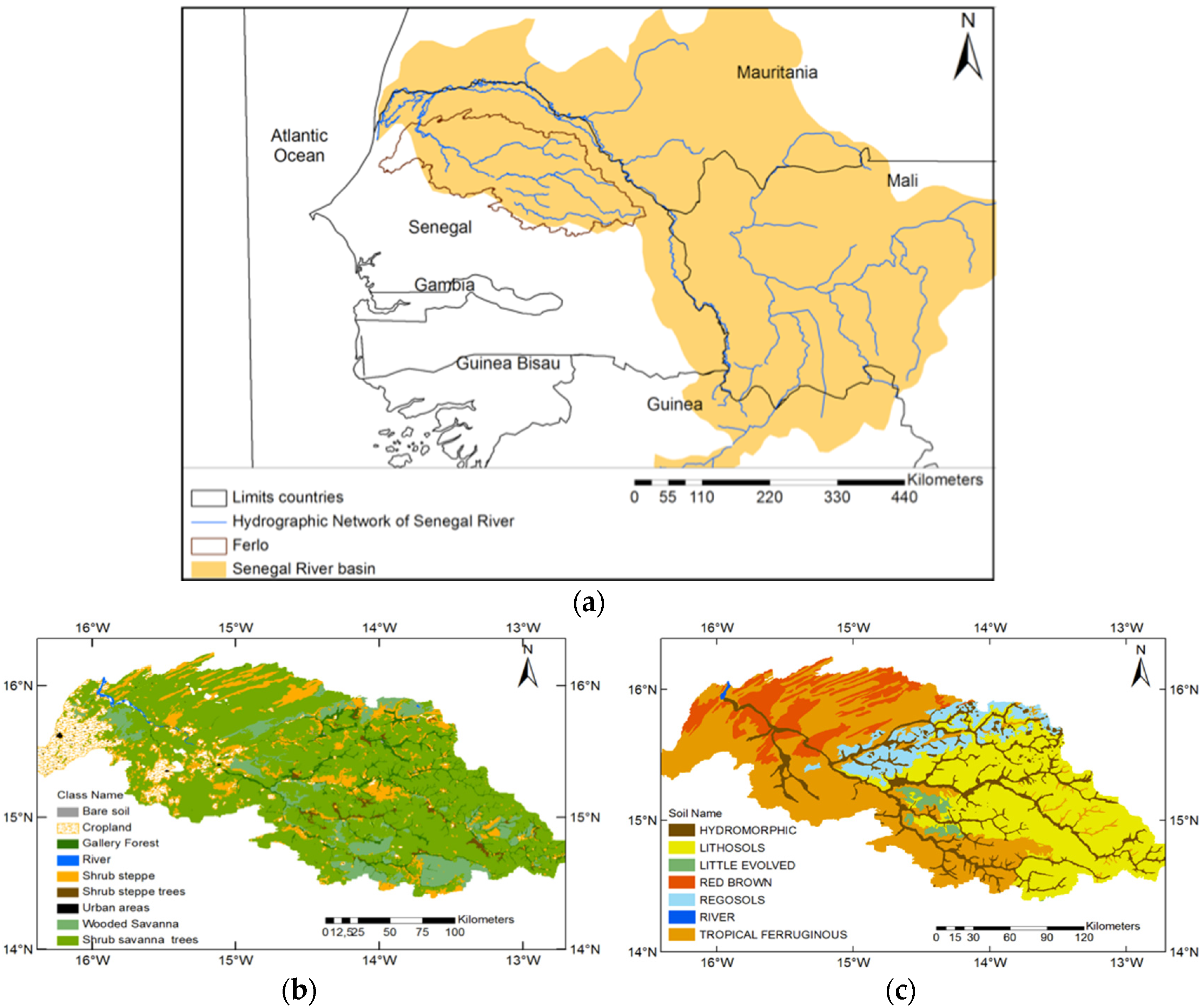
2.1. Study Area

The Ferlo basin is located in the north-central part of the Senegalese Sahelian climate zone between latitudes 14°30′N and 16°15′N and longitudes 12°50′W and 16°W (Figure 1a). The Ferlo River is a tributary of the Senegal River; during the rainy season it flows into the Senegal River via the Guiers Lake. According to Tappan et al. [14], three eco-regions are represented within the Ferlo basin:

• the northern sandy pastoral region (24,763 km²) where the predominant soils are red-brown sandy soils and ferruginous tropical sandy soils, covered by open shrub steppes and grasslands. On average, tree and shrub canopy cover does not exceed 5% of the total area, and the pseudo-steppe consists of a discontinuous herbaceous cover of annual grasses;
• the ferruginous pastoral region (30,908 km²) where soils are mainly shallow loamy and gravelly ferruginous tropical soils and lithosols on the plateau, and deep, sandy-to-loamy, leached tropical ferruginous soils in the valleys, the vegetation being characterized by shrub savanna, and bushland, often relatively dense. The herbaceous layer comprises a mix of annual and perennial grasses, leguminous species and other plants;
• the southern sandy pastoral region (10,852 km²) where the predominant soils are ferruginous tropical sandy soils, slightly leached, and covered by shrubs and tree savanna. In the wetter, southern part of the region, species diversity increases and the tree species become more abundant [14]. The herbaceous layer is dominated by leguminous species.

Table 1 and Table 2 summarize the soil characteristics and main vegetation species, following [14,15,16].

Figure 1. (a) Location of the Ferlo watershed study area; (b) land-cover map obtained from the FAO for 2005 [17] (Centre de Suivi Écologique (CSE), Dakar); (c) Soil type map extracted from the Senegalese Plan National d’Aménagement du Territoire (PNAT) published in 1986.

Figure 1. (a) Location of the Ferlo watershed study area; (b) land-cover map obtained from the FAO for 2005 [17] (Centre de Suivi Écologique (CSE), Dakar); (c) Soil type map extracted from the Senegalese Plan National d’Aménagement du Territoire (PNAT) published in 1986.

Table 1. Description of the five main soil types in the Ferlo watershed derived from the Plan National d’Aménagement du Territoire (PNAT) map of Senegal soils in 1986 (from Centre de Suivi Écologique (CSE), Dakar).

Soils	Description
Ferruginous Tropical soils	Found on the western and southern part with a sandy and clayey-sandy texture; they have a red color and are poor in organic matter. The soil surface is degraded as a result of exploitation and the absence of fallow periods. They usually have a low level of organic matter.
Hydromorphic soils	Found in the Ferlo valley and its former tributaries, they have variable textural features ranging from sandy silt to clayey silt. Their development is linked to a slight deficiency of drainage, which allows a certain accumulation of organic material.
Regosols soils	Very shallow and little evolved; they generally occupy the lower slopes in association with lithosols. They have low organic matter content.
Lithosols soils	Cover practically all of eastern Ferlo, they are raw mineral soils formed by non-climatic erosion of hard rock. They have low organic matter content.
Brown Red soils	Located in northern and western Ferlo on low plateaus and fixed dunes, they are characterized by poor organic matter content and low chemical fertility, they consist mainly of sand and clay. These soils have a red-brown color with low organic matter content uniform over much of the profile.

Table 1. Description of the five main soil types in the Ferlo watershed derived from the Plan National d’Aménagement du Territoire (PNAT) map of Senegal soils in 1986 (from Centre de Suivi Écologique (CSE), Dakar).

Soils	Description
Ferruginous Tropical soils	Found on the western and southern part with a sandy and clayey-sandy texture; they have a red color and are poor in organic matter. The soil surface is degraded as a result of exploitation and the absence of fallow periods. They usually have a low level of organic matter.
Hydromorphic soils	Found in the Ferlo valley and its former tributaries, they have variable textural features ranging from sandy silt to clayey silt. Their development is linked to a slight deficiency of drainage, which allows a certain accumulation of organic material.
Regosols soils	Very shallow and little evolved; they generally occupy the lower slopes in association with lithosols. They have low organic matter content.
Lithosols soils	Cover practically all of eastern Ferlo, they are raw mineral soils formed by non-climatic erosion of hard rock. They have low organic matter content.
Brown Red soils	Located in northern and western Ferlo on low plateaus and fixed dunes, they are characterized by poor organic matter content and low chemical fertility, they consist mainly of sand and clay. These soils have a red-brown color with low organic matter content uniform over much of the profile.

Table 2. Main vegetation species found in the Ferlo basin.

Vegetation Type	North to Center Ferlo	South Ferlo
Tree and bush species	Acacia seyal	Guiera senegalensis
	Combretum micrathum (kinkéliba)	Combretum glutinosum
	C. glutinosum
	C. nigricans
	Pterocarpus lucens
	Guiera senegalensis
	Feretia apodanthera
	Grewia bicolor
	Pterocarpus lucens
Herbaceous species	Dactyloctenium aegyptium,	Zornia glochidiata Reichb
	Aristida mutabilis	Alysicarpus ovalifolius
	Cenchrus biflorus	Indigofera senagalensis
	Schoenefeldia gracilis
	Tribulis terrestris
	Cassia obtifolius
	Zornia glochidiata.

Table 2. Main vegetation species found in the Ferlo basin.

Vegetation Type	North to Center Ferlo	South Ferlo
Tree and bush species	Acacia seyal	Guiera senegalensis
	Combretum micrathum (kinkéliba)	Combretum glutinosum
	C. glutinosum
	C. nigricans
	Pterocarpus lucens
	Guiera senegalensis
	Feretia apodanthera
	Grewia bicolor
	Pterocarpus lucens
Herbaceous species	Dactyloctenium aegyptium,	Zornia glochidiata Reichb
	Aristida mutabilis	Alysicarpus ovalifolius
	Cenchrus biflorus	Indigofera senagalensis
	Schoenefeldia gracilis
	Tribulis terrestris
	Cassia obtifolius
	Zornia glochidiata.

2.2. Satellite Data

The decade beginning in 2000 was selected for this study because the available satellite products are of the highest quality in terms of the number of observations (including time and space sampling) and accuracy. The LAI, rainfall and SM products used in this work are described in the following sections.

2.2.1. LAI

LAI is defined as the green leaf surface area of a canopy per unit of ground surface (m²∙m⁻²). It can be provided from MODIS (TERRA and AQUA) instruments [18,19,20,21,22] available at [23]. The MODIS LAI composite product [24] is available every eight days with a spatial resolution of 1 km². It is projected onto a 10° sinusoidal grid and is distributed in HDF-EOS format. The product is subjected to extensive quality control and has been found to work well in the Sahel [25], with a minimum uncertainty of about ± 0.2 m²∙m⁻² during the dry season ([14,24]). Zhang et al. [26] also used this product to monitor the vegetation growth. For Fensholt et al. [27], MODIS LAI data reproduce "the real world LAI" with R² ranging between 0.23 and 0.98 in a semi-arid savanna (in the center and north of Senegal). The product quality has been checked by comparing MODIS LAI and in situ measured LAI for semi-arid woodland and savanna in southern Africa [28]. The MODIS LAI data proved to be effective for phenology monitoring [29,30]. The MODIS dataset used in this work covers the period from February 2000 to December 2010.

2.2.2. Rainfall

The TRMM3B42 (Tropical Rainfall Measuring Mission) [31] product is available for the 50°N–50°S latitude band, at a spatial resolution of 0.25° × 0.25° and a time-step of three hours. The derived rainfall is based mainly on microwave measurements from the TRMM mission (Microwave Imager TMI, Precipitation Radar PR), complemented with measurements from other platforms (Special Sensor Microwave/Imager (SSMI) on the Defense Meteorological Satellite Program (DMSP) satellite series, the Advanced Microwave Scanning Radiometer-Earth Observing System (AMSR-E) on AQUA, and the Advanced Microwave Sounding Unit-B (AMSU-B) on the National Oceanic and Atmospheric Administration (NOAA) satellites). In addition, infrared data from geostationary satellites provide information on the precipitation cloud life, obtaining full coverage of the tropical latitudes. Data from the years 2000 to 2010 are used in this study.

The RFE 2.0 (African Rainfall Estimates Version 2.0) product [32] has a spatial resolution of 0.1° × 0.1° and a daily time-step. It covers from 40°S to 40°N and from 20°W to 55°E—the entire African continent. RFE 2.0 data are based on the combination of daily Global Telecommunication System (GTS) rain gauge data that consist of about 1000 rain gauges in Africa, as well as Advanced Microwave Sounding Unit (AMSU) and Special Sensor Microwave/Imager (SSM/I) satellite rainfall estimates. RFE 2.0 uses additional techniques to better estimate precipitation while continuing the use of cloud top temperature and station rainfall data, which formed the basis of RFE 1.0. Meteosat 7 geostationary satellite infrared data and are acquired at 30-min intervals, and areas depicting cloud top temperatures of less than 235 K are used to estimate convective rainfall. Both estimates are acquired at six-hour intervals and have a resolution of 0.25 degrees. Finally, daily rainfall is estimated by combining all satellite data using a maximum likelihood estimation method. GTS station data are then used to remove bias. Warm cloud precipitation estimates are not included in RFE 2.0. The database starts in October 2000, so all applications of this product in this study are for the period 2001–2010.

Both TRMM3B42 and the RFE 2.0 products can be used to evaluate the quality of the rainy season in the Sahel, as for example by Samimi et al. (2012) [33]. The major difference between them is that RFE 2.0 incorporates data from rain gauge measurements [34], whereas TRMM3B42 does not. These two daily products have been used in many previous studies across Africa analyzing precipitation [35], and TRMM3B42 data have been used to study the response of vegetation phenology to rainfall [36]. This product also showed good skill at estimating intense tropical cyclone rainfall [35] and at flood prediction [37]. RFE 2.0 data were also evaluated for Uganda in East Africa using a network of 27 rain gauges [38], showing that RFE 2.0 and two other satellite products (GPCP-1DD and TAMSAT) had similar characteristics and a high level of skill compared to model outputs (ERA-40 and ERA-Interim).

2.2.3. Soil Moisture

SM is defined as the water present in the unsaturated part of the soil profile, i.e., between the soil surface and the water table (e.g., [39,40]). Several studies have stressed the important role of SM in the water cycle (e.g., [41]) and in vegetation development (e.g., [42,43]).

The SM dataset used in this study is derived from microwave measurements, with both active and passive sensors, SMMR, SSM/I, TMI and ASMR-E (for the passive products) and the ERS and ASCAT scatterometers (for the active products) [44,45,46]. The signals from microwave sensors are related to SM in the upper few centimeters of the soil but the relationships between SM at the surface and in the root zone are well established (e.g., [45]). The SM product, in volumetric (m³∙m⁻³) units, has a spatial resolution of 0.25° × 0.25° and a daily time-step. It is available at [47]. Its validation has benefited from the increasing number of in situ datasets, many of them resulting from the initiative of the International Soil Moisture Network (available at [48]) [39], including 596 sites distributed through 28 SM networks worldwide [49].

2.3. Methodology

The challenge in this study is to interpret satellite data at a smaller scale compared to the horizontal resolution of the rainfall and SM data, and to incorporate local surface properties. With this aim, the Ferlo area was divided into homogeneous sub-areas, each with a unique set of parameters (soil-vegetation), in which the variabilities of the rainfall and vegetation growth can be analyzed individually.

2.3.1. Surface Classification

Land Cover

The land-cover classification (Figure 1b) was derived from a set of Landsat 5 images acquired by the TM sensor in November 2010 and geometrically corrected. This month corresponds to the end of the rainy season and to the end of vegetation growth. The data were obtained from [50] and were processed to produce a single mosaic image. A geographic information system (GIS) was then used to classify the Ferlo region into homogeneous zones by visual interpretation. The classification obtained was then compared with the Food Agricultural Organization (FAO) land-cover classification (available at: [17]) that also makes use of aerial photographs and socio-economic data. The two classifications were found to be consistent, although the FAO map includes a larger number of classes. Finally, a three-class classification corresponding to the dominant natural vegetation types, namely: shrub-steppe with trees (SStT), tree-savanna (TSv) and tree-savanna with shrubs (TSvS) was implemented.

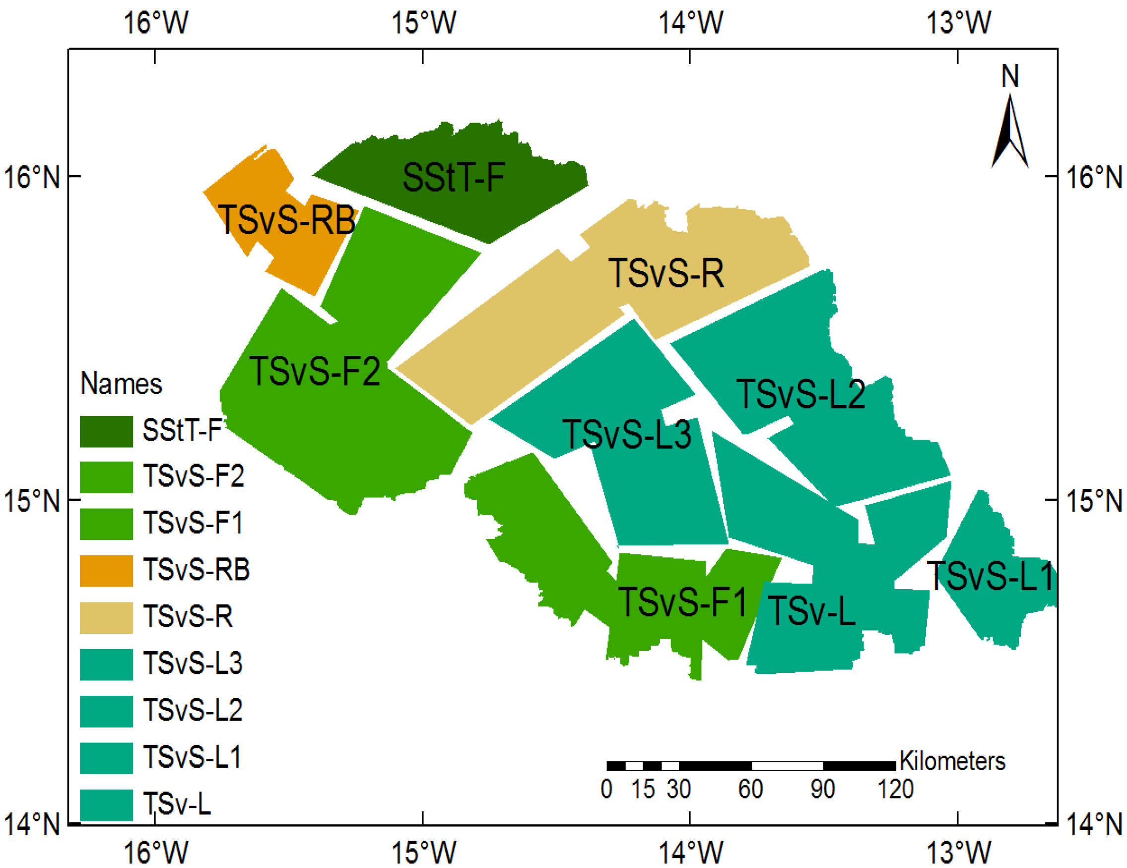
Homogeneous-Zone Characterization

A map (Figure 1c) of the main soil types was obtained from the Senegalese Plan National d’Aménagement du Territoire (PNAT) [51] (available from Centre de Suivi Ecologique, Dakar, Senegal). Using a GIS, soil type and vegetation classification maps were projected onto the same coordinate system. With these maps over-imposed, the polygons in which at least 100 LAI pixels (areas larger or equal to 100 km²) of a nearly single type of vegetation on a unique soil type were identified, following the above classification (Figure 2). These homogeneous vegetation-soil zones (VSZs) are described in Table 3. Their names are based on their vegetation and soil types. Because of these criteria, some non-homogeneous areas (river valleys and small cropland areas mostly found in transition zones) were filtered out, explaining the discontinuous patterns in Figure 2. In particular, the hydromorphic soils were not considered because continuous hydromorphic areas do not reach the threshold of 100 LAI pixels. Note that the soil-type homogeneity was taken as stronger criteria than the vegetation type, because the vegetation-type tree savanna with shrubs dominates most of the Ferlo.

Figure 2. Vegetation-Soil Zones (VSZ) map obtained from the superposition of the land-cover and soil-type maps, the heterogeneous transition zones were masked. The legend items are spelled out in Table 3.

Figure 2. Vegetation-Soil Zones (VSZ) map obtained from the superposition of the land-cover and soil-type maps, the heterogeneous transition zones were masked. The legend items are spelled out in Table 3.

Table 3. Abbreviations for the different vegetation-soil zones (VSZ) obtained from combining maps of vegetation types and maps of soil types.

Abbreviation	Description
TSvS-L1	Tree-Savanna with Shrubs (TSvS) on lithosols Soils (L)
TSv-L	Tree-Savannah (TSv) on lithosols Soils (L)
TSvS-L2	Tree-Savanna with Shrubs (TSvS) on Lithosols soils (L)
TSvS-F1	Tree-Savanna with Shrubs (TSvS) on Ferruginous tropical soils (F) in southeast sub-region
TSvS-L3	Tree-Savanna with Shrubs (TSvS) on Lithosols soils (L)
TSvS-R	Tree-Savanna with Shrubs (TSvS) on Regosol soils (R)
TSvS-F2	Tree-Savanna with Shrubs (TSvS) on Ferruginous tropical (F) in northwest sub-region
TSvS-RB	Tree-Savanna with Shrubs (TSvS) on Red-Brown soils (RB)
SStT-F	Shrub-Steppe with Trees (SStT) on Ferruginous tropical (F)

Table 3. Abbreviations for the different vegetation-soil zones (VSZ) obtained from combining maps of vegetation types and maps of soil types.

Abbreviation	Description
TSvS-L1	Tree-Savanna with Shrubs (TSvS) on lithosols Soils (L)
TSv-L	Tree-Savannah (TSv) on lithosols Soils (L)
TSvS-L2	Tree-Savanna with Shrubs (TSvS) on Lithosols soils (L)
TSvS-F1	Tree-Savanna with Shrubs (TSvS) on Ferruginous tropical soils (F) in southeast sub-region
TSvS-L3	Tree-Savanna with Shrubs (TSvS) on Lithosols soils (L)
TSvS-R	Tree-Savanna with Shrubs (TSvS) on Regosol soils (R)
TSvS-F2	Tree-Savanna with Shrubs (TSvS) on Ferruginous tropical (F) in northwest sub-region
TSvS-RB	Tree-Savanna with Shrubs (TSvS) on Red-Brown soils (RB)
SStT-F	Shrub-Steppe with Trees (SStT) on Ferruginous tropical (F)

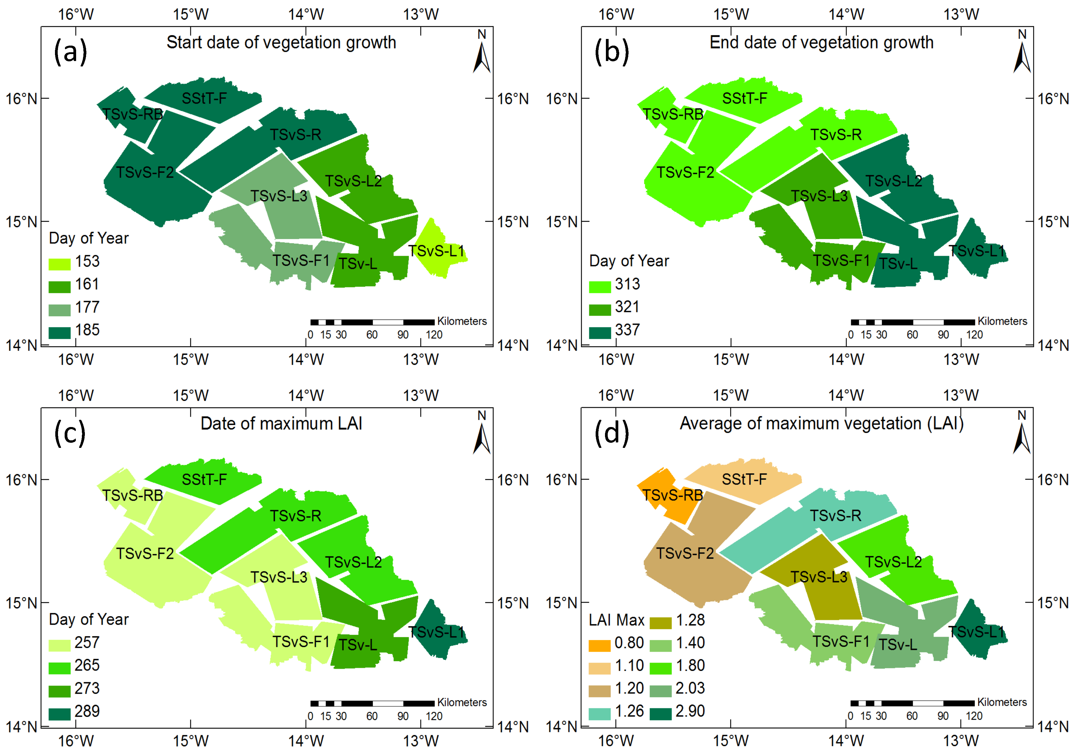
2.3.2. Vegetation Phenology Parameters

The phenological cycle in the Sahel is characterized by rapid vegetation growth at the end of June, following the monsoon onset, a maximum biomass (and LAI) in September, and a senescence phase through until the end of December. Even during the period of maximum variation of LAI within a VSZ (as expressed by the standard deviation), the 10% extreme values in the VSZ make a negligible impact on the mean LAI. Therefore, in the following, only the mean LAI values over the total area of each VSZ will be used. However, within-season temporal variations in LAI do result from the monsoon variability: in particular, marked decreases in LAI are observed every year during the growth phase. Phenological indicators such as the dates of the start and end for the growing season, and the maximum of the vegetation growth (date and amplitude) can be used to analyze the vegetation intra-seasonal and inter-annual variations.

Several methods have been proposed for determining these phenological dates, such as the sigmoid [25], the Gaussian Asymmetric (AG), and the Savitzky-Golay (SG) ([22,52]) functions. However, these methods do not allow one to globally adjust the phenological cycle. Chen et al. [53] proposed a Locally Adjusted Cubic-spline Capping (LACC) method to smooth the LAI image from the MODIS (MOD15A2) product. Following this approach, a cubic spline weighted by the inverse of the normalized variance was used within the VSZ. As a result, LAI time series were fitted and phenological dates were determined with the first and last curvature maxima corresponding to the start date of the growing season and to senescence, respectively. The maximum of LAI corresponds to the minimum curvature. Variations within the season are evaluated as anomalies with respect to the 11-year climatology, to which a three-point moving window is applied to remove the residual small-scale variability.

2.3.3. Soil Moisture

The dates defining the SM seasonal variations, i.e., start and end day of the wet period, are detected using a cubic-spline fit. As with LAI, the start and end days are estimated as the days with the first (and last) curvature maximum, and dry spells are defined as negative anomalies with respect to the 11-year climatology.

2.3.4. Rainfall Parameters

Three parameters were computed to characterize the rainy season and its intra-seasonal variation, namely: the onset and end dates of the rainy season, and the total rainfall amount during the vegetation growth season (June through September). At the intra-seasonal scale, the most important feature is the occurrence of dry spells.

Several methods have been developed to determine the dates of onset and end of the rainy season. Here, we applied the method of Odekunle [54] that defines the start date of the rainfall as the first positive point of maximum curvature of the cumulative precipitation. The end of the rainy season is defined as the latest date in the year when the daily rainfall is just greater than that which fell on the first rain day of the season. A rainfall threshold is required to detect dry spells during the rainy season, because statistical rainfall retrieval methods are inherently uncertain for low precipitation. This threshold may be defined differently according to the scientific discipline (meteorologist, agronomist or hydrologist) and the data source (local data or satellite data). Here, we define dry spells as occurring when the rainfall is less than or equal to 0.8 mm per day for TRMM3B42 and 0.5 mm per day for RFE 2.0 during a period of at least seven consecutive days.

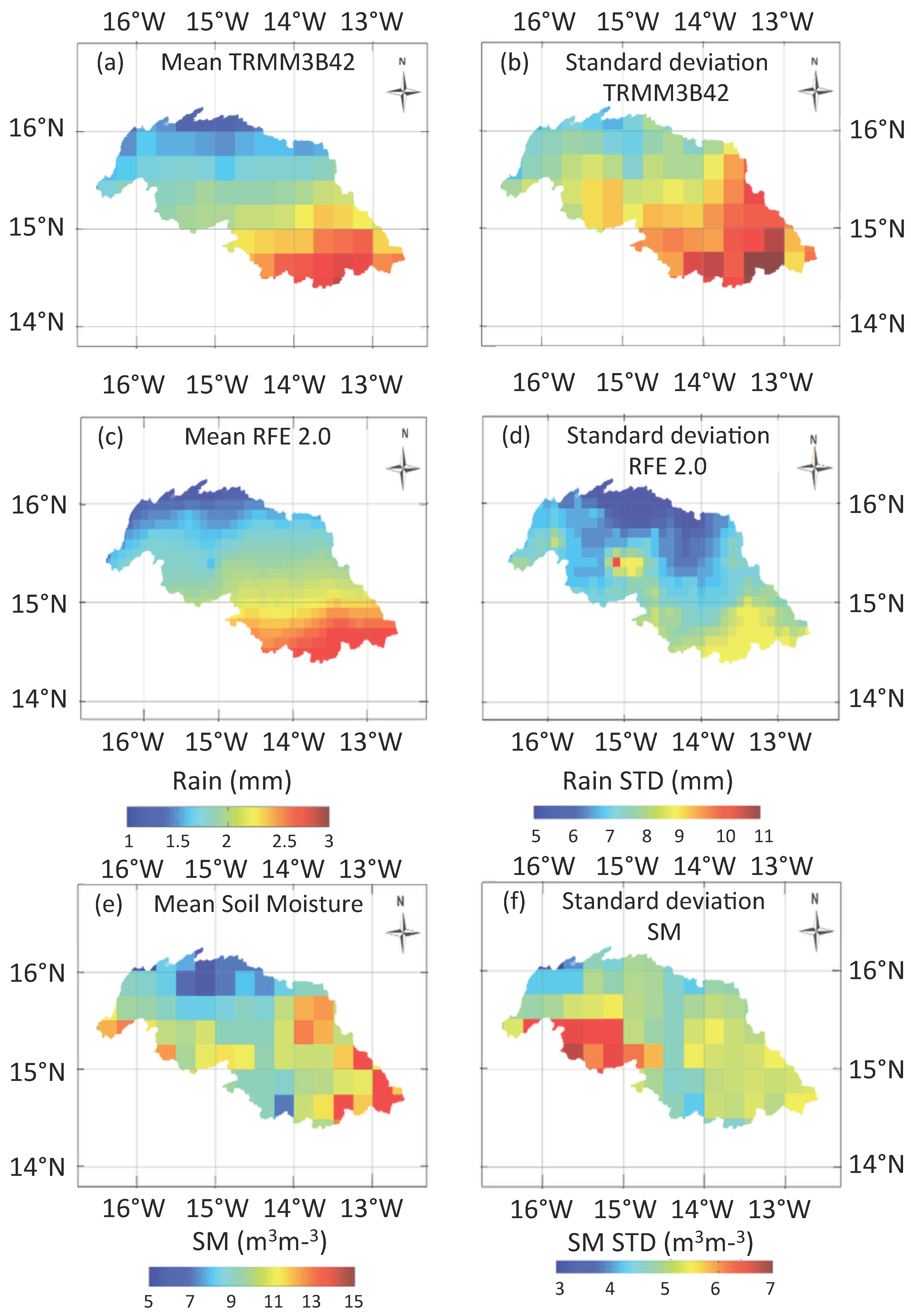
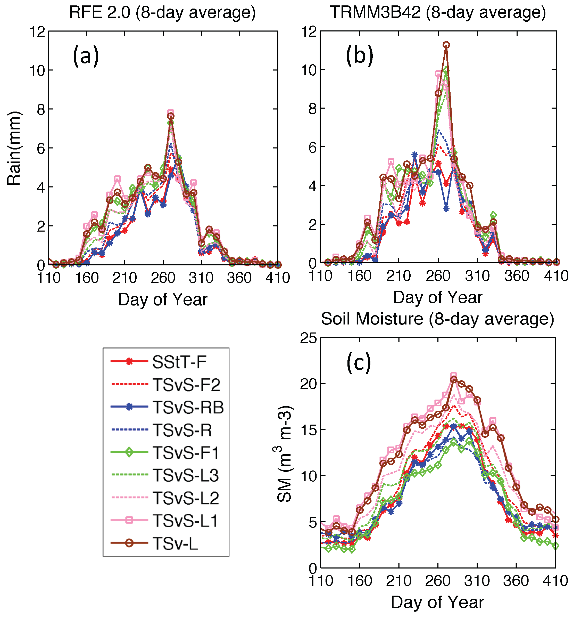
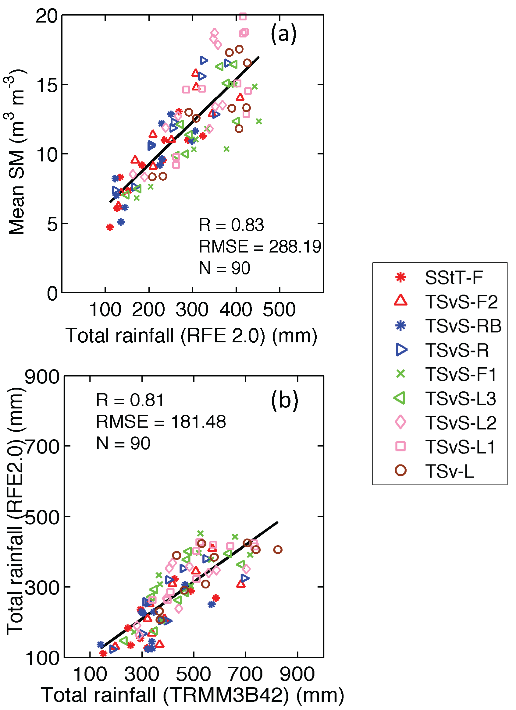
2.3.5. Comparison of TRMM3B42 and RFE 2.0 Products

Figure 3 presents the average rainfall and SM, and their standard deviations for the 2000–2010 decade. The two satellite products show similar spatial distributions of total rainy season rainfall. Although the mean maps present a picture of overall agreement (Figure 3a,c,e), the spatiotemporal variations (Figure 3b,d,f and Figure 4) show that the TRMM3B42 product displays much higher variation, particularly in the southeast. TRMM3B42 and RFE 2.0 standard deviations differ by a factor of approximately two. Despite an observed intensity difference, with higher maxima in the southern VSZs for TRMM3B42 (Figure 4), the two products are well correlated when comparing the yearly cumulated rainfalls of all VSZs over 10 years (Figure 5b). These results are consistent with previous work [34], which has shown that RFE 2.0 underestimates rainfall amount compared to the TRMM product. In their validation of satellite-based precipitation products, Thiemig et al. [55] show that RFE 2.0 and TRMM 3B42 present the best performance when compared to other products such as CMORPH [56], GPROF 6.0 [57].

Figure 3. Spatial variations of rainy season rainfall (i.e., for months June through September) from 2000 to 2010, (a–c) show 11-year average seasonal rainfall from TRMM3B42 and 10-year average for RFE 2.0, and 11-year average soil moisture; (d–f) quantify the year-to-year variability with the standard deviations.

Figure 3. Spatial variations of rainy season rainfall (i.e., for months June through September) from 2000 to 2010, (a–c) show 11-year average seasonal rainfall from TRMM3B42 and 10-year average for RFE 2.0, and 11-year average soil moisture; (d–f) quantify the year-to-year variability with the standard deviations.

Figure 4. Average rainfall over eight-day intervals from (a) RFE and (b) TRMM; and (c) soil moisture for each Vegetation-Soil Zone (VSZ) averaged over the 2000–2010 decade (see Table 3 for legend items).

Figure 4. Average rainfall over eight-day intervals from (a) RFE and (b) TRMM; and (c) soil moisture for each Vegetation-Soil Zone (VSZ) averaged over the 2000–2010 decade (see Table 3 for legend items).

2.3.6. Use of the Satellite-Derived Soil Moisture for Depicting the Intra-Seasonal Rainfall Variation

Figure 4c shows the mean seasonal evolution of SM over each VSZ for the 2000–2010 time period. Consistent with the rainfall distribution throughout the season, minimum SM is observed in those VSZs found in the north (SStT-F, TSvS-RB, TSvS-F2), while maximum SM is found in the southeast (TSv-L, TSvS-L1, TSvS-L2). However, the SM spatial variations do not show the same clear NW-SE gradient found for the rainfall. The main reason is that, despite the weak orography, the SM distribution in Ferlo is also constrained by the watershed hydrology, as shown by Tarnavsky et al. [9]. At the scale of the VSZs, SM temporal variations are quite similar to those of rainfall (Figure 5), but with smoother variations. The maximum values of SM and rainfall occur between the middle and end of August with SM decreasing more slowly than rainfall in the drying phase.

For both TRMM3B42 and RFE2.0, a good correlation between the mean SM and cumulated rainfall over the growth period, for each year and each VSZ, was found, as shown in Figure 5 (r = 0.76 and r = 0.83 for TRMM3B42 and RFE 2.0, respectively) and Figure 6a. The major difference between rainfall and SM is that while SM is a continuous time series, rain occurs as a series of discrete events. On average, over all VSZs, the rainy season onset dates agree to within one day (around Day 158). The dates of maximum rain are close for both rain products (difference, on average, of less than three days), but maximum SM occurs 10 days later, after loss through infiltration, runoff and evapotranspiration (Figure 6b). Finally, the number of dry spells longer than one week, estimated from the three datasets, agree to within one spell (between two and three dry spells for RFE 2.0 and SM, between three and four for TRMM3B42), and the duration of the longest dry spell per year is, on average, 11 days (12 days for TRMM3B42). Following the rainfall spatial variations, the dry spells are shorter in the south than in the north.

There is thus good agreement between the seasonal and intra-seasonal characteristics of rain and SM (Figure 6) and the CCI-SM product seems to properly depict the effects of the major rainfall variations within the season.

Figure 5. The total amount of rain from June through September averaged for the period 2000–2010 over the area of each vegetation-soil zone (VSZ, see Table 3 for legend items): (a) comparison between RFE rainfall and the soil moisture, and (b) comparison between TRMM and RFE.

Figure 5. The total amount of rain from June through September averaged for the period 2000–2010 over the area of each vegetation-soil zone (VSZ, see Table 3 for legend items): (a) comparison between RFE rainfall and the soil moisture, and (b) comparison between TRMM and RFE.

Figure 6. Comparison between some parameters characterizing the rainy season from TRMM3B42, RFE 2.0 and soil moisture (SM) in average on each vegetation soil zone (VSZ, see Table 3 for legend items) over the 2000–2010 decade: (a) cumulative rainfall and SM; (b) dates of onset and maximum (respectively in dark and clear colors); (c) number of dry spells and (d) the longest dry spells).

Figure 6. Comparison between some parameters characterizing the rainy season from TRMM3B42, RFE 2.0 and soil moisture (SM) in average on each vegetation soil zone (VSZ, see Table 3 for legend items) over the 2000–2010 decade: (a) cumulative rainfall and SM; (b) dates of onset and maximum (respectively in dark and clear colors); (c) number of dry spells and (d) the longest dry spells).

3. Mean Patterns of the Rainfall and Vegetation Phenology

The seasonal evolution of rainfall and SM (Figure 4) highlights the differences between those VSZs in the southeast and those in the northwest: the maximum, around day 240, is clearly seen for the TSvS-L (1 to 3) areas, but less obviously for SStT-F and TSvS-RB. The northern Ferlo (SStT-F) is the driest, with rather low time variability. This is consistent with the rain climatology of the Sahel, whereby the rainy season is composed of local rainfall events, and mesoscale convective systems, propagating from east to west, linked with African Easterly Waves. In the south of the Sahel, local convection leads to a rather regular frequency of precipitation, but further north, local convective storms are scarce and rainfall only results from the few mesoscale systems which reach that part of the region. The standard deviation maps of seasonal rainfall therefore show a higher interannual variability in the southeast part of the region (Figure 3b,d). The maximum SM standard deviation is observed in the western part of Ferlo, near 15.5°W (Figure 3f), which is the only significant area with arable agriculture (see Figure 1b). However, the local rain and SM variations in the SE of TSvS-F2 are stronger than those expected from the mean rainfall gradient. The proximity of the Ferlo riverbed, with a confluence of three rivers, is possibly the cause: as shown by Tarnavsky et al. [9], SM and runoff are locally maximal, and Soti et al. [10] showed the sensitivity of ponds in this area to rain perturbations.

As with rainfall and SM, the mean weekly LAIs were computed for every year, and averaged over the decade. The mean vegetation phenological cycles extracted for each VSZ are shown in Figure 7a. A cubic spline was applied to remove the individual small-scale variability. Figure 7b shows the standard deviation of LAI calculated for each VSZ over the month of September (month of the maximum LAI and maximum variability) and Figure 8 summarizes the spatial variations of some characteristic parameters (start dates, end dates, dates and values of the maximum LAI) in the vegetation cycle. The TSvS-L1 zone presents the maximal values (mean LAI about 2.9 m²∙m⁻²) with a strong variability (standard deviation about ± 0.19), as well as the earliest onset date (Figure 8a). The opposite occurs in the TSvS-RB zone which has the lowest maximal LAI (about 0.8) with a low variability (standard deviation lower than ±0.05) (Figure 8a,b).

Figure 7. (a) Variations of the mean LAI smoothed with the cubic spline, each color representing a homogeneous vegetation-soil zone (VSZ, see Table 3 for legend items); (b) into box plot, the standard deviation of LAI (a red segment inside the rectangle shows the median, the “whiskers (black horizontal dash)” above and below the box show the minimum and maximum standard deviation and the blue box around the median is the lower quartile (median value of the lower half of the data) and the upper quartile (median value of the upper half of the data)) for each zone over the 2000–2010 decade.

Figure 7. (a) Variations of the mean LAI smoothed with the cubic spline, each color representing a homogeneous vegetation-soil zone (VSZ, see Table 3 for legend items); (b) into box plot, the standard deviation of LAI (a red segment inside the rectangle shows the median, the “whiskers (black horizontal dash)” above and below the box show the minimum and maximum standard deviation and the blue box around the median is the lower quartile (median value of the lower half of the data) and the upper quartile (median value of the upper half of the data)) for each zone over the 2000–2010 decade.

Figure 8a shows that LAI follows the same southeast-northwest gradient as rainfall and SM, as observed previously by Justice et al. [58]: in the southeast, the growing season starts earlier and the maximum is higher, whereas in the northwest the growth starts later and reaches a lower maximum (Figure 8a). On average, the vegetation season starts in June (on average day 160 in the southeast, but one month later day 180 in the northwest), and finishes in November (around day 329 in the southeast and day 313 in the northwest), i.e., a difference in the length of the phenological cycle of between two and three weeks between the southeast and northwest. The maximum LAI is reached earlier in the northwest than in the southeast (Figure 8c). The phenological cycle is longer (Figure 8b), and LAI is higher in the south, which is consistent with the higher total rainfall amount during the season. The date of maximum vegetation is observed between the end of September in the northwest and the end of October in the southeast. Another feature of the southeast of Ferlo is that LAI is never lower than 0.5 (see Figure 7a), even at the end of the dry season, providing evidence of the presence of evergreen vegetation. This is not observed in the northwest part of the region, as already noted in Section 2.1.

Figure 8. Spatial variations of some characteristic parameters in the vegetation phenological cycle over the period 2000 to 2010: (a) start of the growing season; (b) end of the growing season; (c) date of maximum LAI; and (d) the maximum value of LAI.

Figure 8. Spatial variations of some characteristic parameters in the vegetation phenological cycle over the period 2000 to 2010: (a) start of the growing season; (b) end of the growing season; (c) date of maximum LAI; and (d) the maximum value of LAI.

4. Intra-Seasonal Analysis of Vegetation Response

The rainfall comprises a succession of wet and dry periods within the season; the pattern of these periods directly affects SM and vegetation growth. Between its onset and end, the West African Monsoon system is driven by these fluctuations that define the active and inactive phases of the monsoon.

In the previous section, the mean effect of variations within the rainy season over the decade was examined. Now, the intra-seasonal variations and anomalies of rainfall, SM, and LAI are analyzed. How breaks in the rainy season impact the vegetation has been widely studied ([2,25,59,60,61,62]). However, these general relationships may not apply when plant growth is strongly influenced by very local and specific features (e.g., soil type, species composition).

4.1. Effect of Rainfall Anomalies on LAI Variations through the Season

Rainfall, SM and LAI anomalies were calculated for each VSZ by removing the 11-year average annual cycle from the yearly data. These averages were smoothed to reduce the small-scale variability using a moving window of three weeks. Rainfall and SM anomalies were recalculated at LAI dates (eight-day time-step) by averaging the daily data, then time series of the June–September anomalies were built over the 2000–2010 decade. Finally, lagged correlations with the corresponding LAI time series were calculated.

As rainfall does not have a Gaussian distribution, we evaluated the statistical significance of correlations by applying a Monte Carlo test at 90%. To do this, yearly time series of rainfall (or SM) anomalies were randomly distributed within the 10 years before calculating the correlations with the actual LAI time series. A thousand random changes were performed to evaluate the mean significance level to which the correlation is compared. Finally, the mean lag between the time series was estimated by averaging the lags with a significant correlation coefficient (larger than a given threshold). In these correlations, anomalies (positive and negative) were separately correlated to distinguish the impacts of wet and dry anomalies on the vegetation.

Figure 9 summarizes the results for all VSZs. The value of the correlation coefficient is given in the left-hand panels, and the mean lag in the right-hand panels. Upper panels are for positive anomalies; bottom panels are for negative ones.

Figure 9. Comparison of correlation coefficients and lags in number of weeks between anomalies of rainfall and SM, and anomalies of LAI (TRMM3B42/LAI (blue) and RFE/LAI (green) and SM/LAI (red)) over the period 2000-2010 and on all the VSZs (see Table 3 for legend items) in the Ferlo watershed; with (a) correlation coefficients between positive anomalies; (b) correlation coefficients between negative anomalies; (c) lags between positive anomalies and (d) lags between negative anomalies.

Figure 9. Comparison of correlation coefficients and lags in number of weeks between anomalies of rainfall and SM, and anomalies of LAI (TRMM3B42/LAI (blue) and RFE/LAI (green) and SM/LAI (red)) over the period 2000-2010 and on all the VSZs (see Table 3 for legend items) in the Ferlo watershed; with (a) correlation coefficients between positive anomalies; (b) correlation coefficients between negative anomalies; (c) lags between positive anomalies and (d) lags between negative anomalies.

4.1.1. Positive Anomalies (Rainfall or SM above the Mean)

The positive rainfall and SM anomalies are correlated with LAI anomalies for all VSZs except the TSvS-L1, for which no significant correlation was found. This is also the case in TSv for both TRMM3B42 and RFE 2.0, as well as in TSvS-L2 for RFE 2.0. For all but the lithosols zones, the mean lag is about two weeks. This means that the vegetation growth is increasing two weeks after the positive rainfall anomaly occurs. The longer time lag obtained for SM on these VSZs is doubtful, as it corresponds to a lower correlation coefficient compared to the other VSZs. When looking at the correlation plots, a flat correlation coefficient is observed for all lags. These VSZs are characterized by a larger value of LAI (even significant during the dry season) and higher amounts of incoming/available water (rainfall and SM), as presented in the previous sections.

4.1.2. Negative Anomalies (Rainfall or SM below the Mean)

The negative rainfall or SM anomalies are better correlated to LAI negative anomalies than positive ones: the correlation coefficient is larger with a difference of +0.1, on average, for the two rain datasets and SM. We note that a significant correlation is missing only in TSvS-L1, and only for TRMM3B42. Compared to positive anomalies, negative anomalies have a stronger effect on the vegetation, as they induce water stress. The correlation coefficients between negative anomalies are almost the same when using the two rainfall products but they are higher in the case of SM. For both anomaly types, the correlations with SM are slightly larger than with rainfall on most of the VSZs. The vegetation response is faster for SM compared to rainfall with an average lag of between one to two weeks and two to three weeks, respectively, over all areas. The time lag varies among the homogeneous VSZs. In general, the correlation coefficients calculated for ferruginous soils are greater than 0.5, whereas for lithosols, they are less than 0.50.

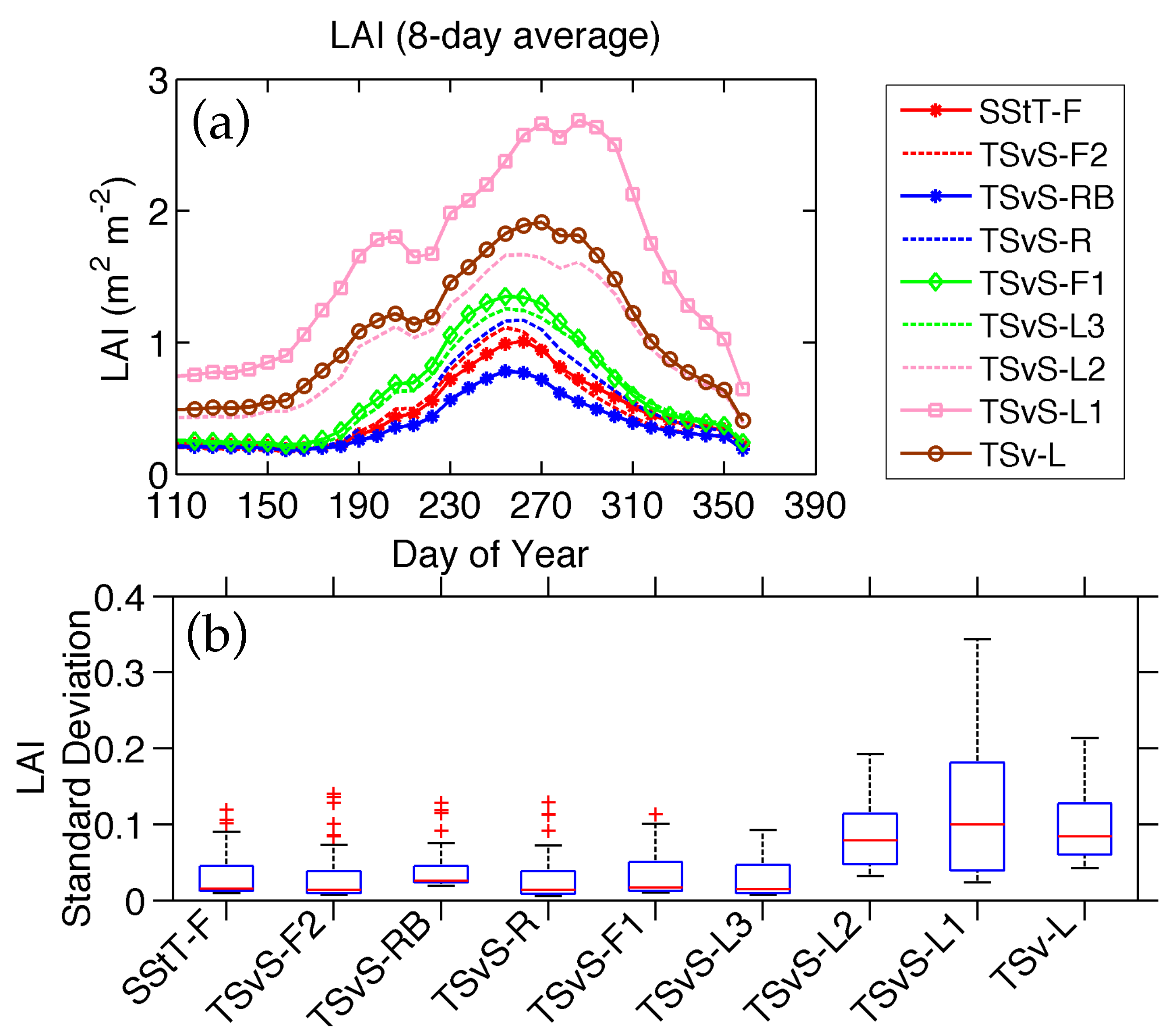
4.2. Impacts of Within-Season Rainfall and SM Variability on LAI

At the seasonal scale, the vegetation growth depends on the rainfall amount and its distribution during the rainy season. Water content in the root zone is the factor that most limits vegetation growth (e.g., [63,64]). The results of Section 4.1 indicate that rainfall anomalies impact vegetation growth. We now examine how the year-to-year variation could affect this correlation. To investigate the impact of rainfall anomalies within the season on the vegetation phenology, we examine the statistical relationships between LAI and selected rainfall-related indicators and investigate two questions:

-

Is the vegetation phenology (delay, amplitude) sensitive to the rainfall onset date?

-

Do the variations in the total rainfall amount have a similarly effect on all VSZs, and do the dry spells have a similar effect on the vegetation growth, whatever their date, number and duration?

To answer these questions, rainfall and SM were compared with LAI averaged over each VSZ, for every year. In these comparisons, rainfall, SM and LAI anomalies are all normalized relative to their maximum in each VSZ, in order to homogenize the overall VSZ variability.

The vegetation response relative to rainfall and SM indicators was analyzed using linear regression. The statistical significance of these relationships was evaluated using Student’s t-test, with a significance threshold of α = 5%. The anomalies within the season were calculated as the difference between each yearly time series and the smoothed average over the period 2000–2010, for each VSZ. Precipitation and SM time series were re-sampled with the same eight-day time-step as the LAI.

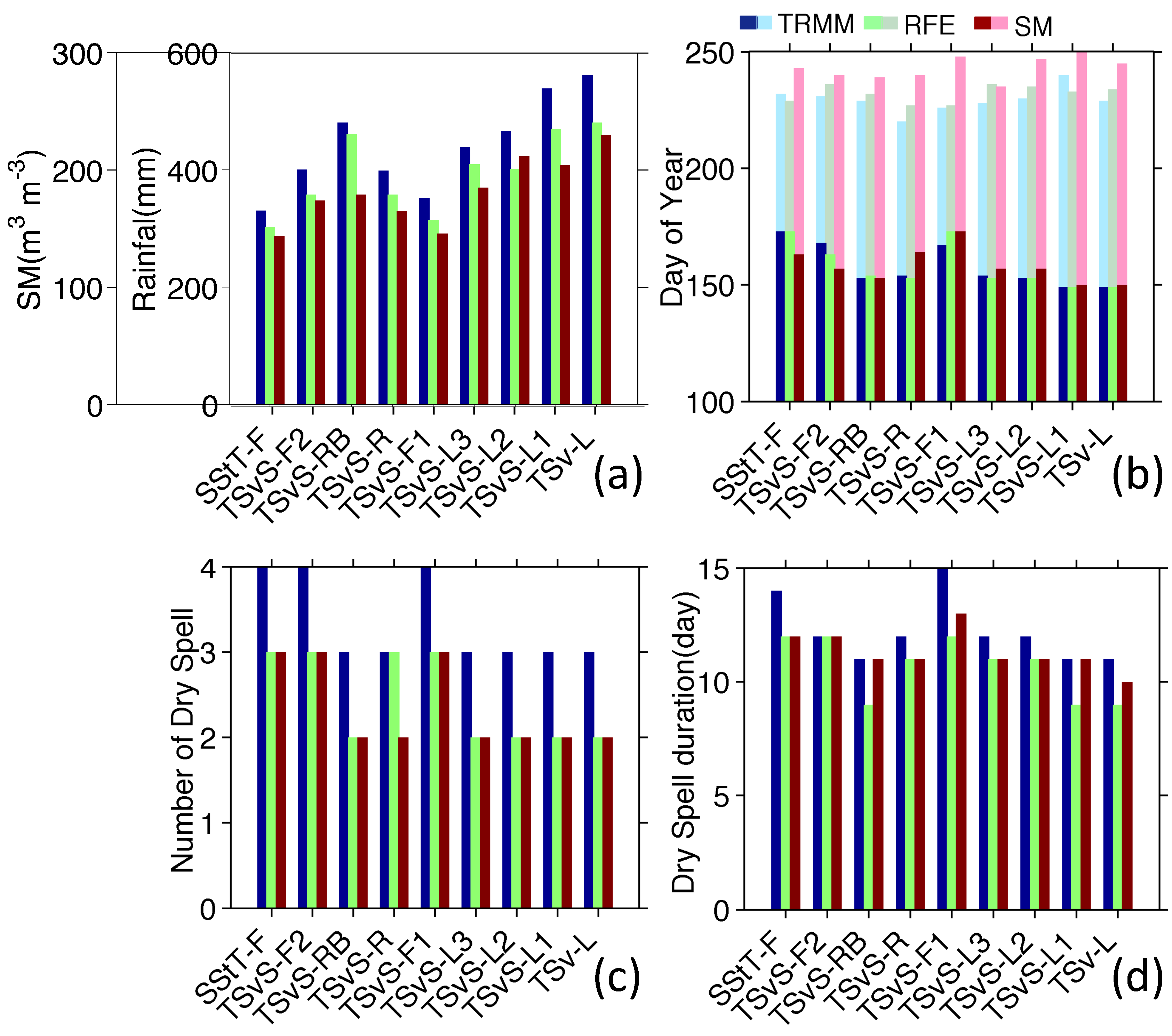
4.2.1. Rainy-Season Onset

To examine the impact of annual onset shifts with respect to the average date, we compared the difference between each season’s rainfall onset date and the mean rainfall onset date with the growing season start date and maximum LAI date (shifted with respect to the average date).

In zones with ferruginous soils, there is a fairly good correlation between the rainfall onset date and the start of the growing season (r = 0.54 and r = 0.51 for TRMM3B42 and RFE, respectively), significant by Student’s t-test. However, on the lithosols, these correlations are very low and not significant (r = 0.13 and r = 0.14).

However, the onset date of rainfall or SM does not affect the date of maximum LAI (no significant correlation). Thus, the phenological cycle is not delayed by late onset of the rainy season.

4.2.2. Rainfall Amount

The analysis of positive and negative rainfall anomalies has shown that the vegetation response is not the same for all the VSZs, with no significant coefficients on the lithosols. To investigate these differences, the links between total rainfall, mean SM and negative anomalies (number of dry spells; intensity of dry spells; duration of maximum dry spell; and intensity of maximum dry spell) and maximum of LAI were analyzed. For this, the lithosol and non-lithosol VSZs were separated. To give the same number of degrees of freedom in the statistical test, three ferrugineous and three lithosol VSZs were considered in both cases. Three thresholds on the duration of anomalies were used: ≥3 days; ≥5 days and ≥7days. Figure 10 summarizes the link between indicators of the rainfall amount variations and the vegetation growth up to the time of maximum LAI.

-

Total rainfall over the growing season (June–September):

The interannual correlations between the maximum LAI, total rainfall and SM for June–September (Figure 10a and Table 4) are significant (p < 0.05) on the non-lithosols soils with high correlation coefficients (r > 0.60 for TRMM; RFE 2.0 and SM), contrary to the lithosols, for which this relationship is not significant (p > 0.05 with r < 0.2).

-

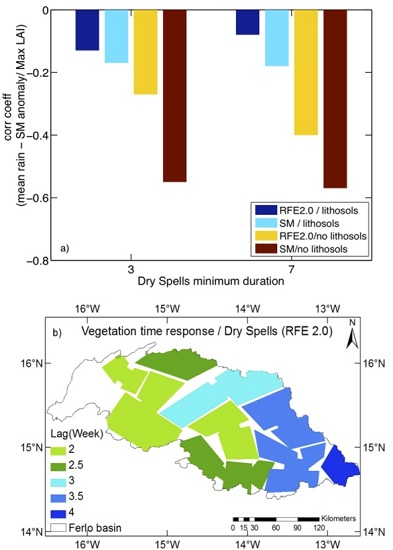
Impact of dry spells

To evaluate the impact of dry spell duration, number and intensity (rainfall anomaly with respect to the 11-year average) as well as SM negative anomalies on the yearly vegetation growth, three dry spell durations were explored: ≥3, ≥5 and ≥7 days (Figure 10).

A significant relationship was found for all zones other than those with lithosols. The correlations of the maximum LAI with SM anomalies (number and intensity) were all significant whatever the threshold on the duration of the dry spell, whereas the correlations with RFE 2.0 are significant only for the longest dry spell duration (≥7 days). Table 5 compares the longest SM anomaly duration and the maximum LAI for the three lithosols and the three ferruginous zones. For the latter, the correlation coefficients vary between −0.50 and −0.70, whereas they are not significant for the others. Similar results were found when correlating the anomaly intensity (cumulated over all dry spells, or only the longest one) with the maximum LAI. Again, the correlation is the largest with the SM anomaly amplitude compared with the anomalies derived from the two rainfall datasets. However, in addition to the soil type, the spatial distribution of dry spells is different (Figure 6), since the longest dry spells are localized in the northern part of Ferlo and have more impact in this sub-region than in the south.

Table 4. Inter-comparison of significant correlation coefficients between the total rainfall (TRMM3B42 and RFE 2.0), mean soil moisture (SM) and maximum LAI on each vegetation-soil zone (VSZ, see Table 3 for acronyms) over the period 2000 to 2010.

VSZ	Correlation Coefficient
	With TRMM	With RFE 2.0	With SM
TSvS-L1	--	--	--
TSv-L	--	--	--
TSvS-L2	--	--	--
TSvS-F1	0.61	0.47	0.53
TSvS-L3	0.56	0.30	0.32
TSvS-R	0.84	0.84	0.71
TSvS-F2	0.68	0.55	0.64
TSvS-RB	0.82	0.74	0.79
SStT-F	0.69	0.77	0.78

Table 4. Inter-comparison of significant correlation coefficients between the total rainfall (TRMM3B42 and RFE 2.0), mean soil moisture (SM) and maximum LAI on each vegetation-soil zone (VSZ, see Table 3 for acronyms) over the period 2000 to 2010.

VSZ	Correlation Coefficient
	With TRMM	With RFE 2.0	With SM
TSvS-L1	--	--	--
TSv-L	--	--	--
TSvS-L2	--	--	--
TSvS-F1	0.61	0.47	0.53
TSvS-L3	0.56	0.30	0.32
TSvS-R	0.84	0.84	0.71
TSvS-F2	0.68	0.55	0.64
TSvS-RB	0.82	0.74	0.79
SStT-F	0.69	0.77	0.78

Figure 10. Comparison of correlation coefficients between water availability and the maximum of vegetation growth on the Ferlo VSZs with (a) for non-lithosol VSZs and (b) lithosol VSZs over the period 2000–2010. TA: Total Amount; N-DS: Number of Dry Spells; I-DS: Intensity of Dry Spells; LDS-D: Longest Dry Spell Duration and LDS-I: Longest Dry Spell Intensity. The digits 3, 5 and 7 are the numbers of days corresponding to the thresholds of dry spell duration. The colors are dark blue for TRMM3B42; green for RFE 2.0 and dark red for SM. Horizontal solid and dashed lines correspond to the levels of significance for p < 5%.

Figure 10. Comparison of correlation coefficients between water availability and the maximum of vegetation growth on the Ferlo VSZs with (a) for non-lithosol VSZs and (b) lithosol VSZs over the period 2000–2010. TA: Total Amount; N-DS: Number of Dry Spells; I-DS: Intensity of Dry Spells; LDS-D: Longest Dry Spell Duration and LDS-I: Longest Dry Spell Intensity. The digits 3, 5 and 7 are the numbers of days corresponding to the thresholds of dry spell duration. The colors are dark blue for TRMM3B42; green for RFE 2.0 and dark red for SM. Horizontal solid and dashed lines correspond to the levels of significance for p < 5%.

Table 5. Significant correlation coefficients after application of the Student t-test with a 5% threshold between duration of dry spell (with SM) and maximum of LAI from (JJAS) and the corresponding Root Mean Square Error (RMSE) on each VSZ (see Table 3 for the acronyms).

VSZ	Significant Correlation Coefficients	RMSE
SStT-F	−0.71	3.29
TSvS-F2	−0.79	3.23
TSvS-F1	−0.54	4.34
TSvS-L3	—	4.31
TSvS-L2	—	4.63
TSvS-L1	—	4.52

Table 5. Significant correlation coefficients after application of the Student t-test with a 5% threshold between duration of dry spell (with SM) and maximum of LAI from (JJAS) and the corresponding Root Mean Square Error (RMSE) on each VSZ (see Table 3 for the acronyms).

VSZ	Significant Correlation Coefficients	RMSE
SStT-F	−0.71	3.29
TSvS-F2	−0.79	3.23
TSvS-F1	−0.54	4.34
TSvS-L3	—	4.31
TSvS-L2	—	4.63
TSvS-L1	—	4.52

5. Discussion

5.1. Significant Information from Rainfall and SM Products

The analysis shows that rainfall and SM have similar spatial variations, but with less temporal variability for SM. This can be expected since SM is an integrated variable, resulting from the surface partitioning of rainfall into evapotranspiration, surface runoff and infiltration. It has a slow temporal evolution.

Although TRMM3B42 and RFE 2.0 are direct estimates of the daily rainfall, the uncertainty in their variations, as seen when comparing the two databases, results in a similar uncertainty in the rainy season patterns at the scale of each VSZ. Despite the unknown source of these errors, SM properly depicts the overall rainfall seasonal variations and anomalies. An advantage of SM is that its relationship with the microwave radiometer measurement (variations of the surface emission linked to soil dielectric properties) is more direct than that for precipitation (conversion of instantaneous emission from droplets and crystals in the atmosphere into a cumulated surface amount). In addition, the SM variations are smoother than those of rainfall, because SM integrates the effect of sporadic rainfall events, with continuous surface processes. This makes it easier to determine season-to-season and within-season variations.

The correlation between cumulated rainfall over the growth season and the maximum LAI in that season is very similar for the three products: on the non-lithosols, it is larger than 0.6.

The major differences between products occur with the anomalies. The direct correlations of anomalies longer than seven days over the whole time range as well as correlations of yearly integrated indicators show differences between the three products:

-

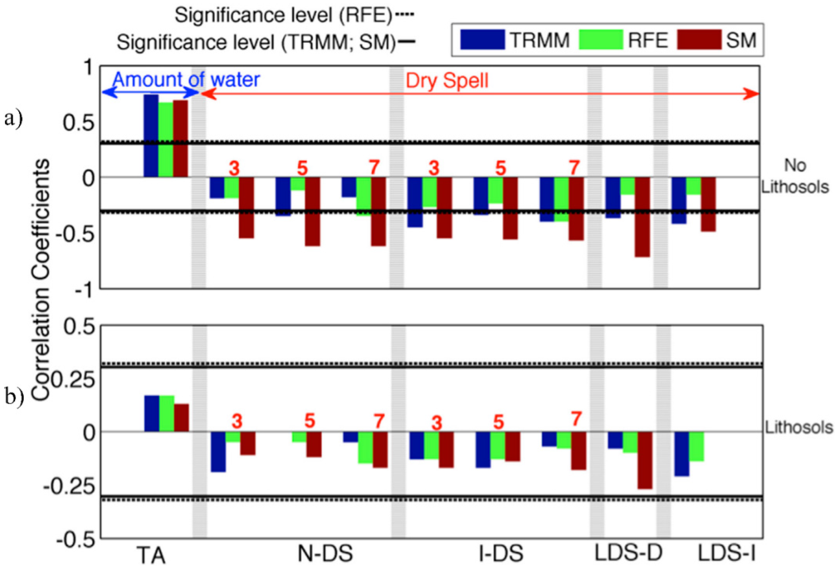
Correlations of both positive and negative anomalies are higher for SM and RFE 2.0 than TRMM3B42, except on lithosols. In addition, the time lag obtained with SM for negative anomalies is slightly smaller than for the two rainfall products.

-

Correlations of the cumulated water deficit, as well as the number of dry spells and the duration of the longest one, with maximum LAI were calculated to evaluate the impact of dry spells on the maximum LAI. Again, a significant correlation was found, except for lithosols. However, this correlation becomes significant for SM as soon as the dry anomaly is longer than three days, but is significant for both rainfall products only for anomalies longer than seven days. In general, a better correlation is obtained with TRMM3B42 than RFE 2.0 (for example, see the correlation for the longest dry spell).

In any case, SM appears to be a better indicator for detecting anomalies which impact the LAI. As noted earlier, an important source of uncertainty for rainfall comes from the discontinuous sampling of rainfall events, which are then summed to give a daily value. Thus, it is difficult to assess the significance of a three-day dry spell, which, in addition, depends on the threshold used on the rainfall products (see Section 2.3.3). On the contrary, any SM anomaly means that less water is available for the vegetation at the surface. Thus, SM anomalies are more directly linked to vegetation growth.

The direct correlation of rainfall anomalies with SM anomalies over the 2000–2010 time series shows a slight delay (by about one week). Thus, there is a more rapid response of vegetation to SM anomalies than to rainfall anomalies (on average two days of shift relative to the positive and negative anomalies of SM, between 2.5 to 3.5 days for negative anomalies, and between two to three days for positive anomalies of rain).

These results confirm earlier findings by Nicholson et al. [60] that vegetation greenness in semi-arid environments is more strongly related to SM, a function of rainfall accumulated over a period of time, than to instantaneous rainfall. Even if satellite-derived SM is a surface variable, its variations are more consistently related to vegetation growth compared to rainfall, because part of the rainfall will be lost as surface runoff, interception and soil evaporation, making the rainfall unrepresentative of the water transpired by the vegetation during photosynthesis.

5.2. Impact of the Intra-Seasonal Variations in the Rainy Season on the Vegetation Phenology

5.2.1. Impacts of Water Variability Across the Ferlo Basin

The maximum LAI map confirms the climatic gradient observed in rainfall and SM: the southeast has a denser savanna with a significant proportion of ligneous species (shrubs and trees); in contrast, the northwest vegetation is mainly composed of herbaceous species (see Table 1). This difference is linked to the overall water availability in the two sub-regions.

Consequently, the less dense and less watered northwest sub-region is more sensitive to intra-seasonal and seasonal variations. The rainfall and SM seasonal fluctuations strongly affect the northwest, as shown by the correlation coefficients all being greater than 0.50 for northern VSZs, unlike the southern ones (see, for example, the difference between non-lithosols and lithosols in Figure 10). The yearly indicators such as the maximum duration of dry spells strongly affect the vegetation growth in the northwest (r = −0.57), contrary to the southeast (r = −0.11). This difference can be attributed to the impact of local storms being more frequent in the southeast: SM is therefore greater and the vegetation is less sensitive to dry spells, being better able to cope with rainfall fluctuations (negative or positive).

The correlation between times series confirms the differences between northwest and southeast: correlation coefficients for both positive and negative anomalies are higher for VSZs in the northwest (see, for example, the differences between TSvSF2/TSvS-F1, TSvS-L3/TSvS-L1). In the extreme southeast, no correlation is obtained.

5.2.2. Role of Vegetation Cover and Soil Type

In the same climatic sub-zone, the LAI intensity on lithosols is higher than on ferruginous soils, even during dry spells. Moreover, the TSvS-L zones present two peaks of LAI unlike the others such as SStT-F. However, the observed differences cannot be attributed to the climatic gradient alone, as the vegetation also changes along this gradient, and the soil types are not homogeneously distributed within the Ferlo basin. As already presented, the vegetation is composed of trees, shrubs and herbaceous species. Sahelian vegetation is distinguished from that of other arid zones by the scarcity of perennial grasses [65] and in the northern part of the basin, shallow-rooted annual grasses dominate. In the southeast, ligneous species have a greater presence; these plants have roots that give them access to deep soil water or shallow groundwater.

The features of the woody savanna identified here may come from the presence of species such as microphyll for Acacia and sclerophyll for Boscia senegalensis. These species have an inverse phenological cycle of growth during the beginning of the rainy season, keeping their leaves throughout the dry season. They have well-developed mechanisms to reduce water loss through transpiration [65] and therefore perform better than herbaceous vegetation under water deficit conditions. These differences in plant physiology and architecture may explain the double peak in LAI seasonal variation. Thus, it is probable that annual grasses are the most sensitive to water input anomalies, with perennial grasses being more resilient, due to their deeper root system. Finally, the transpiration control and deep roots of shrubs and trees make them the most resilient to dry spell−induced water shortage.

The geographical position of the different soil types mixes the impact of soil properties with the climatic gradient effect. The correlation study confirms the differences between lithosols and ferruginous soils. The correlations between the rainfall onset date and the start of the vegetation-growing season on the ferruginous soils are significant (r > 0.50) by Student’s t-test (p < 0.05), whereas on lithosols soils they are lower and not significant (r = 0.13). On the ferruginous soils, vegetation responds more rapidly and more strongly. The correlations between rainfall and vegetation anomalies (positive and negative) confirm this difference between the soil types with correlation coefficients always being significant with ferruginous soils, but not with lithosols. To further elucidate the role of the soil type, we compared VSZs located in the same climatic area, mainly TSvS-F1 and TSvS-L3. Their phenological cycles and the response to within-season anomalies were very similar, but the correlations between the total rainfall and the maximum LAI were significantly lower for TSvS-L3 than TSvS-F1 (Table 4). Contrary to TSvS-F1, there was no significant correlation between the duration of the longest dry spell and the LAI maximum for TSvS-L3 (Table 5). Lithosols thus have a different response to the rainfall variations.

The above results could be explained by differences in infiltration rate between the two soil types. Infiltration through lithosols is slow because these soils are composed of hard rock that allows water to remain at the surface for a longer time, making it available for herbaceous vegetation. In contrast, for the other soils (ferruginous, red-brown, regosols), the faster infiltration makes the vegetation more sensitive to soil water availability. This might explain the weak or null response of lithosol VSZs to intra-seasonal rainfall anomalies. In addition, lithosols are located in the southeast where the flat topography leads to negligible surface runoff. Flat topography is more favorable to vegetation growth, resulting in denser savanna which recovers more strongly. These effects might explain the weak or null response of lithosol VSZs to intra-seasonal rainfall anomalies.

6. Conclusions

In this study, satellite data were used to evaluate the impact of intra-seasonal rainfall variations on the natural vegetation growth of a small region in the Sahel (Ferlo, Senegal). The Ferlo region was subdivided into nine zones, mainly homogeneous in terms of vegetation and soil type. These zones were sufficiently large to allow the use of rainfall, SM and LAI satellite products, but small enough to properly depict the spatial heterogeneity of the soil and vegetation cover.

First, two well-known rainfall products, RFE 2.0 and TRMM3B42, were compared over a 10-year period at the scale of the homogeneous zones. Despite differences in the cumulated rainfall amounts, TRMM3B42 and RFE2.0 were well correlated over the whole region. Both were also well correlated with the ESA CCI.SM product, although the mean variations over the rainy season are smoother than the rainfall ones. The three databases provide intra-seasonal variations, which were found to correlate with the variations in vegetation phenology. However, correlations with RFE 2.0 were found to be higher than with TRMM3B42; SM variations were found to be significantly more correlated to LAI (anomalies and maximum value) than rainfall variations. SM thus appears as the most relevant parameter for evaluating the impact of rainfall anomalies on vegetation growth. The within-season rainfall and SM anomalies are followed three weeks later (on average) by correlated anomalies in LAI. Dry spells are correlated with the maximum LAI. However, a significant response of the LAI is observed only when the absence of rainfall lasts more than seven days, whereas a three-day deficit of SM leads to a significant correlation. These results were validated over all soils except lithosols. In the latter case, most of the correlations failed to be significant.

Our study shows how the combined analysis of satellite-observed rainfall, SM and LAI can help to better understand the vegetation/rainfall relationship and to assess spatiotemporal variability in vegetation growth, in relation to soil type. The significant correlations obtained indicate that LAI is a “good index” of the quality of the monsoon season and that SM data can be used to monitor this indicator. The next step should thus be the building of a statistical prediction tool, which could be used to predict the vegetation biomass before the end of the growing season. To extend this study, the methodology should be incorporated into process-based vegetation growth models for evaluating the impacts of rainy season onset, cumulated rainfall and dry spells on the production of animal grazing and crops.

References

1. Lebel, T.; Ali, A. Recent trends in the Central and Western Sahel rainfall regime (1990–2007). J. Hydrol. 2009, 375, 52–64. [Google Scholar] [CrossRef]
2. Herrmann, M.S.; Anyamba, A.; Tucker, J.C. Recent trends in vegetation dynamics in the African Sahel and their relationship to climate. Glob. Environ. Chang. 2005, 15, 394–404. [Google Scholar] [CrossRef]
3. Nicholson, S.E.; Farrar, T.J. The influence of soil type on the relationships between NDVI, rainfall, and soil moisture in semiarid Botswana. I. NDVI response to rainfall. Remote Sens. Environ. 1994, 50, 107–120. [Google Scholar] [CrossRef]
4. Marteau, R.; Moron, V.; Philippon, N. Spatial coherence of monsoon onset over Western and Central Sahel (1950–2000). J. Clim. 2009, 22, 1313–1324. [Google Scholar] [CrossRef]
5. Ibrahim, B.; Polcher, J.; Karambiri, H.; Rockel, B. Characterization of the rainy season in Burkina Faso and it’s representation by regional climate models. Clim. Dyn. 2012, 39, 1287–1302. [Google Scholar] [CrossRef] [Green Version]
6. Barron, J.; Rockström, J.; Gichuki, F.; Hatibu, N. Dry spell analysis and maize yields for two semi-arid locations in east Africa. Agric. For. Meteorol. 2003, 117, 23–37. [Google Scholar] [CrossRef]
7. Frappart, F.; Hiernaux, P.; Guichard, F.; Mougin, E.; Kergoat, L.; Arjounin, M.; Lavenu, F.; Koité, M.; Paturel, J.E.; Lebel, T. Rainfall regime across the Sahel band in the Gourma region, Mali. J. Hydrol. 2009, 375, 128–142. [Google Scholar] [CrossRef] [Green Version]
8. Karlson, M.; Ostwald, M. Remote sensing of vegetation in the Sudano-Sahelian zone: A literature review from 1975 to 2014. J. Arid Environ. 2015, 124, 257–269. [Google Scholar] [CrossRef]
9. Tarnavsky, E.; Mulligan, M.; Ouessar, M.; Faye, A.; Black, E. Dynamic hydrological modeling in drylands with TRMM based rainfall. Remote Sens. 2013, 5, 6691–6716. [Google Scholar] [CrossRef] [Green Version]
10. Soti, V.; Puech, C.; lo Seen, D.; Bertran, A.; Vignolles, C.; Mondet, B.; Dessay, N.; Tran, A. The potential for remote sensing and hydrologic modelling to assess the spatio-temporal dynamics of ponds in the Ferlo Region (Senegal). Hydrol. Earth Syst. Sci. 2010, 14, 1449–1464. [Google Scholar] [CrossRef] [Green Version]
11. Beven, K.J.; Fisher, J. Remote sensing and Scaling in Hydrology, Scaling in Hydrology Using Remote Sensing. In Scaling Issues in Hydrology; Stewart, J.B., Engman, E.T., Fedds, A., Kerr, Y., Eds.; Wiley: Chichester, UK, 1996. [Google Scholar]
12. Gash, J.H.C.; Kabat, P.; Monteny, B.; Amadou, M.; Bessemoulin, P.; Billing, H.; Blyth, E.; DeBruin, H.; Elbers, J.; Friborg, T. The variability of evaporation during the HAPEX-Sahel Intensive Observation Period. J. Hydrol. 1997, 188, 385–399. [Google Scholar] [CrossRef]
13. Zribi, M.; Pardé, M.; de Rosnay, P.; Baup, F.; Boulain, N.; Descroix, L.; Pellarin, T.; Mougin, E.; Ottlé, C.; Decharme, B. ERS scatterometer surface soil moisture analysis of two sites in the south and north of the Sahel region of West Africa. J. Hydrol. 2009, 375, 253–261. [Google Scholar] [CrossRef] [Green Version]
14. Tappan, G.G.; Sall, M.; Wood, E.C.; Cushing, M. Ecoregions and land cover trends in Senegal. J. Arid Environ. 2004, 59, 427–462. [Google Scholar] [CrossRef]
15. Martinez, B.; Gilabert, M.A.; Garcia-Haro, F.J.; Faye, A.; Meliά, J. Characterizing land condition variability in Ferlo, Senegal (2001–2009) using multi-temporal 1-km Apparent Green Cover (AGC) SPOT VEGETATION data. Glob. Planet. Chang. 2011, 76, 152–165. [Google Scholar] [CrossRef]
16. Akpo, L.E.; Gaston, A.; Grouzis, M. Structure spécifique d’une végétation sahélienne. Cas de Wiidu Thiengoli (Ferlo, Sénégal). Bull. Mus. Natl. Hist. Nat. Paris 1995, 17, 39–52. [Google Scholar]
17. Land-Cover Map from FAO 2005. Available online: http://www.glcn.org/databases/se_landcover_en.jsp (accessed on 2 September 2015).
18. Myneni, R.B.; Hoffman, S.; Knyazikhin, Y.; Privette, J.L.; Glassy, J.; Tian, Y.; Wang, Y.; Song, X.; Zhang, Y.; Smith, G.R.; et al. Global products of vegetation leaf area and fraction absorbed PAR from year one of MODIS data. Remote Sens. Environ. 2002, 83, 214–231. [Google Scholar] [CrossRef]
19. Yang, W.; Shabanov, N.V.; Huang, D.; Dickinson, R.E.; Nemani, R.R.; Knyazikhin, Y.; Myneni, R.B. Analysis of leaf area index products from combination of MODIS TERRA and AQUA data. Remote Sens. Environ. 2006, 104, 297–312. [Google Scholar] [CrossRef]
20. De Kauwe, M.G.; Disney, M.I.; Quaife, T.; Lewis, P.; Williams, M. An assessment of the MODIS collection 5 Leaf Area Index product for a region of mixed coniferous forest. Remote Sens. Environ. 2011, 115, 767–780. [Google Scholar] [CrossRef]
21. Ruhoff, A.L.; Paz, A.R.; Aragao, L.E.O.C.; Mu, Q.; Malhi, Y.; Collischonn, W.; Rocha, H.R.; Running, S.W. Assessment of the MODIS global evapotranspiration algorithm using eddy covariance measurements and hydrological modelling in the Rio Grande basin. Hydrol. Sci. J. 2013, 58, 1–19. [Google Scholar] [CrossRef]
22. Yuan, H.; Dai, Y.; Xiao, Z.; Ji, D.; Shangguan, W. Reprocessing the MODIS Leaf Area Index products for land surface and climate modeling. Remote Sens. Environ. 2011, 115, 1171–1187. [Google Scholar] [CrossRef]
23. LAI MODIS Product. Available online: https://lpdaac.usgs.gov/dataset_discovery/modis/modis_products_table/mod15a2 (accessed on 12 May 2015).
24. Knyazikhin, Y.; Martonchik, V.; Diner, D.J.; Myneni, R.B.; Verstraete, M. Estimation of vegetation canopy leaf area index and fraction of absorbed photosynthetically active radiation from atmosphere-corrected MISR data. J. Geophys. Res. 1998, 103, 32239–32256. [Google Scholar] [CrossRef]
25. Bobée, C.; Ottlé, C.; Maignan, F.; de Noblet-Ducoudré, N.; Maugis, P.; Lézine, A.M.; Ndiaye, M. Analysis of vegetation seasonality in Sahelian environments using MODIS LAI, in association with land cover and rainfall. J. Arid Environ. 2012, 84, 38–50. [Google Scholar] [CrossRef]
26. Zhang, X.; Friedl, M.A.; Schaaf, C.B.; Strahler, A.H.; Liu, Z. Monitoring the response of vegetation phenology to precipitation in Africa by coupling MODIS and TRMM3B42 instruments. J. Geophys. Res. 2005, 110. [Google Scholar] [CrossRef]
27. Fensholt, R.; Sandholt, I.; Rasmussen, M.S. Evaluation of MODIS LAI, fAPAR and the relation between fAPAR and NDVI in a semi-arid environment using in situ measurements. Remote Sens. Environ. 2004, 91, 490–507. [Google Scholar] [CrossRef]
28. Privette, J.L.; Myneni, R.B.; Knyazikhin, Y.; Mukelabai, M.; Roberts, G.; Pniel, M.; Wang, Y.; Leblanc, S. Early spatial and temporal validation of MODIS LAI product in Africa. Remote Sens. Environ. 2002, 83, 232–244. [Google Scholar] [CrossRef]
29. White, M.A.; Nemani, R.R.; Thornton, P.E.; Running, S.W. Satellite evidence of phenological differences between urbanized and rural areas of the eastern United States deciduous broadleaf forest. Ecosystems 2002, 5, 260–277. [Google Scholar] [CrossRef]
30. Kang, S.; Running, S.W.; Lim, J.H.; Zhao, M.; Park, C.R.; Loehman, R. A regional phenology model for detecting onset of greenness in temperate mixed forests, Korea: An application of MODIS leaf area index. Remote Sens. Environ. 2003, 86, 232–242. [Google Scholar] [CrossRef]
31. Huffman, G.J.; Adler, R.F.; Bolvin, D.T.; Gu, G.; Nelkin, E.J.; Bowman, K.P.; Hong, Y.; Stocker, E.F.; Wolff, D.B. The TRMM3B42 Multisatellite Precipitation Analysis (TMPA): Quasi-global, multiyear, combined-sensor precipitation estimates at fine scales. J. Hydrometeorol. 2007, 8, 38–55. [Google Scholar] [CrossRef]
32. Xie, P.; Arkin, P.A. Analysis of global monthly precipitation using gauge observations, satellite estimates, and numerical model prediction. J. Clim. 1996, 9, 840–858. [Google Scholar] [CrossRef]
33. Pierre, C.; Bergametti, G.; Marticorena, B.; Mougin, E.; Lebel, T.; Ali, A. Pluriannual comparisons of satellite-based rainfall products over the Sahelian belt for seasonal vegetation modeling. J. Geophys. Res. 2011, 116. [Google Scholar] [CrossRef]
34. Samimi, C.; Fink, A.H.; Paeth, H. The 2007 flood in the Sahel: Causes, characteristics and its presentation in the media and FEWS NET. Nat. Hazards Earth Syst. Sci. 2012, 12, 313–325. [Google Scholar] [CrossRef] [Green Version]
35. Leduc-Leballeur, M.; de Coëtlogon, G.; Eymard, L. Air–sea interaction in the Gulf of Guinea at intraseasonal time-scales: wind bursts and coastal precipitation in boreal spring. Q. J. R. Meteorol. Soc. 2013, 139, 387–400. [Google Scholar] [CrossRef]
36. Chen, Y.; Ebert, E.E.; Walsh, K.J.E.; Davidson, N.E. Evaluation of TMPA 3B42 daily precipitation estimates of tropical cyclone rainfall over Australia. J. Geophys. Res. Atmos. 2013, 118, 1–13. [Google Scholar] [CrossRef]
37. Li, L.; Hong, Y.; Wang, J.; Adler, R.F.; Policelli, F.S.; Habib, S.; Korme, T.; Okello, L. Evaluation of the real-time TRMM-based multi-satellite precipitation analysis for an operational flood prediction system in Nzoia Basin, Lake Victoria, Africa. Nat. Hazards 2009, 50, 109–123. [Google Scholar] [CrossRef]
38. Maidment, R.I.; Grimes, D.I.F.; Allan, R.P.; Greatrex, H.; Rojas, O.; Leo, O. Evaluation of satellite-based and model re-analysis rainfall estimates for Uganda. Meteorol. Appl. 2013, 20, 308–317. [Google Scholar] [CrossRef]
39. Dorigo, W.A.; Wagner, W.; Hohensinn, R.; Hahn, S.; Paulik, C.; Xaver, A.; Gruber, A.; Drusch, M.; Mecklenburg, S.; van Oevelen, P.; et al. The international soil moisture network: A data hosting facility for global in situ soil moisture measurements. Hydrol. Earth Syst. Sci. 2011, 15, 1675–1698. [Google Scholar] [CrossRef]
40. Seneviratne, S.; Corti, T.; Davin, E.L.; Hirschi, M.; Jaeger, E.B.; Lehner, I.; Orlowsky, B.; Teuling, A.J. Investigating soil moisture–climate interactions in a changing climate: A review. Earth-Sci. Rev. 2010, 99, 125–161. [Google Scholar] [CrossRef]
41. Taylor, C.M.; de Jeu, R.A.M.; Guichard, F.; Harris, P.P.; Dorigo, W.A. Afternoon rain more likely over drier soils. Nature 2012, 489, 423–426. [Google Scholar] [CrossRef] [PubMed] [Green Version]
42. Van der Molen, M.K.; Dolman, A.J.; Ciais, P.; Eglin, T.; Gobron, N.; Law, B.E.; Meir, P.; Peters, W.; Phillips, O.L.; Reichstein, M.; et al. Drought and ecosystem carbon cycling. Agric. For. Meteorol. 2011, 151, 765–773. [Google Scholar] [CrossRef]
43. Bolten, J.D.; Crow, W.T. Improved prediction of quasi-global vegetation conditions using remotely-sensed surface soil moisture. Geophys. Res. Lett. 2012, 39, 1–5. [Google Scholar] [CrossRef]
44. Parinussa, R.M.; de Jeu, R.A.M.; Wagner, W.W.; Dorigo, W.A.; Fang, F.; Teng, W.; Liu, Y.Y. Soil Moisture. Spec. Suppl. Bull. Am. Meteorol. Soc. 2013, 94, S24–S25. [Google Scholar]
45. Wagner, W.; Dorigo, W.; de Jeu, R.; Fernandez, D.; Benveniste, J.; Haas, E.; Ertl, M. Fusion of active and passive microwave observations to create an essential climate variable data record on soil moisture. In Proceeding of the XXII ISPRS Congress on ISPRS Annals of the Photogrammetry. Remote Sensing and Spatial Information Sciences, Melbourne, Australia, 25 August–1 September 2012; Volume 1–7, pp. 315–321.
46. Liu, Y.Y.; Parinussa, R.M.; Dorigo, W.A.; de Jeu, R.A.M.; Wagner, W.; van Dijk, A.I.J.M.; McCabe, M.F.; Evans, J.P. Developing an improved soil moisturedataset by blending passive and active microwave satellite-based retrievals. Hydrol. Earth Syst. Sci. 2011, 15, 425–436. [Google Scholar] [CrossRef] [Green Version]
47. ESA-CCI Soil Moisture Product Description. Available online: http://www.esa-soilmoisture-cci.org/ (accessed on 27 September 2015).
48. Soil Moisture Validation from the International Soil Moisture Network. Available online: https://ismn.geo.tuwien.ac.at/ (accessed on 23 June 2015).
49. Dorigo, W.A.; Gruber, A.; de Jeu, R.A.M.; Wagner, W.; Stacke, T.; Loew, A.; Albergel, C.; Brocca, L.; Chung, D.; Parinussa, R.M.; et al. Evaluation of the ESA CCI soil moistureproduct using ground-based observations. Remote Sens. Environ. 2015, 162, 380–395. [Google Scholar] [CrossRef]
50. Landsat 5 Images Acquired by the TM Sensor. Available online: https://lpdaac.usgs.gov/data_access/glovis (accessed on 23 June 2015).
51. Plan National d’Aménagement du Territoire. Cartographie et Télédétection des ressources naturelles du Sénégal. Etude de la Géologie, de l’hydrologie, des sols, de la Végétation et des Potentiels d’utilisation des Sols. Available online: http://library.wur.nl/isric/fulltext/ISRIC_16108.pdf (accessed on 27 September 2015).
52. Jönsson, P.; Eklundh, L. Timesat: A program for analyzing time series of satellite sensor data. Comput. Geosci. 2004, 30, 833–845. [Google Scholar] [CrossRef]
53. Chen, J.M.; Deng, F.; Chen, M. Locally adjusted cubic-spline capping for reconstructing seasonal trajectories of a satellite-derived surface parameter. IEEE Trans. Geosci. Remote Sens. 2006, 44, 2230–2237. [Google Scholar] [CrossRef]
54. Odekunle, T.O. Determining rainy season onset and retreat over Nigeria from precipitation amount and number of rainy days. Theor. Appl. Climatol. 2005, 83, 193–201. [Google Scholar] [CrossRef]
55. Thiemig, V.; Rojas, R.; Zambrano-Bigiarini, M.; Levizzani, V.; de Roo, A. Validation of satellite-based precipitation products over sparsely gauged African river basins. J. Hydrometeorol. 2012, 13, 1760–1783. [Google Scholar] [CrossRef]
56. Joyce, R.J.; Janowiak, J.E.; Arkin, P.A.; Xie, P. CMORPH: A method that produces global precipitation estimates from passive microwave and infrared data at high spatial and temporal resolution. J. Hydrometeorol. 2004, 5, 487–503. [Google Scholar] [CrossRef]
57. Olson, W.S.; Yang, S.; Stout, J.E.; Grecu, M. Measuring precipitation from space. In The Goddard Profiling Algorithm (GPROF): Description and Current Applications; Levizzani, V., Bauer, P., Turk, F.J., Eds.; Springer: Berlin, Germany, 2007; pp. 179–188. [Google Scholar]
58. Justice, C.O.; Townshend, J.R.G.; Holben, B.N.; Tucker, C.J. Analysis of the phenology of global vegetation using meteorological satellite data. Int. J. Remote Sens. 1985, 6, 1271–1318. [Google Scholar] [CrossRef]
59. Farrar, T.J.; Nicholson, S.E.; Lare, A.R. The influence of soil type on the relationships between NDVI, rainfall and soil moisture in semiarid Botswana. II. NDVI response to soil moisture. Remote Sens. Environ. 1994, 50, 121–133. [Google Scholar] [CrossRef]
60. Nicholson, S.E.; Davenport, M.L.; Malo, A.R. A comparison of the vegetation response to rainfall in the Sahel and East Africa, using normalized difference vegetation index from NOAA AVHRR. Clim. Chang. 1990, 17, 209–241. [Google Scholar] [CrossRef]
61. Wang, J.; Rich, P.M.; Price, K.P. Temporal responses of NDV to precipitation and temperature in the central Great Plains, USA. Int. J. Remote Sens. 2003, 24, 2345–2364. [Google Scholar] [CrossRef]
62. Djoufack, M.V.; Brou, T.; Fontaine, B.; Tsalefac, M. Variabilité intrasaisonnière des precipitations et de leur distribution: Impacts sur le développement du couvert végétal dans le Nord du Cameroun (1982–2002). Sécheresse 2011, 22, 159–170. (In French) [Google Scholar]
63. Rambal, S.; Cornet, A. Simulation de l’utilisation de l’eau et de la production végétale d’une phytocénose sahélienne du Sénégal. Acta Œcologica/ŒcologiaPlantaruni 1982, 3, 381–397. [Google Scholar]
64. Mougin, E.; Hiernaux, P.; Kergoat, L.; Grippa, M.; de Rosnay, P.; Timouk, F.; le Dantec, V.; Demarez, V.; Lavenu, F.; Arjounin, M.; et al. The AMMA-CATCH Gourma observatory site in Mali: Relating climatic variations to changes in vegetation, surface hydrology, fluxes and natural resources. J. Hydrol. 2009, 375, 14–33. [Google Scholar] [CrossRef] [Green Version]
65. Hiernaux, P.; le Houérou, N.H. Les parcours du Sahel. Sécheresse 2006, 17, 51–71. (In French) [Google Scholar]