Global Gap-Free MERIS LAI Time Series (2002–2012)

Abstract

This article describes the principles used to generate global gap-free Leaf Area Index (LAI) time series from 2002–2012, based on MERIS (MEdium Resolution Imaging Spectrometer) full-resolution Level1B data. It is produced as a series of 10-day composites in geographic projection at 300-m spatial resolution. The processing chain comprises geometric correction, radiometric correction, pixel identification, LAI calculation with the BEAM (Basic ERS & Envisat (A)ATSR and MERIS Toolbox) MERIS vegetation processor, re-projection to a global grid and temporal aggregation selecting the measurement closest to the mean value. After the LAI pre-processing, we applied time series analysis to fill data gaps and to filter outliers using the technique of harmonic analysis (HA) in combination with mean annual and multiannual phenological data. Data gaps are caused by clouds, sensor limitations due to the solar zenith angle (<10°), topography and intermittent data reception. We applied our technique for the whole period of observation (July 2002–March 2012). Validation, carried out with VALERI (Validation of Land European Remote Sensing Instruments) and BigFoot data, revealed a high degree (R² : 0.88) of agreement on a global scale.

1. Introduction

The understanding of Earth surface processes, including water, carbon and nitrogen cycles, as well as climate and resource assessment (agriculture and forest production) applications, requires information about the seasonal development and current state of vegetation. Key surface characteristics, like land cover classification or plant physiological parameters with applicable spatio-temporal resolution, are thus mandatory when applying Earth system process models [1]. Vegetation indices, such as the frequently-used Normalized Difference Vegetation Index (NDVI), can be directly linked to the photosynthetic capacity of plant canopies [2,3,4]. Thus, plant-physiological variables, such as the Leaf Area Index (LAI) and the fraction of absorbed photosynthetically active radiation (fAPAR), can be derived from these vegetation indices [5].

Over the past few decades, the operational availability of coarse (100–500 m) and very coarse (1–10 km) spatial resolution optical remote sensing data has increased significantly. The first global LAI product is based on the pioneering work of [6,7] and continued by [8]. This 1° × 1° global LAI product was derived from the AVHRR-NDVI-GIMMS (Global Inventory Modeling and Mapping Studies) data applying several corrections to account for anomalies in the time series, the effect of solar zenith angle and data gaps in cold and tropical regions. In 2013, [9] presented the latest development of AVHRR-based NDVI-GIMMS time series, the half-monthly LAI3g dataset with 1/12 degree spatial resolution covering the period July 1981–December 2011. Many other global LAI datasets were developed in the meantime. The authors in [10] performed an inter-comparison of five major global LAI products, the MODIS Collection 5 LAI product (MCD15A2), the GEOV1 LAI product from the Geoland2 project, the Global Land Surface Satellite (GLASS) LAI product from the Beijing Normal University (BNU), the GLOBMAP (Global Mapping) LAI product and the JRC-TIP (Joint Research Centre Two-stream Inversion Package) LAI product. This inter-comparison activity is closely related to the recommendations of the Land Product Validation (LPV) subgroup of the Committee Earth Observing Satellites’ Working Group on Calibration and Validation (CEOS WGCV) [11]. The eight-day MODIS Collection 5 LAI product is derived from the TERRA and AQUA platforms. It has a spatial resolution of 1 km [12]. The 10-day GEOV1 LAI product [13] is a fusion of SPOT/VEGETATION data (CYCLOPES V3.1, [14]) and MODIS-LAI data with a spatial resolution of 1/112°. This fusion approach combined with a temporal filtering was proposed by [15]. The fused eight-day LAI product with 1 km × 1 km spatial resolution agreed well with the original MODIS LAI and reduced 90% of the missing MODIS LAI values. The GLASS LAI product uses MODIS reflectance time series as input for general regression neural networks (GRNN), which are trained by fused MODIS and CYCLOPES LAI time series [16]. The half-monthly GLOBMAP LAI product has a spatial resolution of 8 km. It is a combination of MODIS LAI using the GLOBCARBON algorithm and a pixel-by-pixel correlated AVHRR LAI using combined AVHRR and MODIS LAI [17]. The 16-day JRC-TIP LAI product with 0.01° spatial resolution is the result of an inversion of assimilated white sky albedo products of MODIS and Multi-angle Imaging SpectroRadiometer (MISR) (MCD43B3) in a radiation transfer model [18].

LAI time series have been used to monitor the seasonal and long-term variability of LAI at a regional to global level (e.g., [9,12,14,19,20]). As the LAI characterizes the structure and the functioning of vegetation, it is an important parameter in modelling ecosystem productivity [21,22,23], energy [24] and fluxes between the surface and the atmosphere [25,26,27].

The determination of uncertainty in LAI products is frequently discussed in the literature and is seen as essential for the user community [28]. Furthermore, it is seen that a better estimation of uncertainties within LAI products will significantly improve the possibility of assimilating these products into land surface models [29]. Various approaches to assess LAI uncertainties have been extensively investigated; starting from the use of constant values [30,31], empirically-derived percentages [29,32], to a comparison with multiple data sources (e.g., [10,33,34]). Over the last twenty years, networks of stations have been established to measure and collect data (e.g., BigFoot, [35]; VALERI (Validation of Land European Remote Sensing Instruments), [36]) and to cross-compare and validate them (BELMANIP, [37,38]).

Among the frequently used remote sensing sensors, the ENVISAT MERIS sensor, which was operated between 2002 and 2012, is the least exploited, although seen as a valuable source to derive LAI time series [39,40,41]. Few approaches have been developed and tested to derive MERIS LAI data on an operational basis [41,42]. However, a global full-resolution (300 m) product for all years of observation does not yet exist. A challenge with the MERIS data is the erratic availability, which can partially lead to critically low information in the vegetative active period [40]. Furthermore, potentially low and fluctuating data availability or time series with data gaps are difficult to handle for remote sensing-driven models.

Clouds and topographical effects, like steep terrain, can lead to data gaps and physiologically-unrealistic observations, which need to be filtered and filled. In the literature, various approaches can be found. The authors in [43] applied the Lomb–Scargle periodogram [44,45] to analyze time series (TS) of air and water quality. The TIMESAT software [46] was first developed for AVHRR data and extended for the use of MODIS-LAI time series by [11] and [47]. It provides a linear interpolation of data gaps and smoothing functions as the asymmetric Gaussian, double logistic or adaptive Savitzky–Golay methods [48]. The influence of the linear interpolation of large gaps prior to the adaptive Savitzky–Golay filtering can be seen clearly in [49]. The harmonic analysis of time series (HANTS) algorithm [50] was used to fill gaps and outliers in SPOT-VGT reflectance using Fourier analysis. A further approach is the time series generator (TiSeG) by [51], which uses MODIS quality flags and interpolates missing data either spatially via a distance function or temporally using linear, spline or polynomial interpolation. Since these approaches are developed for a variety of applications, most of them have particular advantages and shortcomings, which have been discussed in, e.g., [49,52,53,54]. However, few approaches have been used to produce gap-free MODIS Collection 4 LAI products for North America (e.g., [55]) applying a temporal spatial filter (TSF) characteristic for different plant functional types and even fewer on a global basis [47] using a modified temporal spatial filter (mTSF) before the Savitzky–Golay filter of TIMESAT was applied.

The objective of this paper is to present and discuss the production of a global gap-free LAI dataset, which is based on ENVISAT MERIS-full resolution (FR) data. To eliminate outliers and large gaps, we used the harmonic analysis (HA) approach [56], which has originally been developed to operationally process satellite-based ozone column measurements [57,58]. We adapted the HA to generate global LAI time series. We furthermore discuss the challenges and the quality of our scheme.

2. Input Data

The MERIS full-resolution (FR) datasets acquired between 2002 and 2012 comprise 134 terabyte (TB) in 129,946 product files. The dataset has been provided by ESA. In contrast to MERIS’s reduced resolution, the FR acquisitions was one of the two “high bit rate” data streams of ENVISAT next to A dvanced Synthetic Aperture Radar (ASAR). Only one of the two could be acquired at any given time. This led to fluctuating and partial daily coverages, especially between 2002 and 2004. After 2004, the use of the Advanced Relay and TEchnology MISsion (ARTEMIS) data relay satellite and the priority data needs of the ESA DUE (Data User Element) GlobCover project led to significantly increased coverage of MERIS FR. However, there are still large-scale spatial gaps in the global data availability of MERIS FR observations due to conflict with ASAR. This is dominant for regions where ASAR validation sites exists (e.g., South America), where important projects required ASAR data (e.g., Siberia) and over West Africa. A map of the total number of available MERIS observations is presented in Figure 1.

Figure 1. Map of the total number of available MERIS observations for the period July 2002–March 2012, at a spatial resolution of 0.25° × 0.25° [59].

Figure 1. Map of the total number of available MERIS observations for the period July 2002–March 2012, at a spatial resolution of 0.25° × 0.25° [59].

3. Methods

3.1. LAI Retrieval and Aggregation

The MERIS sensor has 15 spectral bands between 412.5 nm and 900 nm. The geo-referenced and calibrated L1B products are delivered by ESA. The processing chain to generate the time series of 10-day LAI composites from this L1B dataset comprises geometric correction [60], radiometric correction and pixel identification [61], including cloud screening and identification of other pixel properties, such as coastline, or image quality characteristics. The LAI retrieval is done with the BEAM MERIS vegetation processor [62]. This algorithm is based on the training of neural networks over a database of simulated top-of-atmosphere radiances, using the Scattering by Arbitrarily Inclined Leaves (SAIL), PROSPECT and a simplified method for atmospheric correction (SMAC) radiative transfer models [41]. The database for training the inversion neural network was specifically configured to an expected relationship between LAI and fAPAR, as well as using actual MERIS L1B observation datasets. The LAI was calculated for each individual MERIS FR L1B product in satellite coordinates, and a nearest neighbor re-projection was then applied to map the data to a fixed global geographic grid (WGS 84) of the same 300-m resolution (at the Equator) as the MERIS-FR inputs. Temporal aggregation to 10-day LAI composites is performed using all valid acquisitions within 10-day periods (including outliers) by selecting the most representative value as the sample that is closest to the temporal average value estimated over the compositing period [63].

The LAI retrieval was implemented in the open source toolbox BEAM. Here, a BEAM processing graph [64] controls the in-memory chain up to LAI retrieval. A map-reducing scheme with efficient distributed sorting and streaming controls the overall concurrent processing and aggregation of the dataset to generate the 10-day composites on a large Calvalus/Hadoop computer cluster [65,66]. This processing reduces the overall data volume from 134 TB (input) to 1.6 TB (output). This is the input to the subsequent harmonic analysis.

3.2. Harmonic Analysis

The seasonal variation of the LAI time series can be described as a superposition of sine oscillations representing different development cycles. The first and major oscillation usually represents the annual phenological cycle driven by the mean temperature or the rain season. Each oscillation is defined by its amplitude ${\mathrm{A}}_{\mathrm{i}}$, phase ${\mathsf{\phi }}_{\mathrm{i}}$ and period ${\mathsf{\tau }}_{\mathrm{i}}$:

$$\mathrm{\Lambda }\left(\mathrm{t}\right)={\sum }_{\mathrm{i}=1}^{\mathrm{n}}{\mathrm{A}}_{\mathrm{i}}\cdot \sin \left(\frac{2\mathsf{\pi }}{{\mathsf{\tau }}_{\mathrm{i}}}\mathrm{t}+{\mathsf{\phi }}_{\mathrm{i}}\right)$$

(1)

where $\mathrm{i}$ ranges from $1$ to $\mathrm{n}$ and $\mathrm{\Lambda }\left(\mathrm{t}\right)$ represents the modelled LAI value.

When the LAI data are available as relatively long and gap-free time series with equally-spaced time steps, the fast Fourier transform (FFT) is a good method to decompose the time series into trigonometric functions. Small gaps in the time series can be interpolated. However, with increasing data gaps, interpolation becomes more and more difficult or speculative to fit with reality, and thus, the performance of the decomposition technique decreases. For unevenly-sampled time series, even with data gaps, [45] introduced a new technique to estimate the power spectral density of the time series by calculating the Lomb–Scargle periodogram. The phases and amplitudes of the spectral components of a time series can be estimated from the Lomb–Scargle periodogram, and a complex Fourier spectrum can be constructed using the dominant spectral peaks. By approximating the deconvolution of the power spectrum and successively subtracting the most dominant peak, a new spectrum can be calculated, and the calculation is repeated. As a result of the harmonic analysis (HA; the iteratively applied Lomb–Scargle method), linear combinations of sinusoids are found, which best approximate the data. The number of oscillations that are needed to describe a time series with pre-defined accuracy is dependent on the phenology of the land cover. Too many degrees of freedom might lead to an overfitting and increase the potential to split features or produce additional structures, whereas an oversimplified approximation yields to a poor approximation [56]. To solve the linear equation system, the Newton–Raphson [67] and Cholesky [68] methods are applied. This fitting scheme is applied for each pixel and each year independently. Here, the major challenge is to discriminate natural and disturbance-induced dominant spectral structures [56].

Due to the original design of the HA algorithm, usually at maximum three oscillations are identified before exit conditions are met. However, in many cases, three periods are insufficient to represent LAI characteristics. We thus changed this scheme and allowed in principle $\mathrm{n}$ oscillations, controlled by the restriction of a minimum period of 60 days (=six data points).

3.2.1. Single/Multi-Year Average

The HA algorithm was originally developed to analyze time series without larger gaps. However, MERIS-FR-based LAI time series can have large data gaps. Thus, a criterion had to be implemented to fill these. Depending on the latitude of the pixel, large and systematic data gaps are mainly caused by the acquisition strategy. As an example, optical remote sensing in the high latitudes is impossible during polar winter. Other large data gaps are due to the intermittent data reception of MERIS-FR data, because only MERIS-FR data or ASAR data could be downlinked. Smaller gaps might be caused by clouds, illumination conditions or sensor errors. Figure 2 shows the number of available 10-day composites for selected years (2003, 2007 and 2011) and the mean value for the period 2003–2011. Especially for South America, the Tropic Zone (clouds), West Australia (acquisition) and wide areas of the Boreal zone (illumination, clouds), only a few composites are available. On the contrary, for the U.S., Europe, North Africa, Arabia, the Indian peninsula and East Australia, good coverage can be seen.

Figure 2. Number of available 10-day composites of MERIS-LAI for selected years (2003, 2007 and 2011) and mean value for the period 2003–2011.

Figure 2. Number of available 10-day composites of MERIS-LAI for selected years (2003, 2007 and 2011) and mean value for the period 2003–2011.

Analysis showed that data gaps of five and more missing composites result in poor fits, whereas smaller gaps can directly be filled by HA and have no significant impact on the result. We therefore defined our filling criterion for all data gaps with five or more missing composites using representative estimates. The authors in [47] introduced a “multi-year class mean” to gap fill MODIS-LAI time series. For each eight-day composite, they calculated the mean LAI value for the same land cover type within a 10° × 10° tile, using all available eight-day composite data at the same day of year (DOY). We adapted this method inasmuch as we calculated our averaged values in a two-step decision system: first, an average value for all 10-day composites at a given DOY for the whole observation period (2002–2012) was calculated; secondly, in case no observation was available, we calculated an average longitudinal LAI value for the same land cover class on the same latitude (± 2 pixel rows), since we assumed that for each land cover class and for each compositing period, the mean LAI at the same latitude would most likely be representative for a given pixel. Information about land cover type was taken from the GlobCover 2009 [69] dataset. GlobCover was derived using all available MERIS-FR (300 m) data acquired during the period 1 January–31 December 2009. In the case no value could be calculated, we used the next available value with the same land cover in the same pixel column. This second method was needed for 13.1% of all observations, from which 9.2% are situated in the high latitudes (90°–60°S/N). An observation represents a single 10-day composite of a single pixel, of which in total, ~66.5 billion cover a whole year. For the high latitudes, we assume that arctic tundra and the boreal forest show similar phenology at a specific latitude. For only 4% of all observations, which are mainly located in the tropics, misinterpretation might occur due to different climate regimes (tropical wet (Af) and tropical wet/dry (Aw) according to the Köppen–Geiger classification) at the same latitude. In addition, a minor error potential exists due to the fact that wet and dry years were not differentiated for estimating LAI. However, filling large data gaps with reasonable estimates from surrounding areas or latitudinal means improves HA processing. With this time- and space-averaged LAI dataset, all gaps were filled, and outlier detection can be performed in the next step.

3.2.2. Outlier Detection

Since outliers can strongly affect the result of HA, a second criterion to detect unrealistic phenological signals, i.e., high-frequency oscillations, was introduced to the processing scheme. First, we filled all gaps with the corresponding value from the single/multi-year average as described before to obtain gap-free time series. Then, we compared each data point with its two neighbors to identify outliers according to the following two conditions:

• The slope between data point i − 1 and i and the slope between data point i and i + 1 have opposite signs.
• One (or both) slope exceeds a value of ± $2\left({\mathrm{m}}^{-2}·{\mathrm{m}}^{-2}·10{\mathrm{d}}^{-1}\right)$, which has already been discussed as an unrealistic short time change in LAI [15].

If both conditions are fulfilled, data point i is characterized as an outlier and marked as “gap”. Thus, the outlier-corrected time series can have gaps of length one at maximum. In order to minimize the influence of our overall gap filling using the single/multi-year average, we finally reversed our gap filling for all small gaps (gap size ≤ 4).

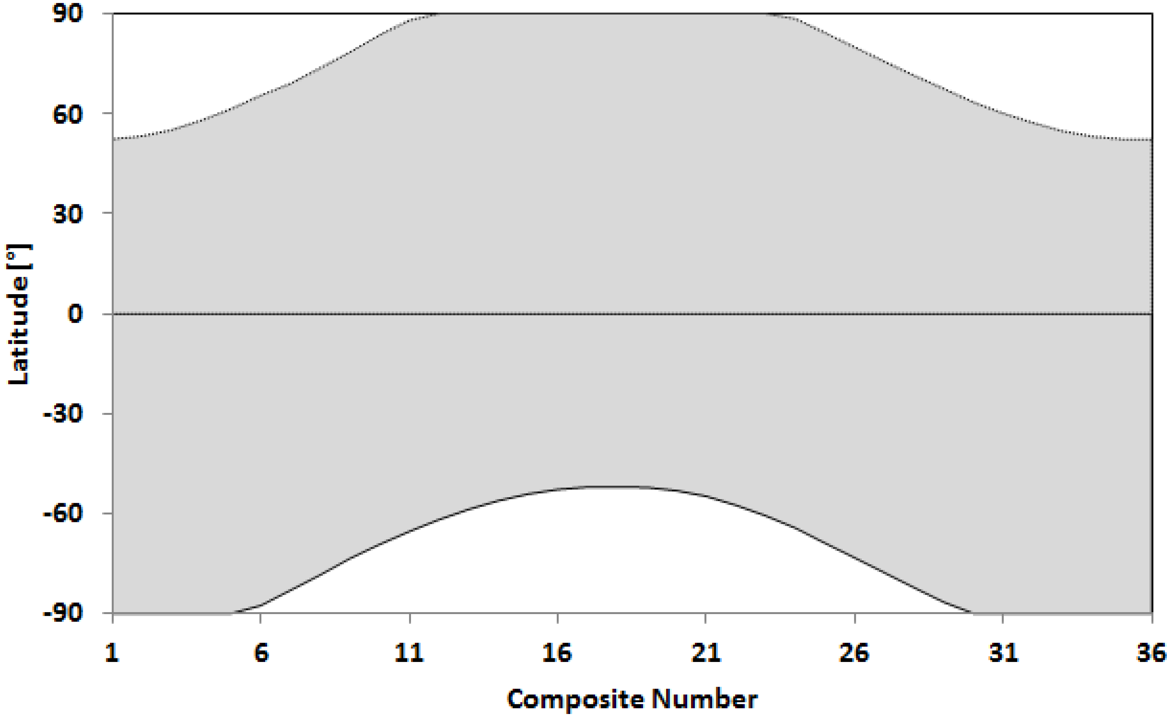
3.2.3. Adjustment of the Time Series Length

The original HA setup implies the criterion that for all grid cells, a time series with the same length needs to be approximated. However, vegetation activity is strongly dependent on the geographical location. In addition, optical remote sensing imagery, derived in unfavorable conditions, especially at too high solar zenith angles (e.g., >80°), are difficult to interpret and are likely to contain errors, because of shading effects. Since the ENVISAT MERIS acquisition time was at approximately 10 a.m. local time, we calculated for each 10-day composite the maximum and minimum latitude at which the solar zenith angle is higher than 80° at 10 a.m. (see Figure 3), following the approach of [70]. For each pixel, we checked how many possible observations were available and shortened the maximum time series length accordingly. As an example: the vegetation phase at 75°N was shortened from 36 (365 days) to 18 (184 days) composites, because observations were only possible between Composites 9 (21–31 March) and 26 (11–20 September). In this case, Composites 1–8 and 27–36 were set to LAI = 0.0.

Figure 3. Observation range (maximum and minimum latitude) for each 10-day composite at which the solar zenith angle is constantly lower than 80° at data acquisition time (10 a.m. local time).

Figure 3. Observation range (maximum and minimum latitude) for each 10-day composite at which the solar zenith angle is constantly lower than 80° at data acquisition time (10 a.m. local time).

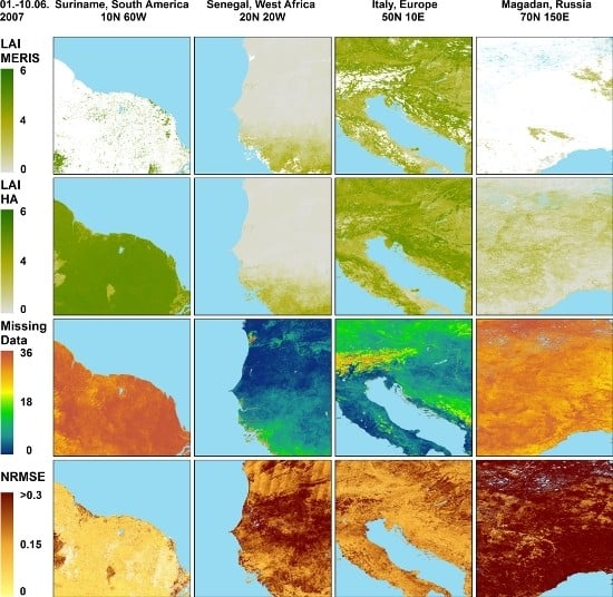
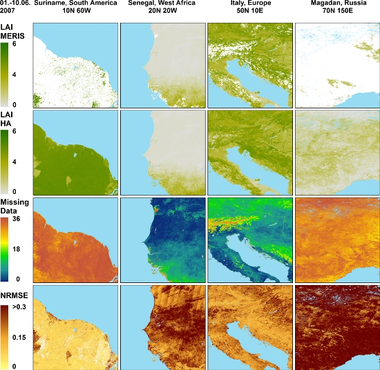
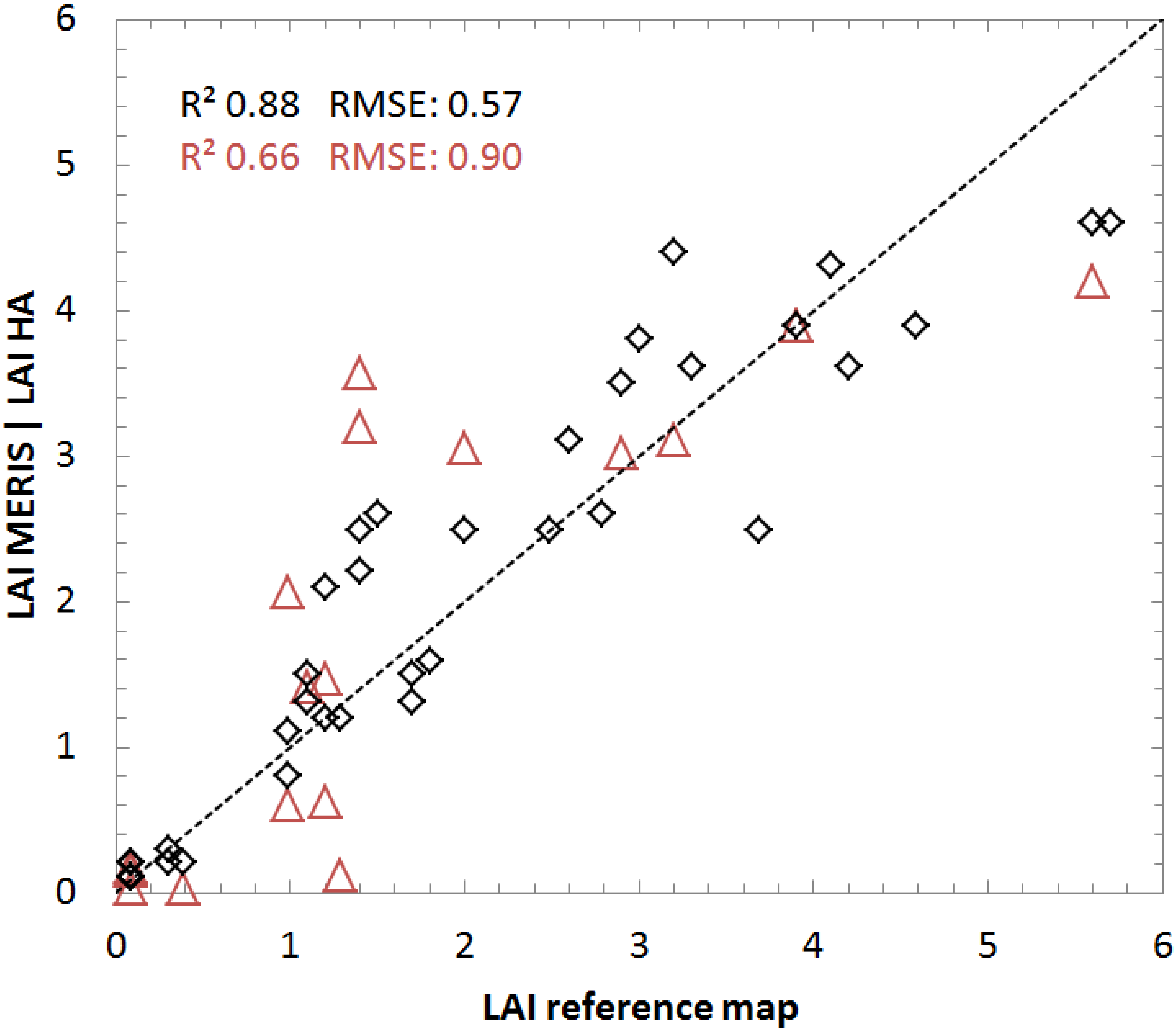
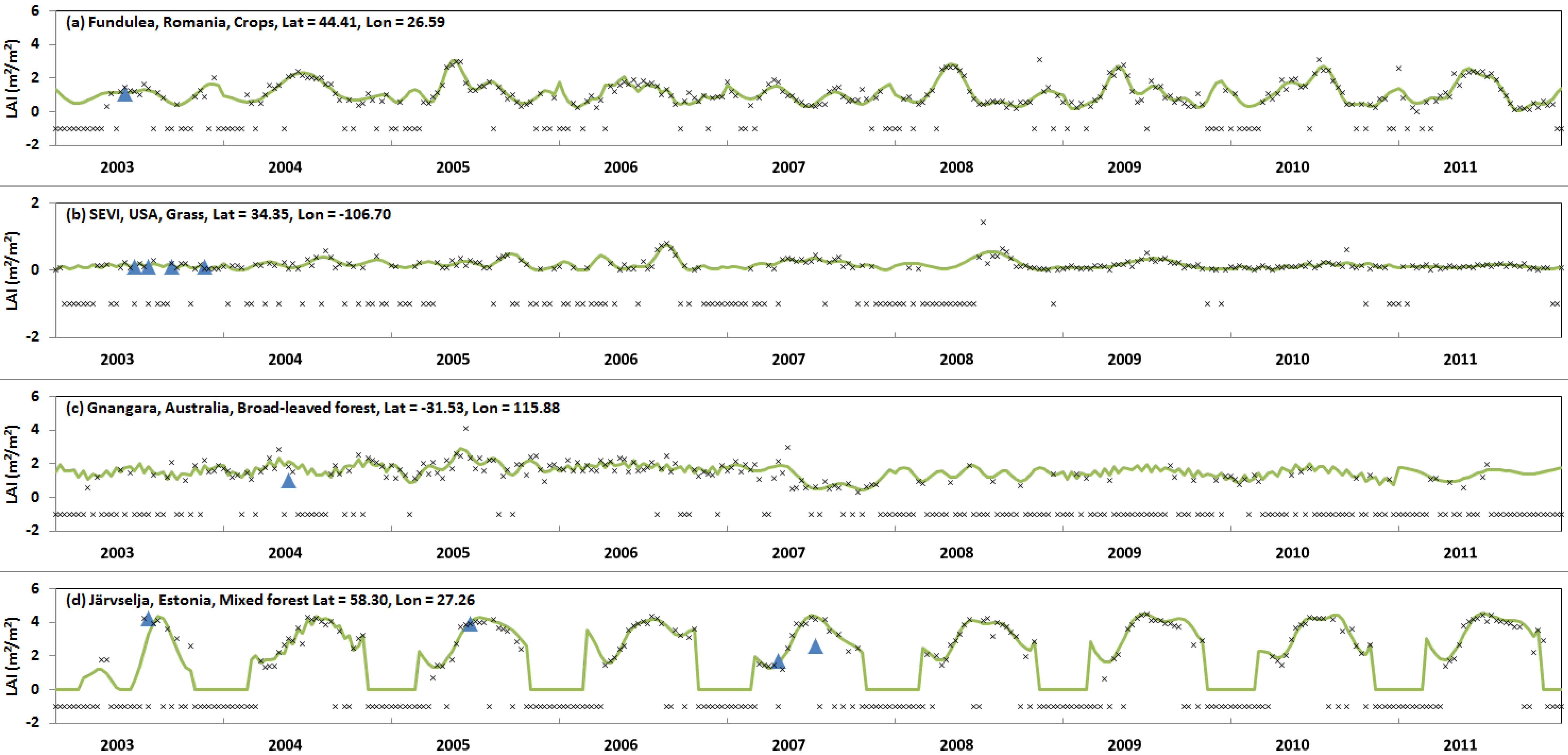
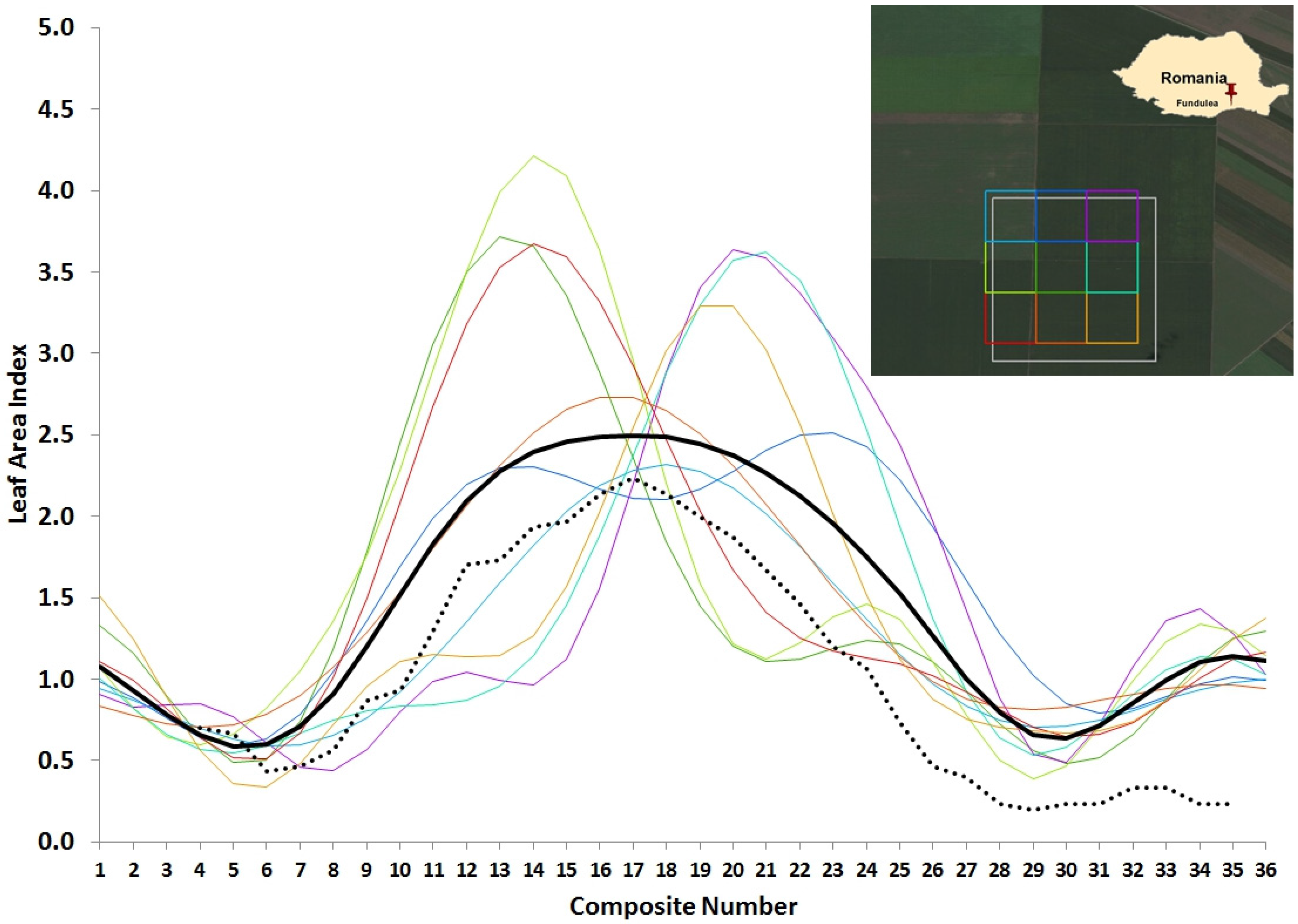
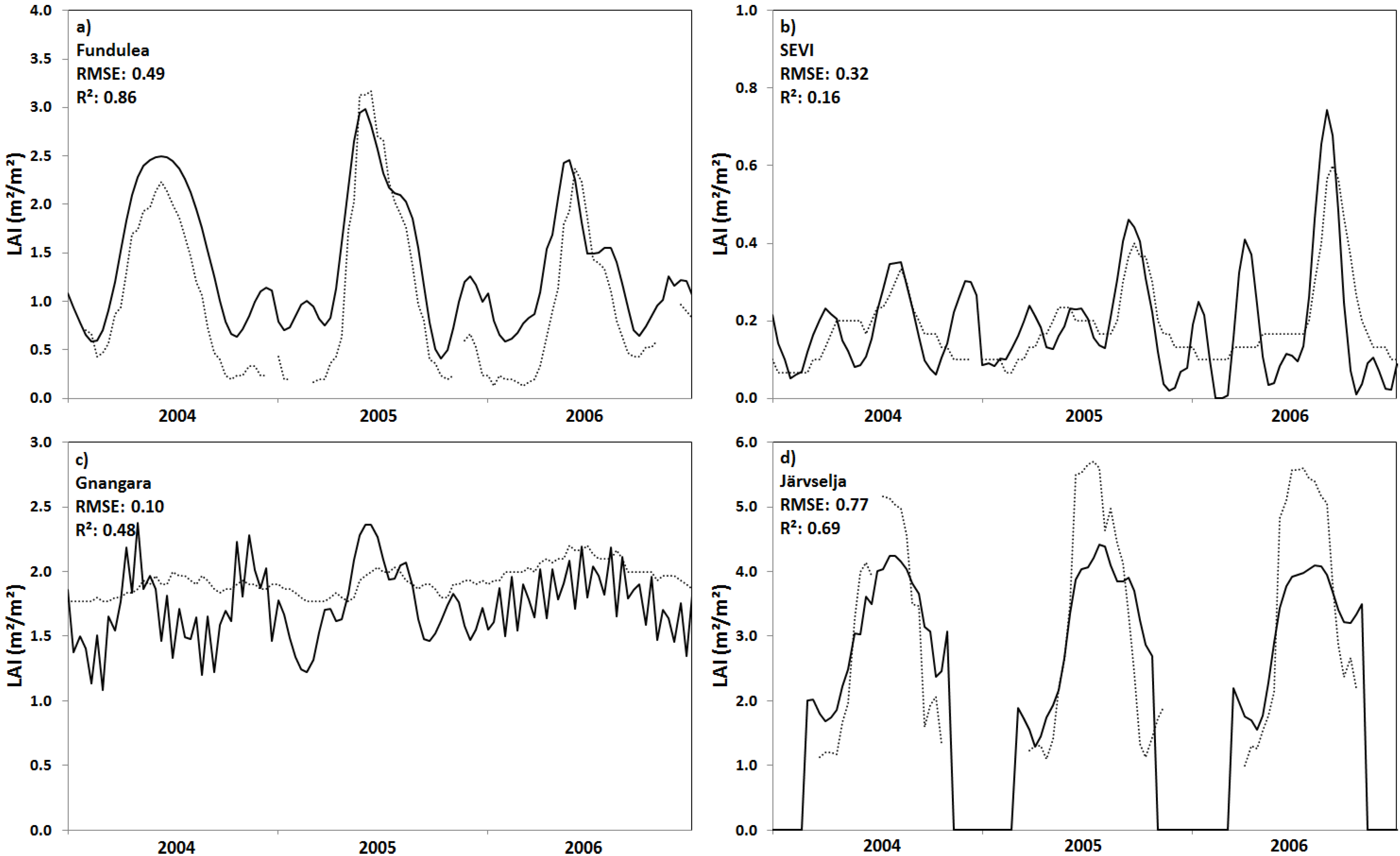
4. Exemplary Results

Four exemplary results of 10° × 10° snapshots representative for Composite 16 (1–10 July) 2007, are presented in Figure 4. The examples are chosen to show major climatic zones, like the tropics (Suriname), sub-tropics and desert (Senegal), Mediterranean (Italy) and tundra (Magadan). As can be seen, after HA is applied, all missing values (top row) are filled (second row). In order to give information on the quality of our results, Figure 4 also contains the amount of missing values per pixel (third row). As an example, the gap filling procedure for the Italy tile was applied for 29% of all pixels, from which 63% contained gaps of up to seven missing values and 12% of more than 18, which mainly occur in mountainous regions (yellow to red areas).

In the lower row of Figure 4, the normalized root mean squared error (NRMSE) is presented. It is calculated as:

$$\text{NRMSE}=\frac{\sqrt{\frac{\sum {\left({\text{LAI}}_{\text{MERIS}}-{\text{LAI}}_{\text{HA}}\right)}^2}{\mathrm{n}}}}{\overline{\text{LAI}}}$$

(2)

with $\mathrm{n}$ the number of good values and $\overline{\text{LAI}}$ the average LAI. We chose the NRMSE because it allows a better discrimination when comparing data of the same kind, but with different magnitudes. It shows a good agreement for the Suriname and Italy tile. The average NRMSE here is at 0.05 (Suriname) and 0.15 (Italy). The highest errors can be found in mountainous regions (Alps, Italy) and high latitudes (Magadan, average NRMSE: 0.60), which might be due to a combination of a lack of data and low (or no) vegetation activity. Low data availability alone, however, does not imply a bad result (see the Suriname tile), which might be due to the more homogenous landscape and, thus, a better performance when filling the gaps. Areas with highly variable meteorological conditions, such as, e.g., the Sahel (Senegal tile), show high errors. Here, precipitation is controlled by monsoon seasonality in the south and trade winds in the north [71], which imply short rain seasons with irregular events and long droughts during the rest of the year [72]. Therefore, low LAI values during the dry and high during the wet season, combined with an abrupt increase, are expected. Such single features strongly affect time series analysis and can lead to high discrepancies between the original and the processed data. A further feature that can be discovered within the NRMSE is the tracking effects (Senegal and Suriname), which are due to the particular data availability at these locations.

Figure 4. Example data of four 10° × 10° areas of the period 1–10 June 2007. Latitude/longitude values represent the top left corner of each 10° × 10° tile. Top row: MERIS 10-day composite Leaf Area Index (LAI) (0–6); second row: harmonic analysis (HA) LAI result (0–6); third row: missing data values (0–36); lower row: normalized root mean squared error (NRMSE) (0–0.3). White pixels in the top row show missing data. Blue pixels represent water.

Figure 4. Example data of four 10° × 10° areas of the period 1–10 June 2007. Latitude/longitude values represent the top left corner of each 10° × 10° tile. Top row: MERIS 10-day composite Leaf Area Index (LAI) (0–6); second row: harmonic analysis (HA) LAI result (0–6); third row: missing data values (0–36); lower row: normalized root mean squared error (NRMSE) (0–0.3). White pixels in the top row show missing data. Blue pixels represent water.

5. Results and Discussion

To assess the quality of our product, we compared it to a selected set of ground measurements (see Table 1), taken from the VALERI [73] and BigFoot [35] databases. Our approach is comparable to the approach of [41], who used VALERI ground measurements for comparison with neural network-estimated MERIS LAI.

The reference maps were produced according to the guidelines of the Land Product Validation (LPV) sub-group of the Committee Earth Observing Satellites’ Working Group on Calibration and Validation (CEOS WGCV) by extrapolation of local true LAI ground measurements to high and medium spatial resolution satellite products. For this, high spatial resolution satellite images (SPOT, ETM+, ASTER) were used and a sensor-specific transfer function applied [73] to integrated field data with high resolution imagery. In order to compare the LAI reference maps with our results, a re-projection to the WGS-84 datum was needed, which was already described by [73]. VALERI sites typically comprise an area of 3 km × 3 km. BigFoot sites are slightly larger (5 km × 5 km).

Table 1. Characteristics of selected VALERI (Validation of Land European Remote Sensing Instruments) (20) and BigFoot (2) sites. Header abbreviations: Lat, latitude; Lon, longitude; LC, land cover; ${\text{LAI}}_{\text{ref}}$, mean LAI value of the reference map; ${\text{LAI}}_{\text{MERIS}}$, LAI value of the corresponding 10-day composite at the Lat/Lon of the test site; ${\text{LAI}}_{\text{HA}}$, mean LAI value of processed MERIS data; MF, mixed forest; EBF, evergreen broad-leaved forest; ENF, evergreen needle-leaved forest. The minus symbol corresponds to a missing value. CHEQ, Chequamegon National Forest station; HARV, Harvard Forest station; NOBS, Northern Old Black Sprice station; SEVI, Sevilleta station; TUND, Tundra station.

Site	Country	Lat	Lon	LC	Date	$\mathit{L}\mathit{A}{\mathit{I}}_{\mathit{r}\mathit{e}\mathit{f}}$	$\mathit{L}\mathit{A}{\mathit{I}}_{\mathit{M}\mathit{E}\mathit{R}\mathit{I}\mathit{S}}$	$\mathit{L}\mathit{A}{\mathit{I}}_{\mathit{H}\mathit{A}}$
Alpilles	France	48.81	4.71	Crops	20 July 2002	1.7	-	1.3
Barrax	Spain	39.06	−2.10	Crops	12 July 2003	1.0	2.1	0.8
CHEQ	USA	45.95	−90.27	EBF	8 August 2002	3.0	-	3.8
Chilbolton	GB	51.10	−1.26	Crops	10 June 2006	2.9	3.0	3.5
Concepción	Chile	−37.28	−73.28	MF	9 January 2003	3.2	3.1	4.4
Counami	French Guiana	5.34	−53.24	EBF	13 October 2002	4.1	-	4.3
Demmin	Germany	53.89	13.21	Crops	23 July 2004	3.7	-	2.5
Donga	Benin	9.77	1.75	Grass	20 June 2005	1.8	-	1.6
Fundulea	Romania	44.41	26.59	Crops	24 May 2003	1.1	1.4	1.5
Gnangara	Australia	−31.53	115.88	EBF	1 March 2004	1.0	0.6	1.1
HARV	USA	42.53	−72.17	MF	24 August 2002	4.6	-	3.9
Haouz	Morocco	31.39	−7.36	Crops	12 March 2003	1.3	0.1	1.2
Hirsikangas	Finland	62.38	27.00	ENF	14 August 2003	2.5	-	2.5
					8 July 2004	1.5	-	2.6
					8 June 2005	1.4	3.2	2.5
Hyytiala	Finland	61.51	24.18	ENF	6 July 2008	2.0	3.0	2.5
Järvselja	Estonia	58.30	27.26	MF	27 July 2003	4.2	-	3.6
					29 June 2005	3.9	3.9	3.9
					22 March 2007	1.7	-	1.5
					18 August 2007	2.6	-	3.1
Laprida	Argentina	−36.59	−60.33	Grass	19 October 2002	2.8	-	2.6
Larose	Canada	45.23	−75.13	MF	7 August 2003	5.7	-	4.6
NOBS	USA	55.88	−98.48	EBF	14 July 2002	3.3	-	3.6
PlandeDieu	France	44.20	4.95	Crops	7 July 2004	1.2	0.6	1.2
Rovaniemi	Finland	66.27	25.21	ENF	9 June 2004	1.2	1.5	2.1
					15 June 2005	1.4	3.6	2.2
SEVI	USA	34.35	−106.70	Grass	26 July 2002	0.1	-	0.2
					22 August 2002	0.3	-	0.3
					9 September 2002	0.4	0.0	0.2
					15 November 2002	0.3	-	0.2
					23 June 2003	0.1	-	0.1
					28 July 2003	0.1	-	0.1
					15 September 2003	0.1	0.2	0.1
					21 November 2003	0.1	0.0	0.1
Sonian	Belgium	50.77	4.41	MF	26 June 2004	5.6	4.2	4.6
TUND	USA	71.28	−156.61	Tundra	15 August 2002	1.1	-	1.3
Turco	Bolivia	−18.24	−68.19	Grass	15 March 2003	0.1	-	0.2
Wankama	Niger	13.65	2.64	Grass	23 June 2005	0.1	0.2	0.2

Table 1. Characteristics of selected VALERI (Validation of Land European Remote Sensing Instruments) (20) and BigFoot (2) sites. Header abbreviations: Lat, latitude; Lon, longitude; LC, land cover; ${\text{LAI}}_{\text{ref}}$, mean LAI value of the reference map; ${\text{LAI}}_{\text{MERIS}}$, LAI value of the corresponding 10-day composite at the Lat/Lon of the test site; ${\text{LAI}}_{\text{HA}}$, mean LAI value of processed MERIS data; MF, mixed forest; EBF, evergreen broad-leaved forest; ENF, evergreen needle-leaved forest. The minus symbol corresponds to a missing value. CHEQ, Chequamegon National Forest station; HARV, Harvard Forest station; NOBS, Northern Old Black Sprice station; SEVI, Sevilleta station; TUND, Tundra station.

Site	Country	Lat	Lon	LC	Date	$\mathit{L}\mathit{A}{\mathit{I}}_{\mathit{r}\mathit{e}\mathit{f}}$	$\mathit{L}\mathit{A}{\mathit{I}}_{\mathit{M}\mathit{E}\mathit{R}\mathit{I}\mathit{S}}$	$\mathit{L}\mathit{A}{\mathit{I}}_{\mathit{H}\mathit{A}}$
Alpilles	France	48.81	4.71	Crops	20 July 2002	1.7	-	1.3
Barrax	Spain	39.06	−2.10	Crops	12 July 2003	1.0	2.1	0.8
CHEQ	USA	45.95	−90.27	EBF	8 August 2002	3.0	-	3.8
Chilbolton	GB	51.10	−1.26	Crops	10 June 2006	2.9	3.0	3.5
Concepción	Chile	−37.28	−73.28	MF	9 January 2003	3.2	3.1	4.4
Counami	French Guiana	5.34	−53.24	EBF	13 October 2002	4.1	-	4.3
Demmin	Germany	53.89	13.21	Crops	23 July 2004	3.7	-	2.5
Donga	Benin	9.77	1.75	Grass	20 June 2005	1.8	-	1.6
Fundulea	Romania	44.41	26.59	Crops	24 May 2003	1.1	1.4	1.5
Gnangara	Australia	−31.53	115.88	EBF	1 March 2004	1.0	0.6	1.1
HARV	USA	42.53	−72.17	MF	24 August 2002	4.6	-	3.9
Haouz	Morocco	31.39	−7.36	Crops	12 March 2003	1.3	0.1	1.2
Hirsikangas	Finland	62.38	27.00	ENF	14 August 2003	2.5	-	2.5
					8 July 2004	1.5	-	2.6
					8 June 2005	1.4	3.2	2.5
Hyytiala	Finland	61.51	24.18	ENF	6 July 2008	2.0	3.0	2.5
Järvselja	Estonia	58.30	27.26	MF	27 July 2003	4.2	-	3.6
					29 June 2005	3.9	3.9	3.9
					22 March 2007	1.7	-	1.5
					18 August 2007	2.6	-	3.1
Laprida	Argentina	−36.59	−60.33	Grass	19 October 2002	2.8	-	2.6
Larose	Canada	45.23	−75.13	MF	7 August 2003	5.7	-	4.6
NOBS	USA	55.88	−98.48	EBF	14 July 2002	3.3	-	3.6
PlandeDieu	France	44.20	4.95	Crops	7 July 2004	1.2	0.6	1.2
Rovaniemi	Finland	66.27	25.21	ENF	9 June 2004	1.2	1.5	2.1
					15 June 2005	1.4	3.6	2.2
SEVI	USA	34.35	−106.70	Grass	26 July 2002	0.1	-	0.2
					22 August 2002	0.3	-	0.3
					9 September 2002	0.4	0.0	0.2
					15 November 2002	0.3	-	0.2
					23 June 2003	0.1	-	0.1
					28 July 2003	0.1	-	0.1
					15 September 2003	0.1	0.2	0.1
					21 November 2003	0.1	0.0	0.1
Sonian	Belgium	50.77	4.41	MF	26 June 2004	5.6	4.2	4.6
TUND	USA	71.28	−156.61	Tundra	15 August 2002	1.1	-	1.3
Turco	Bolivia	−18.24	−68.19	Grass	15 March 2003	0.1	-	0.2
Wankama	Niger	13.65	2.64	Grass	23 June 2005	0.1	0.2	0.2

For the quality assessment, we only used LAI reference map pixels, which overly the corresponding MERIS pixels by more than 70%. To reduce errors resulting from the re-projection and possible delocalization uncertainties, we calculated the mean value of all pixels, referred to as ${\text{LAI}}_{\text{ref}}$ (reference map) and ${\text{LAI}}_{\text{HA}}$ (our result) in Table 1. In addition, the MERIS values of the corresponding 10-day composite are presented $({\text{LAI}}_{\text{MERIS}})$. For the assessment, a total of 38 LAI values from 25 sites worldwide were analyzed. The land cover types of these sites range from evergreen broad-leaved forest (EBF), to evergreen needle-leaved forest (ENF), mixed forest (MF), crops and grassland. The scatterplot of this comparison is presented in Figure 5, which shows a good overall result (R²: 0.88; RMSE: 0.57). In contrast, when comparing the original MERIS LAI data with the BigFoot/VALERI sites, an R² of only 0.66 (RMSE: 0.90) can be found. The increased accuracy might be due to, e.g., the outlier detection process that was applied.

Figure 5. Validation of time series-analyzed MERIS data with VALERI and BigFoot measurements. Red triangles represent the comparison of Leaf Area Index (LAI) MERIS with LAI reference maps. Black diamonds represent the comparison of LAI harmonic analysis (HA) with LAI reference maps.

Figure 5. Validation of time series-analyzed MERIS data with VALERI and BigFoot measurements. Red triangles represent the comparison of Leaf Area Index (LAI) MERIS with LAI reference maps. Black diamonds represent the comparison of LAI harmonic analysis (HA) with LAI reference maps.

The RMSE of our correlation of ground measurements with neural network-estimated MERIS LAI is in close agreement with the findings of [41] (RMSE = 0.47).

Figure 6. Temporal development of the original MERIS (black crosses), processed (green solid line) and BigFoot/VALERI (blue Triangles) data for the period 2003–2011, for: (a) Fundulea (crops); (b) SEVI (grass); (c) Gnangara (broad-leaved forest); (d) Järvselja (mixed forest). Negative values (−1) represent missing observations.

Figure 6. Temporal development of the original MERIS (black crosses), processed (green solid line) and BigFoot/VALERI (blue Triangles) data for the period 2003–2011, for: (a) Fundulea (crops); (b) SEVI (grass); (c) Gnangara (broad-leaved forest); (d) Järvselja (mixed forest). Negative values (−1) represent missing observations.

To assess the quality of the temporal fit of the HA, we investigated the LAI development of the period 2003–2011, as shown in Figure 6, for selected main land cover types (crops, grass, broad-leaved and mixed forest). As can be seen, the processed time series provide a smoothed fit to the MERIS data. They also show an acceptable agreement with most of the LAI reference map values. However, for the Gnangara site and the mid-2007 value of Järvselja, significant differences are observed. The general accordance is comparable to the findings of [47], who observed partially high differences of reference map values to original and improved MODIS LAI data. The original data of the Gnangara site shows, for the first five years, short-term fluctuations, which might not be representative for natural development of broad-leaved forests. However, the HA results here show features of these fluctuations. Since the data availability for this site is significantly worse from 2008 onwards, the HA results should be regarded with caution. A reason for the low data availability can be found in changes within the prioritization at the three ground stations that received MERIS over Australia (Alice Springs, Hobart and Parepare). This is opposite the desert grassland test site SEVI (Sevilleta, NM, USA), where data availability significantly improved in mid-2008. The reason for this is the start of MERIS data acquisition at two Canada Centre for Remote Sensing (CCRS) stations from May 2008 onwards covering Canada and the USA. The Järvselja plot shows, due to its high latitude and the HA setup as described above, a shorter vegetation period of only 25 10-day composites. Some artifacts, like the high start LAI values in 2006, 2009 and 2011, are still visible. A reason could be that even with the shortened vegetation period, the variation was not captured properly.

In order to visualize the information content of our MERIS LAI product, we selected the agricultural site of Fundulea and did a comparison of our product with the Geoland2 LAI product, according to [34] the most accurate LAI dataset for agriculture. We chose this site, because its land use is described as cropland, and thus, it is most likely to find time series triggered by agricultural management within a small area. In Figure 7, we present an exemplary comparison for this site for 2004. Approximately 10.2 MERIS pixels cover the same pixel area of one SPOT pixel. For our comparison, we only used the nine MERIS pixels, which lay with at least 80% within the bounding box of the VGT pixel. From Figure 7, it can be seen that the SPOT pixel covers more than one agricultural field (see the RGB background image). No prominent peaks in the early or late vegetative phase can be discovered, which would be expected on a managed agricultural site. The nine MERIS LAI time series (colored lines) show a considerably different behavior, with typical peaks in the early or late vegetation phase depending on the agricultural management (summer or winter crops). The average MERIS LAI time series of all nine pixels (bold black line in Figure 7), however, shows a highly comparable pattern as the VGT-LAI time series (dotted black line). The comparison of spatially-averaged MERIS LAI time series with VGT-LAI time series for selected BigFoot/VALERI sites, covering all dominant landscape ecosystems, confirmed the finding of Figure 7. This comparison gives a first impression about the comparability of our averaged MERIS LAI dataset to existing LAI products, such as, e.g. VGT-LAI and MODIS LAI. However, the more than nine-times higher spatial resolution of our MERIS LAI time series contains more detailed spatial and temporal information, especially for highly heterogeneous areas. This is especially important and helpful for studies in, e.g., agricultural areas and for investigating land use change.

Figure 7. Leaf Area Index inter-comparison of nine MERIS-LAI-HA and the corresponding Geoland2-SPOT-VGT-LAI at the Fundulea, Romania (crops), site for 2004. Top right: RGB image (Google Earth) of the Fundulea area with: grey rectangles, SPOT 1 km × 1 km pixel; colored rectangles, MERIS pixels. Graph: each colored line corresponds to the rectangle with the same color. Bold black line, average LAI of all nine colored LAI lines; dashed line, SPOT-VEGETATION LAI.

Figure 7. Leaf Area Index inter-comparison of nine MERIS-LAI-HA and the corresponding Geoland2-SPOT-VGT-LAI at the Fundulea, Romania (crops), site for 2004. Top right: RGB image (Google Earth) of the Fundulea area with: grey rectangles, SPOT 1 km × 1 km pixel; colored rectangles, MERIS pixels. Graph: each colored line corresponds to the rectangle with the same color. Bold black line, average LAI of all nine colored LAI lines; dashed line, SPOT-VEGETATION LAI.

Finally, we performed an inter-comparison between Geoland2 LAI products based on 1 km SPOT-VGT data and our new MERIS-FR-LAI products for the four test sites shown in Figure 6. We resampled the MERIS-FR-LAI product by averaging nine MERIS-FR pixels, which corresponds to the SPOT-VGT pixel. An exemplary result for the period 2004–2006 for the four sites, Fundulea, SEVI, Gnangara and Järvselja, is presented in Figure 8. It can be seen that for all four sites, both LAIs follow similar temporal trajectories. The strongest agreement (R²: 0.86) can be found for the agricultural site Fundulea (Figure 8a; also see Figure 7), followed by the mixed forest site (Järvselja; Figure 8d). However, for the mixed forest site, the temporal LAI profiles show differences in their magnitude, which result in an increased RMSE (0.77). For the evergreen broad-leaved forest site (Gnangara; Figure 8c), our gap-filling and smoothing approach (harmonic analysis) results in small amplitude (±0.1), but high frequency oscillations, when a close to constant LAI is approximated. This results in a low R² of only 0.48, but combined with the very small RMSE of 0.10, the overall agreement is still given. For the desert grassland/shrub land site (SEVI; Figure 8b), the agreement between SPOT-VGT LAI and the MERIS-LAI is low (R²: 0.16). The SEVI site consists largely of perennial bunchgrass, with small amounts of cacti and shrubs. However, this finding is due to very low LAIs (<0.5) for most estimates of the time series. Historic field measurements [35] also published low LAI measurements demonstrating that the relative standard deviation of LAI field measurements in the SEVI area can be up to 60%. This is confirmed by [74], who showed large discrepancies between different ground-based LAI measurements for heterogeneous and short crop canopies due to the substantial differences in the spatial sampling of transmittance (up to RMSE of 0.16). For shrub and grass land, at least the same error for the LAI measurements is expected, as well as for remote sensing-derived LAI products. Overall, the MERIS-FR LAI pattern generally follows the Geoland2-SPOT-VEGETATION-based LAI time series for all test sites.

Figure 8. Data inter-comparison of Geoland2 (dotted line) and MERIS-HA (black line) LAI time series for the four sites, (a) Fundulea; (b) SEVI; (c) Gnangara and (d) Järvselja, for three exemplary years (2004–2006).

Figure 8. Data inter-comparison of Geoland2 (dotted line) and MERIS-HA (black line) LAI time series for the four sites, (a) Fundulea; (b) SEVI; (c) Gnangara and (d) Järvselja, for three exemplary years (2004–2006).

6. Conclusions

The complete Level 1B MERIS-FR archive has been reprocessed to derive global continuous 10-day composites of LAI for the period July 2002–March 2012. Cloud contamination, topographic effects and restriction to the solar zenith angle were identified as sources for missing data and outliers within the time series. We applied time series analysis to improve the dataset and successfully filled gaps with reliable data. This was mainly done because remote sensing-driven vegetation models, such as e.g., the Biosphere Energy Transfer Hydrology (BETHY/DLR) model [75], operated at German Aerospace Center (DLR), strongly rely on such gap-free datasets.

We used an adjusted version of the HA to derive continuous, gap-free time series. HA was originally developed to process time series of ozone information in the stratosphere. The adjustment includes the development of a single and multi-year phenological mean, outlier detection and an adjustment of the vegetation phase. Validation has been performed using LAI reference maps from the BigFoot and VALERI databases, which show good congruence and a high coefficient of determination (R² = 0.88). The normalized RMSE has been calculated for selected regions and also shows a good agreement, except in mountainous regions or at high latitudes.

Next to the reprocessed MODIS LAI product introduced by [47] and the GLASS (Global Land Surface Satellites) by [16], which also claims to be spatiotemporally continuous, this is the first globally-available gap-free dataset with less than a 1-km² resolution and the first global MERIS-FR LAI dataset covering the full time of ENVISAT MERIS operation (2002–2012). Spatiotemporal continuous datasets, such as developed and described here, are applicable for global or regional vegetation models where LAI data are often used as a proxy to describe phenology. In principle, our method is adaptable to LAI time series with comparable resolutions. We already processed the Geoland2 LAI database, which is based on SPOT-VGT data, and found similar results. We thus believe our method to be applicable to phenological time series derived with different sensors, such as, e.g., Proba-V, Terra/Aqua-MODIS, as well as the prospective Sentinel 3-OLCI (Ocean and Land Colour Instrument). The dataset as described in this paper can be accessed at [76].

References

1. Cayrol, P.; Kergoat, L.; Moulin, S.; Dedieu, G.; Chehbouni, A. Calibrating a coupled SVAT–vegetation growth model with remotely sensed reflectance and surface temperature—A case study for the HAPEX-sahel grassland sites. J. Appl. Meteorol. 2000, 39, 2452–2472. [Google Scholar] [CrossRef]
2. Tucker, C.J.; Sellers, P.J. Satellite remote sensing of primary production. Int. J. Remote Sens. 1986, 7, 1395–1416. [Google Scholar] [CrossRef]
3. Sellers, P.J.; Berry, J.A.; Collatz, G.J.; Field, C.B.; Hall, F.G. Canopy reflectance, photosynthesis, and transpiration. III. A reanalysis using improved leaf models and a new canopy integration scheme. Remote Sens. Environ. 1992, 42, 187–216. [Google Scholar] [CrossRef]
4. Myneni, R.B.; Hall, F.G.; Sellers, P.J.; Marshak, A.L. The interpretation of spectral vegetation indexes. IEEE Trans. Geosci. Remote Sens. 1995, 33, 481–486. [Google Scholar] [CrossRef]
5. Sellers, P.J. Canopy reflectance, photosynthesis and transpiration. Int. J. Remote Sens. 1985, 6, 1335–1372. [Google Scholar] [CrossRef]
6. Los, S.O.; Justice, C.O.; Tucker, C.J. A global 1° by 1° NDVI data set for climate studies derived from the GIMMS continental NDVI data. Int. J. Remote Sens. 1994, 15, 3493–3518. [Google Scholar] [CrossRef]
7. Sellers, P.J.; Tucker, C.J.; Collatz, G.J.; Los, S.O.; Justice, C.O.; Dazlich, D.; Randall, D.A. A global 1° by 1° NDVI data set for climate studies. Part 2: The generation of global fields of terrestrial biophysical parameters from the NDVI. Int. J. Remote Sens. 2007, 15, 3519–3545. [Google Scholar] [CrossRef]
8. Poulter, B.; Pederson, N.; Liu, H.; Zhu, Z.; D’Arrigo, R.; Ciais, P.; Davi, N.; Frank, D.; Leland, C.; Myneni, R.B.; et al. Recent trends in Inner Asian forest dynamics to temperature and precipitation indicate high sensitivity to climate change. Agric. For. Meteorol. 2013, 178–179, 31–45. [Google Scholar] [CrossRef]
9. Zhu, Z.; Bi, J.; Pan, Y.; Ganguly, S.; Anav, A.; Xu, L.; Samanta, A.; Piao, S.; Nemani, R.R.; Myneni, R.B. Global data sets of vegetation leaf area index (LAI)3g and fraction of photosynthetically active radiation (FPAR)3g derived from global inventory modeling and mapping studies (GIMMS) normalized difference vegetation index (NDVI3g) for the period 1981 to 2011. Remote Sens. 2013, 5, 927–948. [Google Scholar]
10. Fang, H.; Jiang, C.; Li, W.; Wei, S.; Baret, F.; Chen, J.M.; Garcia-Haro, J.; Liang, S.; Liu, R.; Myneni, R.B.; et al. Characterization and intercomparison of global moderate resolution leaf area index (LAI) products: Analysis of climatologies and theoretical uncertainties. J. Geophys. Res. Biogeosci. 2013, 118, 529–548. [Google Scholar] [CrossRef]
11. Gao, F.; Morisette, J.T.; Wolfe, R.E.; Ederer, G.; Pedelty, J.; Masuoka, E.; Myneni, R.B.; Tan, B.; Nightingale, J. An algorithm to produce temporally and spatially continuous MODIS-LAI time series. IEEE Geosci. Remote Sens. Lett. 2008, 5, 60–64. [Google Scholar] [CrossRef]
12. Myneni, R.B.; Hoffman, S.; Privette, J.L.; Glassy, J.; Tian, Y.; Wang, Y.; Song, X.; Zhang, Y.; Smith, G.R.; Lotsch, A.; et al. Global products of vegetation leaf area and fraction absorbed PAR from year one of MODIS data. Remote Sens. Environ. 2002, 83, 214–231. [Google Scholar] [CrossRef]
13. Baret, F.; Weiss, M.; Lacaze, R.; Camacho, F.; Makhmara, H.; Pacholcyzk, P.; Smets, B. GEOV1: LAI and FAPAR essential climate variables and FCOVER global time series capitalizing over existing products. Part1: Principles of development and production. Remote Sens. Environ. 2013, 137, 299–309. [Google Scholar] [CrossRef]
14. Baret, F.; Hagolle, O.; Geiger, B.; Bicheron, P.; Miras, B.; Huc, M.; Berthelot, B.; Niño, F.; Weiss, M.; Samain, O.; et al. LAI, fAPAR and fCover CYCLOPES global products derived from VEGETATION. Remote Sens. Environ. 2007, 110, 275–286. [Google Scholar] [CrossRef] [Green Version]
15. Verger, A.; Baret, F.; Weiss, M. A multisensor fusion approach to improve LAI time series. Remote Sens. Environ. 2011, 115, 2460–2470. [Google Scholar] [CrossRef]
16. Xiao, Z.; Liang, S.; Wang, J.; Chen, P.; Yin, X.; Zhang, L.; Song, J. Use of general regression neural networks for generating the GLASS leaf area index product from time-series MODIS surface reflectance. IEEE Trans. Geosci. Remote Sens. 2014, 52, 209–223. [Google Scholar] [CrossRef]
17. Liu, Y.; Liu, R.; Chen, J.M. Retrospective retrieval of long-term consistent global leaf area index (1981–2011) from combined AVHRR and MODIS data. J. Geophys. Res. 2012, 117. [Google Scholar] [CrossRef]
18. Pinty, B.; Andredakis, I.; Clerici, M.; Kaminski, T.; Taberner, M.; Verstraete, M.M.; Gobron, N.; Plummer, S.; Widlowski, J.-L. Exploiting the MODIS albedos with the two-stream inversion package (JRC-TIP): 1. Effective leaf area index, vegetation, and soil properties. J. Geophys. Res. 2011, 116, 1–20. [Google Scholar] [CrossRef]
19. Nemani, R.R.; Keeling, C.D.; Hashimoto, H.; Jolly, W.M.; Piper, S.C.; Tucker, C.J.; Myneni, R.B.; Running, S.W. Climate-driven increases in global terrestrial net primary production from 1982 to 1999. Science 2003, 300, 1560–1563. [Google Scholar] [CrossRef] [PubMed]
20. Tesemma, Z.K.; Wei, Y.; Western, A.W.; Peel, M.C. Leaf area index variation for crop, pasture, and tree in response to climatic variation in the Goulburn–Broken catchment, Australia. J. Hydrometeor. 2014, 15, 1592–1606. [Google Scholar] [CrossRef]
21. Turner, D.P.; Cohen, W.B.; Kennedy, R.E.; Fassnacht, K.S.; Briggs, J.M. Relationships between leaf area index and Landsat TM spectral vegetation indices across three temperate zone sites. Remote Sens. Environ. 1999, 70, 52–68. [Google Scholar] [CrossRef]
22. Running, S.W.; Baldocchi, D.D.; Turner, D.P.; Gower, S.T.; Bakwin, P.S.; Hibbard, K.A. A global terrestrial monitoring network integrating tower fluxes, flask sampling, ecosystem modeling and EOS satellite data. Remote Sens. Environ. 1999, 70, 108–127. [Google Scholar] [CrossRef]
23. Alton, P.B. From site-level to global simulation: Reconciling carbon, water and energy fluxes over different spatial scales using a process-based ecophysiological land-surface model. Agric. For. Meteorol. 2013, 176, 111–124. [Google Scholar] [CrossRef]
24. Tum, M.; Günther, K.P.; McCallum, I.; Kindermann, G.; Schmid, E. Sustainable bioenergy potentials for Europe and the globe. Geoinf. Geo. Over. 2013, S1, 1–7. [Google Scholar]
25. Dickinson, R.E. Land processes in climate models. Remote Sens. Environ. 1995, 51, 27–38. [Google Scholar] [CrossRef]
26. Sellers, P.J.; Dickinson, R.E.; Randall, A.K.; Hall, F.G.; Berry, J.A.; Collatz, G.J.; Denning, A.S.; Mooney, H.A.; Nobre, C.A.; Sato, N.; et al. Modeling the exchanges of energy, water, and carbon between continents and the atmosphere. Science 1997, 275, 502–509. [Google Scholar] [CrossRef] [PubMed]
27. Zhang, C.; Wang, D.; Wang, G.; Yang, W.; Liu, X. Regional differences in hydrological response to canopy interception schemes in a land surface model. Hydrol. Process. 2014, 28, 2499–2508. [Google Scholar] [CrossRef]
28. Gobron, N.; Verstraete, M.M. Assessment of the Status of the Development of the Standards for the Terrestrial Essential Climate Variables: Leaf Area Index (LAI): Version 10; GTOS: Rome, Italy, 2009. [Google Scholar]
29. Rüdiger, C.; Albergel, C.; Mahfouf, J.-F.; Calvet, J.-C.; Walker, J.P. Evaluation of the observation operator Jacobian for leaf area index data assimilation with an extended Kalman filter. J. Geophys. Res. 2010, 115, 1–10. [Google Scholar] [CrossRef]
30. Barbu, A.L.; Calvet, J.-C.; Mahfouf, J.-F.; Albergel, C.; Lafont, S. Assimilation of Soil wetness index and leaf area index into the ISBA-A-gs land surface model: Grassland case study. Biogeosciences 2011, 8, 1971–1986. [Google Scholar] [CrossRef]
31. Sabater, J.M.; Rüdiger, C.; Calvet, J.-C.; Fritz, N.; Jarlan, L.; Kerr, Y. Joint assimilation of surface soil moisture and LAI observations into a land surface model. Agric. For. Meteorol. 2008, 148, 1362–1373. [Google Scholar] [CrossRef] [Green Version]
32. Jarlan, L.; Balsamo, G.; Lafont, S.; Beljaars, A.; Calvet, J.-C.; Mougin, E. Analysis of leaf area index in the ECMWF land surface model and impact on latent heat and carbon fluxes: Application to West Africa. J. Geophys. Res. 2008, 113, 1–22. [Google Scholar] [CrossRef]
33. Weiss, M.; Baret, F.; Garrigues, S.; Lacaze, R. LAI and fAPAR CYCLOPES global products derived from VEGETATION. Part 2: Validation and comparison with MODIS collection 4 products. Remote Sens. Environ. 2007, 110, 317–331. [Google Scholar] [CrossRef]
34. Garrigues, S.; Lacaze, R.; Baret, F.; Morisette, J.T.; Weiss, M.; Nickeson, J.E.; Fernandes, R.A.; Plummer, S.E.; Myneni, R.B.; Yang, W. Validation and intercomparison of global Leaf Area Index products derived from remote sensing data. J. Geophys. Res. 2008, 113, 1–20. [Google Scholar] [CrossRef]
35. Cohen, W.B.; Maiersperger, T.K.; Pflugmacher, D. BigFoot Leaf Area Index Surfaces for North and South American Sites, 2000–2003, Data Set; Oak Ridge National Laboratory Distributed Active Archive Center: Oak Ridge, TN, USA, 2006. Available online: http://www.daac.ornl.gov (accessed on 12 January 2016).
36. VAlidation of Land European Remote Sensing Instruments (VALERI). Available online: http://w3.avignon.inra.fr/valeri/ (accessed on 8 January 2016).
37. Fernandes, R.A.; Plummer, S.E.; Nightingale, J.; Baret, F.; Camacho, F.; Fang, H.; Garrigues, S.; Gobron, N.; Lang, M.; Lacaze, R.; et al. Global leaf area index product validation good practices. In Best Practice for Satellite-Derived Land Product Validation, Land Product Validation Subgroup (WGCV/CEOS), version 2.0.; Schaepman-Strub, G., Román, M.O., Nickeson, J.E., Eds.; CEOS: Zurich, Switzerland, 2014; pp. 1–78. [Google Scholar]
38. Baret, F.; Morisette, J.T.; Fernandes, R.A.; Champeaux, J.L.; Myneni, R.B.; Chen, J.; Plummer, S.E.; Weiss, M.; Garrigues, S.; Nickeson, J.E. Evaluation of the representativeness of networks of sites for the global validation and intercomparison of land biophysical products: Proposition of the CEOS-BELMANIP. IEEE Trans. Geosci. Remote Sens. 2006, 44, 1794–1803. [Google Scholar] [CrossRef]
39. Roumenina, E.; Dimitrov, P.; Filchev, L.; Jelev, G. Validation of MERIS LAI and FAPAR products for winter wheat-sown test fields in North-East Bulgaria. Int. J. Remote Sens. 2014, 35, 3859–3874. [Google Scholar] [CrossRef]
40. Dente, L.; Satalino, G.; Mattia, F.; Rinaldi, M. Assimilation of leaf area index derived from ASAR and MERIS data into CERES-Wheat model to map wheat yield. Remote Sens. Environ. 2008, 112, 1395–1407. [Google Scholar] [CrossRef]
41. Bacour, C.; Baret, F.; Béal, D.; Weiss, M.; Pavageau, K. Neural network estimation of LAI, fAPAR, fCover and LAI×Cab, from top of canopy MERIS reflectance data: Principles and validation. Remote Sens. Environ. 2006, 105, 313–325. [Google Scholar] [CrossRef]
42. Canisius, F.; Fernandes, R.A.; Chen, J. Comparison and evaluation of Medium Resolution Imaging Spectrometer leaf area index products across a range of land use. Remote Sens. Environ. 2010, 114, 950–960. [Google Scholar] [CrossRef]
43. Dilmaghani, S.; Henry, I.C.; Soonthornnonda, P.; Christensen, E.R.; Henry, R.C. Harmonic analysis of environmental time series with missing data or irregular sample spacing. Environ. Sci. Technol. 2007, 41, 7030–7038. [Google Scholar] [CrossRef] [PubMed]
44. Scargle, J.D. Studies in astronomical time series analysis. I—Modeling random processes in the time domain. Astrophys. J. Suppl. Ser. 1981, 45, 1–71. [Google Scholar] [CrossRef]
45. Lomb, N.R. Least-squares frequency analysis of unequally spaced data. Astrophys. Space Sci. 1976, 39, 447–462. [Google Scholar] [CrossRef]
46. Jönsson, P.; Eklundh, L. TIMESAT—A program for analyzing time-series of satellite sensor data. Comput. Geosci. 2004, 30, 833–845. [Google Scholar] [CrossRef]
47. Yuan, H.; Dai, Y.; Xiao, Z.; Ji, D.; Wei, S.G. Reprocessing the MODIS Leaf Area Index products for land surface and climate modelling. Remote Sens. Environ. 2011, 115, 1171–1187. [Google Scholar] [CrossRef]
48. Chen, J.; Jönsson, P.; Tamura, M.; Gu, Z.; Matsushita, B.; Eklundh, L. A simple method for reconstructing a high-quality NDVI time-series data set based on the Savitzky–Golay filter. Remote Sens. Environ. 2004, 91, 332–344. [Google Scholar] [CrossRef]
49. Kandasamy, S.; Baret, F.; Verger, A.; Neveux, P.; Weiss, M. A comparison of methods for smoothing and gap filling time series of remote sensing observations—Application to MODIS LAI products. Biogeosciences 2013, 10, 4055–4071. [Google Scholar] [CrossRef]
50. Roerink, G.J.; Menenti, M.; Verhoef, W. Reconstructing cloudfree NDVI composites using Fourier analysis of time series. Int. J. Remote Sens. 2000, 21, 1911–1917. [Google Scholar] [CrossRef]
51. Colditz, R.R.; Conrad, C.; Wehrmann, T.; Schmidt, M.; Dech, S.W. TiSeG: A flexible software tool for time-series generation of MODIS data utilizing the quality assessment science data set. IEEE Trans. Geosci. Remote Sens. 2008, 46, 3296–3308. [Google Scholar] [CrossRef]
52. Moffat, A.M.; Papale, D.; Reichstein, M.; Hollinger, D.Y.; Richardson, A.D.; Barr, A.G.; Beckstein, C.; Braswell, B.H.; Churkina, G.; Desai, A.R.; et al. Comprehensive comparison of gap-filling techniques for eddy covariance net carbon fluxes. Agric. For. Meteorol. 2007, 147, 209–232. [Google Scholar] [CrossRef]
53. Hird, J.N.; McDermid, G.J. Noise reduction of NDVI time series: An empirical comparison of selected techniques. Remote Sens. Environ. 2009, 113, 248–258. [Google Scholar] [CrossRef]
54. Musial, J.P.; Verstraete, M.M.; Gobron, N. Technical note: Comparing the effectiveness of recent algorithms to fill and smooth incomplete and noisy time series. Atmos. Chem. Phys. 2011, 11, 7905–7923. [Google Scholar] [CrossRef] [Green Version]
55. Fang, H.; Liang, S.; Townshend, J.R.G.; Dickinson, R.E. Spatially and temporally continuous LAI data sets based on an integrated filtering method: Examples from North America. Remote Sens. Environ. 2008, 112, 75–93. [Google Scholar] [CrossRef]
56. Bittner, M.; Offermann, D.; Bugaeva, I.V.; Kokin, G.A.; Koshelkov, J.P.; Krivolutsky, A.; Tarasenko, D.A.; Gil-Ojeda, M.; Hauchecorne, A.; Lübken, F.-J.; et al. Long period/large scale oscillations of temperature during the DYANA campaign. J. Atmos. Terr. Phys. 1994, 56, 1675–1700. [Google Scholar] [CrossRef]
57. Meisner, R.E.; Bittner, M.; Dech, S.W. Computer animation of remote sensing-based time series data sets. IEEE Trans. Geosci. Remote Sens. 1999, 37, 1100–1106. [Google Scholar] [CrossRef]
58. Erbertseder, T.; Eyring, V.; Bittner, M.; Dameris, M.; Grewe, V. Hemispheric ozone variability indices derived from satellite observations and comparison to a coupled chemistry-climate model. Atmos. Chem. Phys. 2006, 6, 5105–5120. [Google Scholar] [CrossRef]
59. European Space Agency (ESA). Envisat MERIS FRS Density Maps. 2014. Available online: https://earth.esa.int/web/guest/-/envisat-meris-frs-density-maps (accessed on 7 January 2016).
60. ACRI-ST. AMORGOS (Accurate MERIS Ortho-Rectified Geo-Location Operational Software) Versions 3.0 and 4.0. 2012. Available online: https://earth.esa.int/web/guest/-/amorgos-40p1–4410 (accessed on 7 January 2016).
61. Muller, J.-P.; López, G.; Potts, D.; Shane, N.; Kharbouche, S.; Fisher, D.; Lewis, P.; Brockmann, C.; Danne, O.; Krüger, O.; et al. GlobAlbedo: Theoretical Basis Document V4_12; London’s Global University: London, UK, 2013. [Google Scholar]
62. Baret, F.; Pavageau, K.; Béal, D.; Weiss, M.; Berthelot, B.; Regener, P. Algorithm Theoretical Basis Document for MERIS Top of Atmosphere Land Products; INRA-CSE: Avignon, France, 2006. [Google Scholar]
63. Pinty, B.; Gobron, N.; Mélin, F.; Vestraete, M.M. A Time Composite Algorithm for FAPAR Products: Theoretical Basis Document; Institute for Environment and Sustainability, Joint Research Centre: Ispra, Italy, 2002. [Google Scholar]
64. Fomferra, N. The BEAM Graph Processing Framework. 2013. Available online: http://www.brockmann-consult.de/beam/doc/help-4.11/ (accessed on 9 October 2014).
65. Dean, J.; Ghemawat, S. MapReduce: Simplified data processing on large clusters. In Proceeding of the 6th Symposium on Operating Systems Design and Implementation, San Francisco, CA, USA, 6–8 December 2004; pp. 137–149.
66. Böttcher, M.; Fomferra, N.; Zühlke, M.; Brockmann, C. Fast processing and exploitation of full mission datasets for ESA-CCI. In Proceeding of the 3rd MERIS/(A)ATSR & OCLI-SLSTR Preparatory Workshop, Frascati, Italy, 15–19 October 2012.
67. Ortega, J.M.; Rheinboldt, W.C. Iterative Solution of Nonlinear Equations in Several Variables; Society for Industrial and Applied Mathematics: Philadelphia, PA, USA, 2000. [Google Scholar]
68. Golub, G.H.; van Loan, C.F. Matrix Computations (3rd Ed.); Johns Hopkins University Press: Baltimore, MD, USA, 1996. [Google Scholar]
69. Arino, O.; Ramos, J.; Kalogirou, V.; Defourny, P.; Achard, F. GlobCover 2009. In Proceeding of the ESA Living Planet Symposium, Bergen, Norway, 27 June–2 July 2009.
70. Schneider, K. Die Aufbereitung Von Digitalen Fernerkundungsdaten Zur Quantitativen Bestimmung des Chlorophyll- und Schwebstoffgehalts in Einem Kleinen Süßwassersee. Diploma Thesis, University of Freiburg im Breisgau, Freiburg, Germany, 1987. [Google Scholar]
71. Tetzlaff, G.; Peters, M. The atmospheric transport potential for water vapour and dust in the Sahel region. GeoJournal 1986, 12, 387–398. [Google Scholar] [CrossRef]
72. Kandji, S.T.; Verchot, L.V.; Mackensen, J. Climate Change and Variability in the Sahel Region: Impacts and Adaptation Strategies in the Agricultural Sector; UNEP & ICRAF: Nairobi, Kenya, 2006. [Google Scholar]
73. Morisette, J.T.; Baret, F.; Privette, J.L.; Myneni, R.B.; Nickeson, J.E.; Garrigues, S.; Weiss, M.; Fernandes, R.A.; Leblanc, S.G.; Kalacska, M.; et al. Validation of global moderate-resolution LAI products: A framework proposed within the CEOS land product validation subgroup. IEEE Trans. Geosci. Remote Sens. 2006, 44, 1804–1817. [Google Scholar] [CrossRef]
74. Garrigues, S.; Shabanov, N.V.; Swanson, K.; Morisette, J.T.; Baret, F.; Myneni, R.B. Intercomparison and sensitivity analysis of Leaf Area Index retrievals from LAI-2000, AccuPAR, and digital hemispherical photography over croplands. Agric. For. Meteorol. 2008, 148, 1193–1209. [Google Scholar] [CrossRef]
75. Wißkirchen, K.; Tum, M.; Günther, K.P.; Niklaus, M.; Eisfelder, C.; Knorr, W. Quantifying the carbon uptake by vegetation for Europe on a 1 km2 resolution using a remote sensing driven vegetation model. Geosci. Model Dev. 2013, 6, 1623–1640. [Google Scholar] [CrossRef]
76. Tum, M.; Günther, K.P.; Böttcher, M.; Baret, F.; Bittner, M.; Brockmann, C.; Weiss, M. MERIS—Gap free leaf area index (LAI). Available online: http://0-dx-doi-org.brum.beds.ac.uk/10.15489/ak90g1wty909 (accessed on 8 January 2016).