A Sparsity-Based InSAR Phase Denoising Algorithm Using Nonlocal Wavelet Shrinkage

Abstract

An interferometric synthetic aperture radar (InSAR) phase denoising algorithm using the local sparsity of wavelet coefficients and nonlocal similarity of grouped blocks was developed. From the Bayesian perspective, the double-$l_1$ norm regularization model that enforces the local and nonlocal sparsity constraints was used. Taking advantages of coefficients of the nonlocal similarity between group blocks for the wavelet shrinkage, the proposed algorithm effectively filtered the phase noise. Applying the method to simulated and acquired InSAR data, we obtained satisfactory results. In comparison, the algorithm outperformed several widely-used InSAR phase denoising approaches in terms of the number of residues, root-mean-square errors and other edge preservation indexes.

1. Introduction

In the data processing of interferometric synthetic aperture radar (InSAR), the quality of the retrieved interferometric phase determines the accuracy of final products such as the estimation of ground deformation and digital elevation model (DEM). The phase retrieval is strongly affected by the phase denoising and phase unwrapping. When corrupted random phase noise exists, the result after the phase unwrapping is generally unsatisfactory. Therefore, the phase denoising using filtering is one of fundamental steps to obtain accurate phase estimation.

Numerous filtering approaches in the spatial domain or transformed domain are developed for the denoising. Examining the approaches carefully, one reveals some deficiencies. For instance, the direct filtering methods [1,2] applied in the spatial domain may not preserve details of fringes although the window direction-dependent [3] and size-dependent [4,5,6] methods are able to remedy the preservation difficulty to some degree. With the assumption that the true signal and noise could be separated in the frequency domain after transformation, the denoising is performed by suppressing part of the transformed coefficients. However, if the coherence is low or fringes are dense, the Goldstein filter [7] and its derivative method [8] in the frequency domain cannot offer the well-balanced noise reduction and the preservation of fringe texture. With the consideration of the coherence information of the local neighboring pixels, the joint subspace projection method [9] improves the balance. The method [9] might fail in the area of low correlation if the estimated dimension of noise subspace is not accurate. Phase filtering methods using the wavelet [10,11] and wavelet packets [12] are characteristically of good spatial resolution preservation and high computational efficiency. To ensure the filtering performance in the areas of low coherence and dense fringe, modified shrinkage methods are studied [13,14,15]. The phase filtering using the wavelet packet and simultaneous detection and estimation [15] is able to filter the high frequency information but is not desired for noise removal. The phase filtering in the undecimated wavelet domain using simultaneous detection and estimation [15] has the ability to filter very noisy phase data even if the density of phase fringes is relatively moderate or low. A sparse regulation approach [16], which jointly performs phase noise reduction and despeckling is presented. However, the prior information of interferometric phase is required. An anisotropic diffusion filter is embedded into the wavelet domain [17] to achieve a robust speckle suppression at wide range of speckle variances. A sparse reconstruction method using simultaneous sparse coding (SSC) on the ordered patches [18] is proposed for multichannel POLSAR image filtering.

Nonlocal techniques [19,20] are known to reduce noise while preserving the structures by performing the weighted average of similar patches efficiently. The weight depends on the similarity between the patch centered at the target pixel and other patches in the search window. With the nonlocal similarity principle, block matching with 3D collaborative filtering (BM3D) [21] is investigated, which is based on the enhanced sparse representation in the transform domain. The enhancement of the sparsity is achieved by grouping similar 2-D fragments of the image into a 3-D data array. Due to the similarity between the grouped fragments, the transformation can achieve a highly sparse representation of the true signal. Thus, the noise can be well separated by the shrinkage. Similarly, several advanced patch-based phase filtering methods are later proposed [22,23], of which redundant patterns of the images are exploited and a large set of pixels is selected to estimate each given pixel. With the presence of strong noise or the low signal-to-noise ratio in low-coherence areas, details shared by the similar blocks are probably weakened by the inter-block transform and the simple thresholding function. Thus, the accuracy of the block similarity is adversely impacted.

In this paper, the nonlocal similarity and wavelet-domain sparsity are incorporated into a unified variational framework for the InSAR phase estimation through filtering. The nonlocal similar blocks of interferogram are clustered by grouping, and then the overlapped blocks are shrunk in 2D wavelet domain by the nonlocal wavelet shrinkage function. The nonlocal shrinkage function utilizes double-$l_1$ norm restriction enforcing local and nonlocal sparsity constraints by shrinkage operators. This filter combines the intra- and inter-blocks correlation by taking advantage of the self-similarity of overlapped blocks. Thus, the finest details shared by the grouped blocks and the essential unique features of each individual block are revealed. Details are given next.

2. Nonlocal Wavelet Shrinkage Method for InSAR Phase Denoising

2.1. Formulation of InSAR Phase Filtering

The complex interferogram is formed by a pointwise complex multiplication of corresponding pixels between two complex images $z_1$ and $z_2^{*}$. It consists of an argument processing in which the interferometric phase is wrapped from $-\pi$ to π. The phase noise can be additively modeled [3,10] as

$$\varphi =arg\{z_1·z_2^{*}\}={\varphi }_w+{\varphi }_n$$

(1)

where ${\varphi }_w$ is the noise-free InSAR phase. ${\varphi }_n$ is the noise. $arg$ represents the argument of a complex quantity. ∗ indicates the complex conjugate. ${\varphi }_w$ and ${\varphi }_n$ are assumed to be independent from each other. The goal of the phase denoising is to recover ${\varphi }_w$ from ϕ. According to the detailed analysis of [10], the real and imaginary parts of the phase can be modeled as

$$cos\varphi =N_{c}cos{\varphi }_w+v_c$$

(2)

$$sin\varphi =N_{c}sin{\varphi }_w+v_s$$

(3)

where $N_c$ is a factor related to the coherence. $v_c$ and $v_s$ are defined as statistically equal noise term. They are considered as zero-mean additive noise and independent from ${\varphi }_w$, respectively.

Since the real and imaginary parts of the phase are of periodic characteristics as the phase is wrapped from $-\pi$ to π. Therefore, the filtering should be performed on the real and imaginary parts separately in order to maintain the phase jumps. When the real and imaginary parts are filtered, the final filtered phase can be extracted. In our patch-based method, the noise in real and imaginary part of every phase image patch are assumed as independent and identical Gaussian noise.

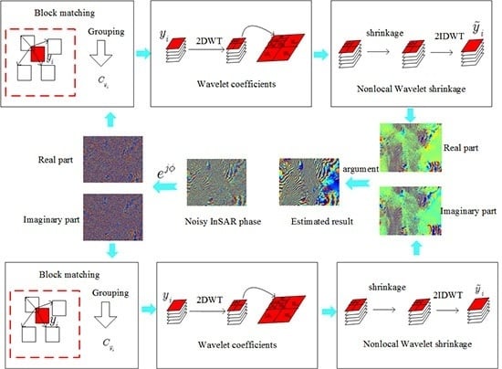
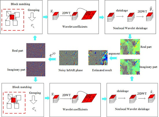
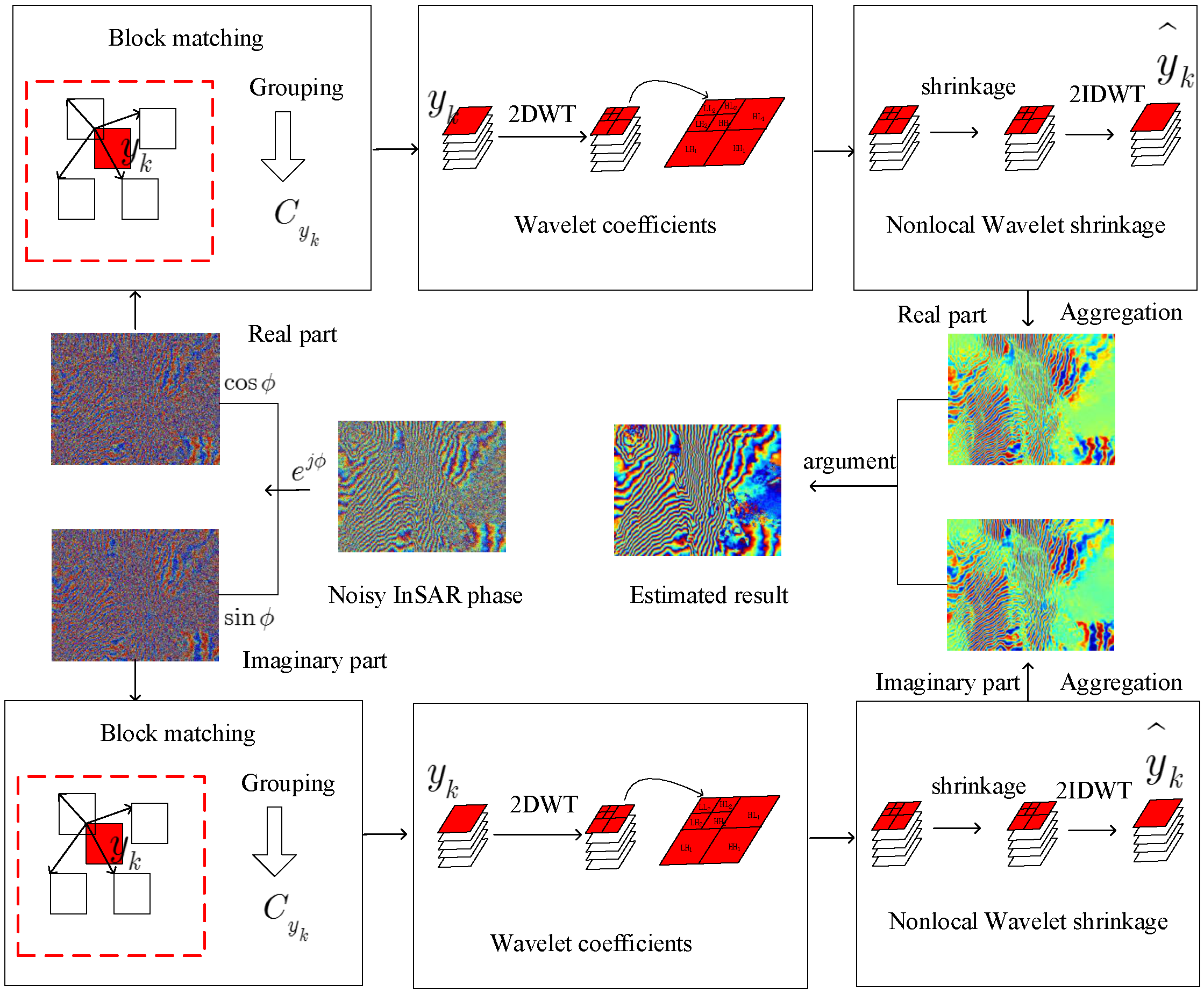
2.2. Modeling of Nonlocal Wavelet Shrinkage Method

For an image x of size $N\times N$ pixels which is corrupted by random noise v, the additive noise observation model of the patch-based method can be expressed as

$$y_i=x_i+v_i$$

(4)

where $y_i$ is a patch of size $M\times M$ pixels that is extracted from y at location i and ordered lexicographically as a column vector $y_i\in R^n$. $x_i$ is the noise-free patch corresponding to $y_i$. $v_i$ is the noise patch. Under the assumption that the solution of upper linear inverse problem has a sparse expansion on an preassigned orthonormal basis, the following shrinkage model is introduced for denoising task using regularization with a sparsity constraint. The recovery problem is solved by an $l_1$-minimization problem

$${\alpha }_i=arg\underset{\begin{array}{c}{\alpha }_i\end{array}}{min}\frac{1}{2}\parallel y_i-T_{2D}^{-1}{\alpha }_i{\parallel }_2^2+\lambda \parallel {\alpha }_i{\parallel }_1$$

(5)

where λ is the regularization multiplier, ${\alpha }_i$ is the coefficient in some transformed basis, and $T_{2D}^{-1}$ is the linear inverse transform.

Wavelet transform (WT) denoising is very promising because the phase information and noise can be more easily separated in the wavelet domain. For an effective restoration, the wavelet shrinkage coefficients, achieved by solving the objective function in Equation (5), are expected to be as close as possible to the true coefficients. Let us define ${\beta }_i$ as the true WT coefficients of $x_i$ (or a good estimation). The estimated ${\alpha }_i$ may deviate from ${\beta }_i$ due to the degradation of the observed $y_i$. In order to get approximate coefficients, we need to minimize ${\gamma }_i={\alpha }_i-{\beta }_i$. Here we call it “wavelet coding noise” and build the regularization model as

$$({\alpha }_i,{\beta }_i)=arg\underset{\begin{array}{c}{\alpha }_i,{\beta }_i\end{array}}{min}\frac{1}{2}\parallel y_i-T_{2D}^{-1}{\alpha }_i{\parallel }_2^2+{\lambda }_1\parallel {\alpha }_i{\parallel }_1+{\lambda }_2\parallel {\alpha }_i-{\beta }_i{\parallel }_p$$

(6)

where ${\alpha }_i$ is the estimated WT coefficients for patch $x_i$, ${\beta }_i$ is a good estimation of the real WT coefficients for patch $x_i$. ${\lambda }_1$ and ${\lambda }_2$ are the Lagrangian multipliers that are used to balance two regularization terms. p is the regularization norm for “wavelet coding noise” term.

Recently, many statistical approaches emerged as new tools for wavelet-based denoising, such as the Bivariate Shrinkage method [24]. The estimation of clean coefficients is expressed as a Bayesian estimation problem, such as the MAP estimator. In Equation (6), ${\beta }_i$ is treated as a peer hidden variable that can be utilized to promote more accurate shrinkage method. Under the Bayesian formula, the posterior estimator is formulated as

$$({\alpha }_i,{\beta }_i)=arg\underset{\begin{array}{c}{\alpha }_i,{\beta }_i\end{array}}{max}log(P({\alpha }_i,{\gamma }_i|y_i))=arg\underset{\begin{array}{c}{\alpha }_i,{\beta }_i\end{array}}{max}\{log(P(y_i|{\alpha }_i,{\gamma }_i))+log(P({\alpha }_i,{\gamma }_i))\}$$

(7)

According to probability theory, there is a relationship: $P({\alpha }_i,{\gamma }_i)=P({\gamma }_i|{\alpha }_i)P({\alpha }_i)$. The distribution of probability $P({\alpha }_i,{\gamma }_i|y_i)$ is characterized by Gaussian distribution as

$$P({\alpha }_i,{\gamma }_i|y_i)=\frac{1}{\sqrt{2}{\sigma }_{{\omega }_i}}exp(-\frac{1}{2}{\sigma }_{{\omega }_i}^2\parallel y_i-T_{2D}^{-1}{\alpha }_i{\parallel }_2^2)$$

(8)

where ${\sigma }_{{\omega }_i}$ is the noise standard deviation of $y_i$. It should be pointed out that the Laplacian distribution for the clean wavelet coefficients is very meaningful [25]. Thus, ${\alpha }_i$ is modeled as the Laplacian distribution

$$P({\alpha }_i)=\frac{1}{\sqrt{2}{\sigma }_{{\alpha }_i}}exp(\frac{\sqrt{2}\parallel {\alpha }_i{\parallel }_1}{{\sigma }_{{\alpha }_i}})$$

(9)

${\gamma }_i$ is also modeled as a Laplacian distribution

$$P({\gamma }_i)=\frac{1}{\sqrt{2}{\sigma }_{{\gamma }_i}}exp(\frac{\sqrt{2}\parallel {\alpha }_i-{\beta }_i{\parallel }_1}{{\sigma }_{{\gamma }_i}})$$

(10)

where ${\sigma }_{{\alpha }_i}$ is the standard deviation of the clean coefficients of patch $x_i$. ${\sigma }_{{\gamma }_i}$ is the standard deviation of ${\gamma }_i$.

Substituting Equations (8)–(10) into Equation (7), we obtain

$$({\alpha }_i,{\beta }_i)=arg\underset{\begin{array}{c}{\alpha }_i,{\beta }_i\end{array}}{min}\frac{1}{2}\parallel y_i-T_{2D}^{-1}{\alpha }_i{\parallel }_2^2+\frac{\sqrt{2{\sigma }_{{\omega }_i}^2}}{{\sigma }_{{\alpha }_i}}\parallel {\alpha }_i{\parallel }_1+\frac{\sqrt{2{\sigma }_{{\omega }_i}^2}}{{\sigma }_{{\gamma }_i}}\parallel {\alpha }_i-{\beta }_i{\parallel }_1$$

(11)

From the point view of the Bayesian estimation, we can see that Equation (11) is equivalent to Equation (6). The regularization term of $\parallel {\alpha }_i-{\beta }_i{\parallel }_p$ should use the $l_1$ norm ($p=1$).

Also, we can set ${\lambda }_1=\frac{\sqrt{2{\sigma }_{{\omega }_i}^2}}{{\sigma }_{{\alpha }_i}}$ and ${\lambda }_2=\frac{\sqrt{2{\sigma }_{{\omega }_i}^2}}{{\sigma }_{{\gamma }_i}}$. It is a double-$l_1$ convex optimization problem [26]. It can be solved by alternatively updating ${\alpha }_i$ via iterative algorithm [27] following the iterative shrinkage solution (see Appendix A)

$${\alpha }_i^{(j+1)}=\left\{\begin{array}{c}{S}_{{\tau }_1,{\tau }_2,{\beta }_i}({\upsilon }_i^{(j)}),{\beta }_i\ge 0\hfill \\ -S_{{\tau }_1,{\tau }_2,{\beta }_i}(-{\upsilon }_i^{(j)}),{\beta }_i<0\hfill \end{array}\right.$$

(12)

where ${\upsilon }^{(j)}=\frac{1}{c}{T_{2D}^{-1}}^T(x-T_{2D}^{-1}{\alpha }^{(j)})+{\alpha }^{(j)}$, ${\tau }_1=\frac{{\lambda }_1}{c}$, and ${\tau }_2=\frac{{\lambda }_2}{c}$. c is an auxiliary parameter guaranteeing the convexity of surrogate function. j denotes the number of iterations. Subscript i denotes the i-th entry in a vector. The generalized shrinkage operator $S_{{\tau }_1,{\tau }_2,{\beta }_i}(t)$ is defined by [27]

$$S_{{\tau }_1,{\tau }_2,{\beta }_i}(t)=\left\{\begin{array}{c}t+{\tau }_1+{\tau }_2,t<-{\tau }_1-{\tau }_2\hfill \\ 0,-{\tau }_1-{\tau }_2<t<{\tau }_1-{\tau }_2\hfill \\ t-{\tau }_1+{\tau }_2,-{\tau }_1-{\tau }_2<t<{\tau }_1-{\tau }_2+b\hfill \\ b,-{\tau }_1-{\tau }_2+b<t<{\tau }_1+{\tau }_2+b\hfill \\ t-{\tau }_1-{\tau }_2,t>{\tau }_1-{\tau }_2+b\hfill \end{array}\right.$$

(13)

where b is the scalar component of ${\beta }_i$.

2.3. Nonlocal Estimation of ${\beta }_i$

It’s impossible to directly obtain the true WT coefficients of clean interferogram because it cannot be directly measured. Since the $2\pi$-periodic nature of the interferometric phase provides abundant self-similar structure, many harmonious patches that we call “groups” can be extracted by clustering or grouping. Figure 1 illustrates the nonlocal self-similar patches in acquired InSAR phase images. The patches in solid line are similar to the reference patch in dash line. In the adaptive estimation strategy, the nonlocal means is introduced in [19]. All similar pixels in its neighborhood can be used to estimate the value. As the patches in one group exhibit perfect similarity, each patch should get some approximately same significant transform coefficients. Inspired by this, the WT coefficients in one similar group can be utilized to get a good estimation of ${\beta }_i$ in the wavelet domain. It can be computed as the weighted average of those WT coefficients associated with the nonlocal similar patches.

For a patch $y_i$, similar patches can be extracted and expressed as a group $C_i=\left\{y_l\right|y_l\mathit{is\; similar\; to}{y}_i,l=1,2,...,K_{num}\}$. $K_{num}$ is the number of patches for one group. The k-th coefficient of ${\beta }_i$ can be estimated by

$${\widehat{\beta }}_{i,k}=\sum _{\begin{array}{c}l\in C_i\end{array}}{\omega }_{i,l}{\alpha }_{l,k}$$

(14)

where ${\alpha }_{l,k}$ is the $k-$th coefficient of ${\alpha }_l$. ${\omega }_{i,l}$ is the weight, which determines the contribution factor for patch $y_l$ in denoising the reference patch $y_i$.

$${\omega }_{i,l}=\frac{1}{\omega }{e}^{-\frac{d(y_i,y_l)}{h}}$$

(15)

where ω is the normalization factor with

$$\omega =\sum _{\begin{array}{c}l\in C_i\end{array}}{\omega }_{i,l},$$

(16)

h is a constant proportional to the noise deviation and can take values as $h=12{\sigma }_{\omega }$. Since the nonlocal structural self-similarity are utilized to estimate ${\beta }_i$, the updating of ${\alpha }_i$ is conducted following the iterative shrinkage solution in Equation (A7). Therefore, the local sparsity in wavelet domain and the nonlocal structural self-similarity are combined in phase denoising.

3. Algorithm Implementation

3.1. Parameter Selection

Interferometric phase noise is spatially variant. Therefore, the filtering parameter should be estimated locally and adjusted to obtain a better filtering performance. For a patch $y_i$, a local estimator of ${\sigma }_{{\omega }_i}$ [28] is

$${\sigma }_{{\omega }_i}=1.4826Med(\mid ▽y_i-Med(▽y_i)\mid );$$

(17)

where ‘$Med(M)$’ is to obtain the median value of M. $▽y_i$ is the gradient of $y_i$.

In wavelet domain, the relation of noisy coefficients, clean coefficients, and noise coefficients are formulated as follows

$$W{y}_i=W{x}_i+W{v}_i$$

(18)

where $W{y}_i$ are noisy coefficients of patch $y_i$, $W{x}_i$ and $W{v}_i$ are clean coefficients, and noise coefficients, respectively. The signal and noise are assumed independent [12]. Hence, ${\sigma }_{{\alpha }_{W{y}_i}}^2={\sigma }_{{\alpha }_i}^2+{\sigma }_{{\alpha }_{W{v}_i}}^2$. The standard deviation of noisy coefficients ${\sigma }_{{\alpha }_{W{v}_i}}$ is estimated as the method in [12], which is

$${\sigma }_{{\alpha }_{W{y}_i}}=\sqrt{\sum _{m=1}^M\sum _{n=1}^M(W{y}_i{(m,n)}^2-{\overline{W{y}_i}}^2)}$$

(19)

where $\overline{W{y}_i}$ is the mean value of the noisy wavelet coefficients $W{y}_i$. According to the method of [13], the standard deviation of noise WT coefficients is

$${\sigma }_{{\alpha }_{W{v}_i}}=Med(\mid W{y}_{HH1}\mid -Med(W{y}_{HH1}))/0.6745$$

(20)

where $W{y}_{HH1}$ represents the wavelet coefficients in the first level HH wavelet subband. After obtaining the values of ${\sigma }_{{\alpha }_{W{y}_i}}$ and ${\sigma }_{{\alpha }_{W{v}_i}}$, ${\sigma }_{{\alpha }_i}$ is calculated using the relation

$${\sigma }_{{\alpha }_i}=\sqrt{Max({\sigma }_{{\alpha }_{W{y}_i}}^2-{\sigma }_{{\alpha }_{W{v}_i}}^2,eps)}$$

(21)

where ‘$eps$’ is a small positive value. ‘$Max$’ operation is to ensure ${\sigma }_{{\alpha }_i}$ is not positive. ${\lambda }_1$ can be calculated as ${\lambda }_1=\frac{\sqrt{2{\sigma }_{{\omega }_i}^2}}{{\sigma }_{{\alpha }_i}}$, ${\lambda }_2$ can be setting as ${\lambda }_2=1-{\lambda }_1$.

3.2. Processing Steps

Figure 2 is the flowchart of the proposed InSAR phase filtering algorithm. As discussed in Section 2.1, the nonlocal structural similarity of the real and imaginary parts of the phase is derived separately. Thus, the filtering is applied to the real and imaginary parts separately. The patches are processed by successively extracting similar patches as one similar group. Grouping is accomplished using the block matching [21]. Each patch is filtered by the nonlocal wavelet shrinkage Equation (A7). Due to the overlapping operation, the patch-based representation is highly redundant. Therefore, the recovery of x from $x_i$ becomes an over-determined problem. A final estimation is made by aggregating all of the obtained local estimates using a weighted average. The filtered blocks are then returned to their original positions. The step-by-step description is given next.

Step 1. Grouping by the block matching:

For each $M\times M$ size reference patch $y_i$ in the original noisy image (real part or imaginary part), find the blocks $y_l$ that are similar to the current processed one, and then cluster them together as a group $C_i$, i.e., $C_i=\left\{y_l\right|d(y_i,y_l)<d^{hard}\}$. The original noisy image is searched for in a reference block-centered $W\times W$ neighborhood. This is achieved by the pairwise-testing the similarity between the reference fragment and the candidate fragments located at the nonlocal spatial locations. Here $l^2$-distance is selected in the identification of the similar blocks

$$d(y_i,y_l)=\frac{\parallel y_i-y_l{\parallel }_2^2}{M^2}$$

(22)

As the noise will influence the precision of similarity adjudgment, it is reasonable to use a higher threshold $d^{hard}$ to select enough similar patches, i.e., $d^{hard}=\frac{{\pi }^2}{4}$. In order to restrict the number of similar patches, the K-nearest neighbor strategy is also implemented. $K_{num}$ patches with the smallest dissimilarity are chosen to be the similar patches of the reference patch. For each similar group, weights $w_{i,l}$ can be calculated and saved, and are used in Step 3 to calculate ${\beta }_i$.

Step 2. Discrete wavelet transform (DWT):

For every block in each group $C_i$, the data are transformed into the wavelet domain.

Step 3. Calculation of nonlocal mean value of wavelet coefficients:

Since nonlocal weights are obtained in Step 1, the nonlocal mean value of the wavelet coefficients in each group is calculated using Equation (15). ${\lambda }_1$ and ${\lambda }_1$ can be calculated by the method of Section 3.1.

Step 4. Nonlocal wavelet shrinkage by double-header $l_1$ optimization:

For each group, the wavelet coefficients are shrunk using Equation (A7).

Step 5. Inverse wavelet transform and aggregation:

The filtered data are inversely transformed into the spatial domain. The aggregation or an averaging procedure that takes advantage of the redundancy is carried out. Similar to the BM3D and the nonlocal filtering method based on the higher order singular value decomposition (HoSVD) [23], a processed pixel can be in different groups by the overlapped patches. Thus, the result after the filtering has to be returned to its original position and to be weighted by an averaging of the block-wise estimates.

Step 6. Estimation updating:

The estimation of recovered phase image is updated by

$$Y^{j+1}=Y^j+\delta (Y-Y^j)$$

(23)

where δ is a pre-determined positive constant controlling the amount of the noise fed back to the iteration. Then, the procedures from Step 1 to Step 6 is iteratively performed until the changes of estimations between two consecutive loops are less than a threshold. The average change of estimations is expressed as $d_p=\frac{1}{N^2}{\sum }_{m=1}^N{\sum }_{n=1}^N[Y^{j+1}(m,n)-Y^j(m,n)]$. This threshold can be chosen according to your filtering precision, such as 1/50 or even smaller.

Step 7. Phase calculation:

Once the real and imaginary parts of the InSAR phase are estimated, the filtered phase image is obtained from

$${\varphi }_e=arg(real+1i·imaginary)$$

(24)

where $arg()$ represents the argument of a complex quantity.

4. Results

It should be noted that the details preservation is very vital for evaluating the quality of the filtering methods. The structural similarity (SSIM) index offers a direct way to compare the structural similarity of the reference and the filtered image when the reference image is available. The SSIM for two windowed reference patch i and filtered patch j can be expressed as [29],

$$SSIM(i,j)=\frac{(2{\mu }_i{\mu }_j+C_1)(2{\sigma }_{ij}+C_2)}{({\mu }_i^2+{\mu }_j^2+C_1)({\sigma }_i^2+{\sigma }_j^2+C_2)}$$

(25)

where ${\mu }_i$ and ${\mu }_j$ are the means of reference patch and the filtered patch, respectively. ${\sigma }_{ij}$ is the covariance of the reference patch and the filtered patch. $C_1$ and $C_2$ are constants to avoid instability when ${\mu }_i^2+{\mu }_j^2$ or ${\sigma }_i^2+{\sigma }_j^2$ is very close to zero. SSIM is distributed in the interval of $[-1,1]$. The structural preservation quality is worst when SSIM is $-1$ and best when SSIM is $-1$. A mean SSIM (MSSIM) index [29] is utilized to evaluate the overall quality as $MSSIM=\frac{1}{K}{\sum }_{i=1}^{M}SSIM(i,j)$.

The metrics for edge preservation such as root-mean-square errors (RMSEs) [23] and SSIM are not available when the reference/clean phase image is unknown. For acquired InSAR data, the reference/clean image is not available. The no-reference metric Q [30] is shown good visual performance in balancing between denoising and detail preservation, so it can be used as a quantitative measure of true phase image content.

In addition, different wavelet bases (Haar wavelet, Daubechies wavelets, bi-orthogonal spline wavelet) are implemented in the developed algorithm. The searching window is limited within the size of $58\times 58$ pixels. The block size is $16\times 16$ pixels. A fixed value $K_{num}=20$ is determined in grouping step. The proposed algorithms are implemented in MATLAB R2013b on a 64 bit 3.10 GHz Intel^® core^TM i5-2400 computer with 16 Gb random access memory (RAM).

4.1. Simulated InSAR Data

The data are simulated using an available DEM. The interferogram data without noise are $512\times 512$ pixels with different fringe densities (Figure 3). For a single-look interferometric phase, the variance of phase noise can be calculated as ${\sigma }_n^2=\frac{{\pi }^2}{3}-\pi arcsin(|\rho |)+{arcsin}^2(|\rho |)-\frac{L{i}_2{(|\rho |}^2)}{2}$. Here $L{i}_2(·)$ is Euler’s dilograrithm. ρ is the coherence. According to four coherence values of 0.3, 0.5, 0.7, and 0.9, we then add Gaussian noise with zero mean and variance ${\sigma }_n^2$. The related interferogram datasets are Data-I (Figure 4A1), Data-II (Figure 4B1), Data-III (Figure 4C1) and Data-IV (Figure 4D1). Noise exists and varies spatially (Figure 4A1–D1). Also, the higher the coherence value is, the less the noise in the InSAR phase data (e.g., Figure 4D1 c.f. Figure 4A1). After three iterations with our developed algorithm, we can obtain satisfactory results. There is significant reduction in noise (e.g., Figure 4A2 c.f. Figure 4A1). The edges of the interferogram is well delineated since the nonlocal wavelet shrinkage method can preserve edges well even though the coherence values are low in phase data. In comparison of the noise-free data (Figure 3) with each filtered phase dataset (Figure 4A2–D2), they look similar. To analyze fringe details preservation, SSIM maps are calculated and shown in Figure 4. Figure 4A3–D3 are SSIM maps between clean phase image and noisy images. Figure 4A4–D4 are SSIM maps between clean phase image and filtered phase images. After filtering, the SSIM values are dramatically increased. Meanwhile, the similarity increases as coherence level increases. For example, the SSIM value in Figure 4D4 are higher than that in Figure 4A4.

We then compute differences of Figure 3 and Figure 4A2, Figure 3 and Figure 4B2, Figure 3 and Figure 4C2, and Figure 3 and Figure 4D2, respectively, and show the differences as Figure 4A5–D5. Difference exists, varies spatially and can be large (e.g., Figure 4A5). Difference values along the transect (shown as a white segment in Figure 3) for the four difference images are extracted and shown (Figure 4A6–D6). The difference ranges from about $-2.5$ to 1.5 rad in Figure 4A6, and from about $-0.15$ to 0.15 rad in Figure 4D6. It is clear the algorithm performs better when the coherence value is high.

The number of residues, RMSEs and MSSIM for each dataset before (

Table 1. Number of residues (#), RMSEs and MSSIM of simulated data before filtering.

	Data-I	Data-II	Data-III	Data-IV
#	76,502	57,680	33,340	7974
RMSEs	2.3814	1.7890	1.1673	0.4795
MSSIM	0.0209	0.0503	0.1111	0.2816

) and after (

Table 2. Number of residues (#), RMSEs and MSSIM of simulated data after filtering with different wavelet bases.

	Data-I			Data-II			Data-III			Data-IV
Filtering Methods	#	RMSEs	MSSIM	#	RMSEs	MSSIM	#	RMSEs	MSSIM	#	RMSEs	MSSIM
Haar	23	0.1115	0.6774	0	0.0222	0.8232	0	0.0094	0.8828	0	0.0037	0.9265
Db2	34	0.1273	0.6609	0	0.0249	0.8164	0	0.0102	0.8781	0	0.0040	0.9236
Db4	27	0.1138	0.6774	0	0.0231	0.8222	0	0.0096	0.8821	0	0.0038	0.9254
Db6	30	0.1186	0.6722	0	0.0241	0.8191	0	0.0099	0.8802	0	0.0039	0.9233
Bior1.3	19	0.1074	0.6828	0	0.0219	0.8244	0	0.0093	0.8834	0	0.0037	0.9261
Bior1.5	19	0.1059	0.6854	0	0.0219	0.8246	0	0.0092	0.8828	0	0.0037	0.9255

) filtering are listed. Comparative experiments are conducted to test the effectiveness and robustness of our proposed method. The transformations are $Haar$, the Haar wavelet, $Dbp$, the Daubechies wavelet with p (p = 2, 4, 6) vanishing moments, $Bior1.N_r$, bi-orthogonal spline wavelet with the vanishing moments of the decomposing and the reconstructing wavelet functions being 1 and $N_r$. From Table 2, we can see that the filtering results with different wavelet bases are very close. The number of residues and RMSEs decrease. For example, the number of residues decrease from 76,502 to 19, and the RMSE from 2.3814 to 0.1059 for Data-I. MSSIM represents the total structural preservation quality. Via comparing Table 1 and Table 2, one can see that MSSIM is above 0.65 even when the phase noise is very high (Data-I). Thus, the performance of the algorithm is quantitatively satisfactory.

4.2. Acquired InSAR Data

The algorithm is further applied to three acquired datasets (Figure 5A1–C1). Data-V (Figure 5A1) and Data-VI (Figure 5B1) are from the airborne C-band SAR using repeat-pass interferometry. Fringes in Data-VI are not as clearly visible as those in Data-V. Data-VI is much noisier than Data-V. Coherence values in Data-V are high (Figure 5A2), but low in Data-VI (Figure 5B2). Data-VII is acquired by the SIR-C/X-SAR mission. Data-VII is selected because the variable fringe density (Figure 5C1) and low-coherence values (Figure 5C2) in mountainous areas.

Interferogram data after filtering are shown in Figure 5A3–C3. When the coherence is high (Figure 5A2), the filtering performs well (Figure 5A3). The fringes are clearly delineated. The performance is satisfactory (Figure 5B3) even if the interferogram is very noisy (Figure 5B1) and the coherence is low (Figure 5B2). The fringes are better depicted (c.f. Figure 5B3 vs. Figure 5B1). The filtered result (Figure 5C3) is still acceptable although the fringes may be not very well delineated in low coherence area. For further analysis on noise reduction and structural preservation, number of residues and metric Q before and after filtering are given in

Table 3. Number of residues (#) and metric Q of acquired dateset before filtering.

	Data-V	Data-VI	Data-VII
#	42,863	54,673	51,599
metric Q	0.0964	0.0596	0.0445

and

Table 4. Number of residues (#) and metric Q of acquired dateset after filtering with different wavelet bases.

	Data-V		Data-VI		Data-VII
	#	Metric Q	#	Metric Q	#	Metric Q
Haar	219	7.6778	228	6.5505	313	6.0949
Db2	243	7.4972	222	6.5601	293	6.0813
Db4	307	7.0544	249	6.4012	315	6.0873
Db6	309	7.0296	233	6.4854	317	6.1029
Bior1.3	328	6.8942	266	6.3551	312	6.0660
Bior1.5	267	6.3835	304	6.0703	322	6.0596

. Via using our proposed method, the number of residues decreases significantly. Overall, the method performs satisfactorily for the interferogram data of variable fringe densities and coherence values.

5. Discussion

5.1. Comparison with Several Interferometric Phase Filters

Several interferometric phase filtering methods are compared. They are frequency domain method (Goldstein [7]), wavelet interferometric phase filter (WInPF) [11], nonlocal based methods (BM3D method [21], modified patch-based locally optimal Wiener (PLOW) method [28] and nonlocal filtering method based on HoSVD (NlHoSVD) [23]).

In simulate experiment, pixels are clustered by using LARK-based K-means cluster in PLOW method methods. In BM3D method, 3D transform is implemented by exploiting 2D bior1.5 wavelet transform for the inter-block and 1D ‘Haar’ wavelet for intra-blocks. In NLHoSVD method, similar patches are formed as a “order-3 tensor” and then HOSVD is applied to the order-3 tensor.

Results from the simulated data using the methods are presented in Figure 6. Quantitative assessment is tabulated in

Table 5. Quantitative assessment of filtered results for simulated data using several widely-used filtering methods (# is the number of residues).

	Data-I			Data-II			Data-III			Data-IV
Filtering Methods	#	RMSEs	MSSIM	#	RMSEs	MSSIM	#	RMSEs	MSSIM	#	RMSEs	MSSIM
Goldstein	43,145	1.5159	0.0299	4077	0.4093	0.1243	472	0.1917	0.4354	71	0.1601	0.6853
WInPF	3943	0.7911	0.2127	1081	0.2500	0.4385	143	0.0875	0.6338	23	0.0325	0.7972
PLOW	889	0.3277	0.4441	38	0.0635	0.6919	0	0.0167	0.8317	0	0.0083	0.8759
BM3D	1184	0.2420	0.4215	22	0.0606	0.6639	0	0.0135	0.8518	0	0.0044	0.9160
NlHoSVD	93	0.2089	0.6345	0	0.0374	0.8300	0	0.0152	0.8913	0	0.0052	0.9351

. Four points are summarized in the comparison study (Figure 4 vs. Figure 6, Table 2 vs. Table 5).

(1)

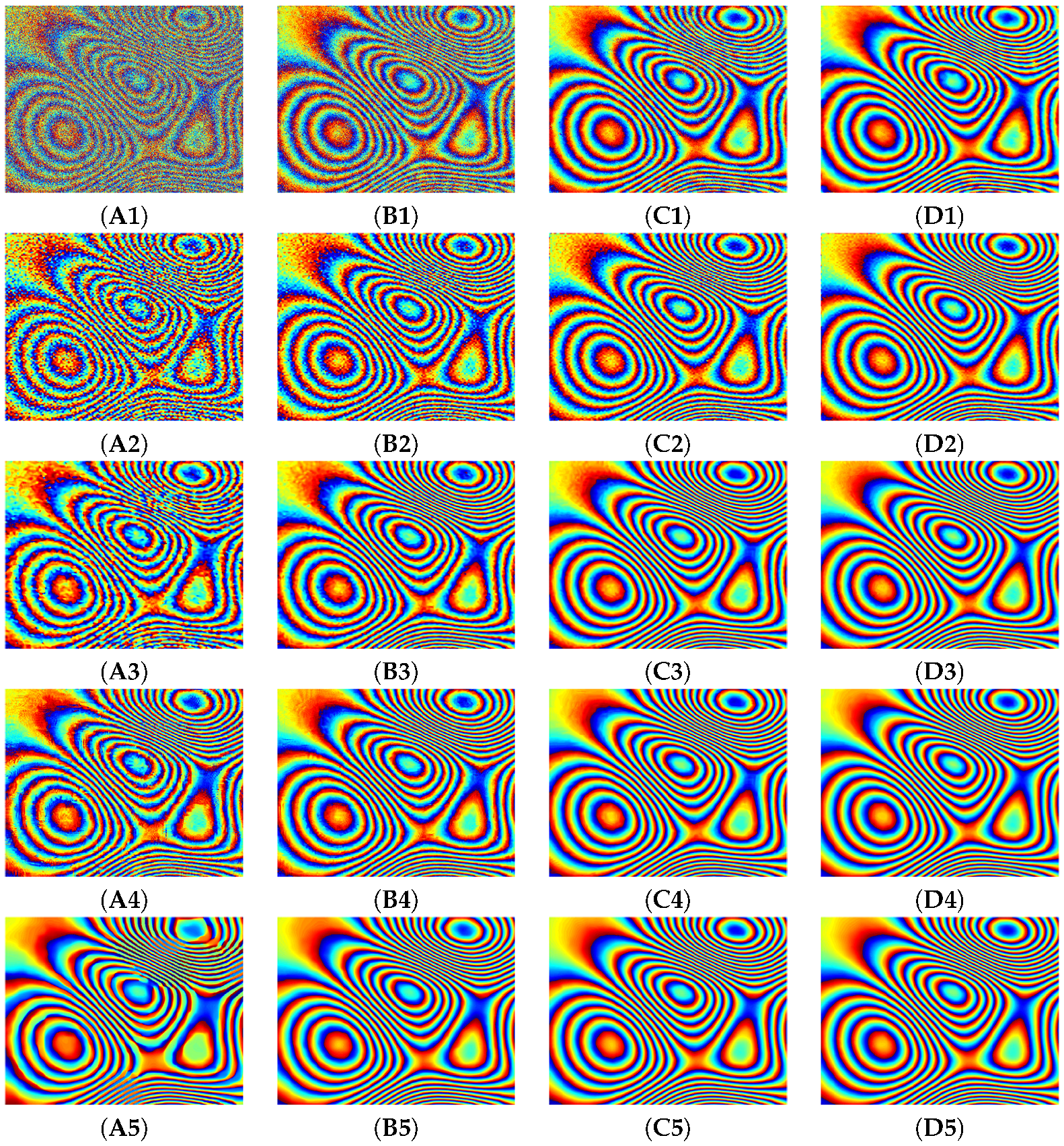
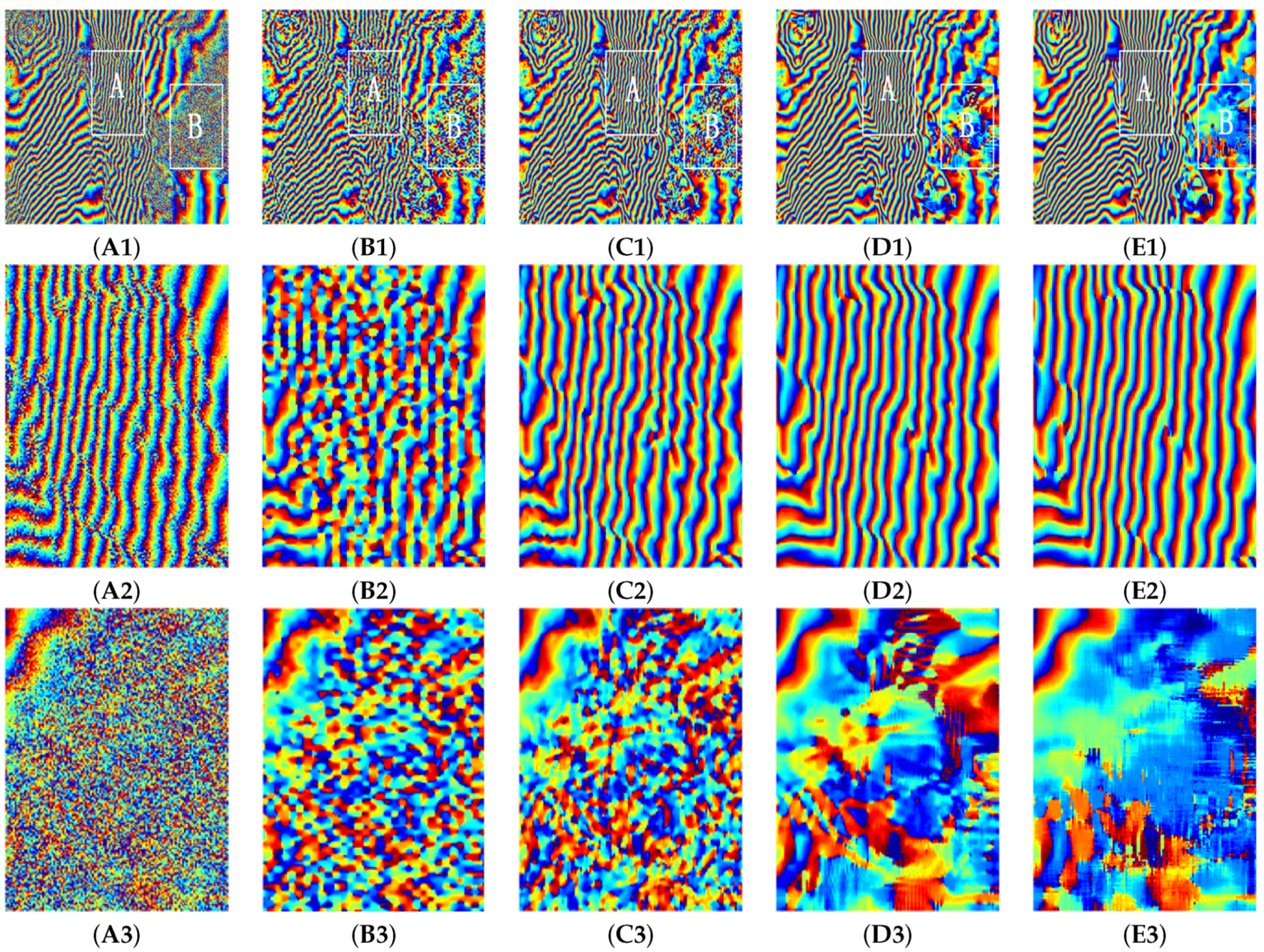
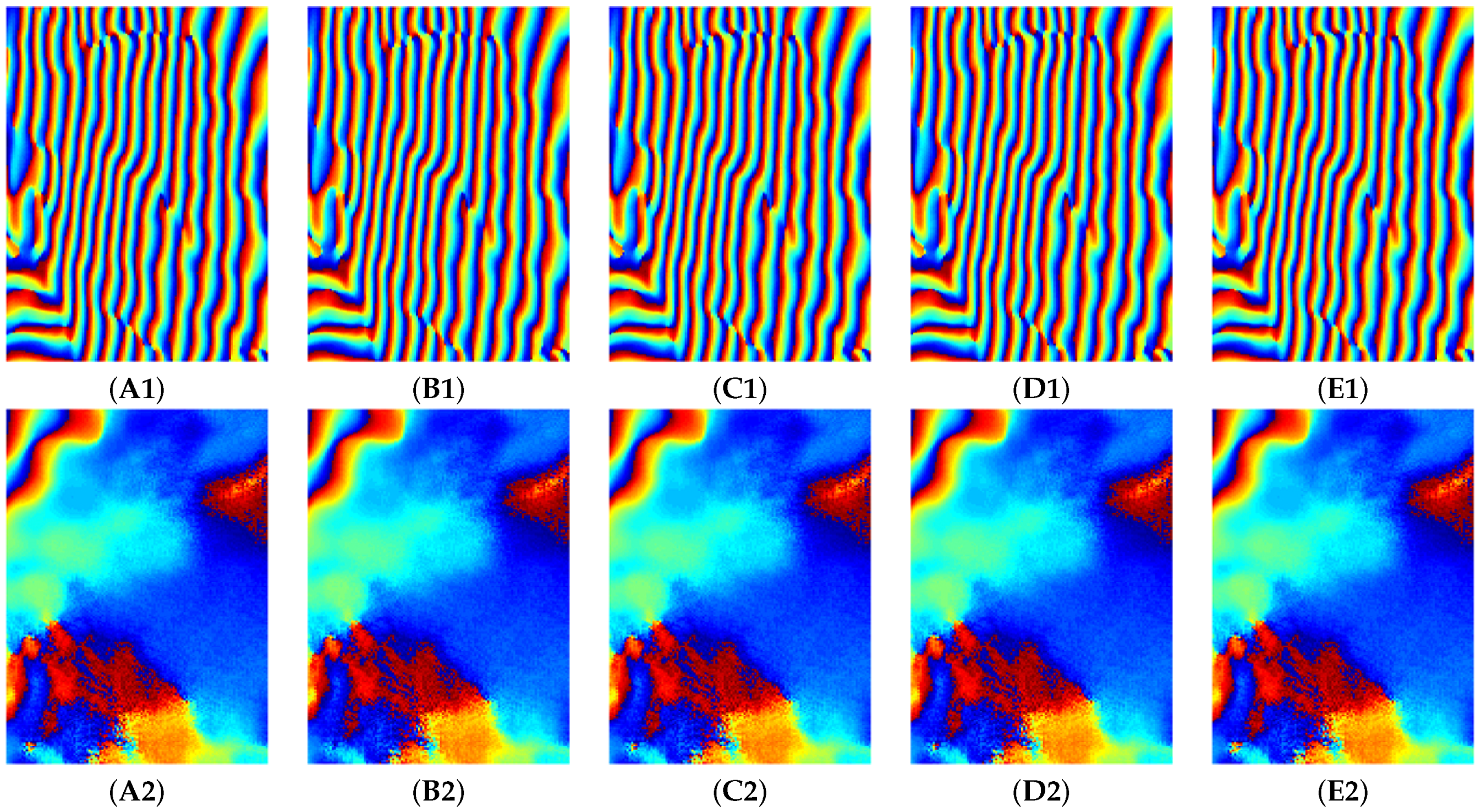
The Goldstein method and the WInPF method show large numbers of errors in almost all the areas of phase image, especially in areas of low coherence value and high fringe density. The number of residues increases with the increase of noise level. The texture in the region of dense fringes is not well preserved.

(2)

The noise suppressing performance of nonlocal based methods is superior than Goldstein and WInPF methods. According to PLOW based on LARK feature method, some phase noise still exists since one cluster may have different noise levels. Some fringes in Figure 6A3 are broken or merged with neighboring fringes.

(3)

The filtering performance of BM3D is comparable to NLHoSVD when the coherence is relatively high. Its details preservation are probably weakened with the presence of strong noise or low signal-to-noise ratio in low-coherence areas. The performance of NlHoSVD is better than that of Goldstein, WInPF, BM3D or PLOW. However, the filter employs the simple hard thresholding method such that the nonlocal similarity might not be fully exploited.

(4)

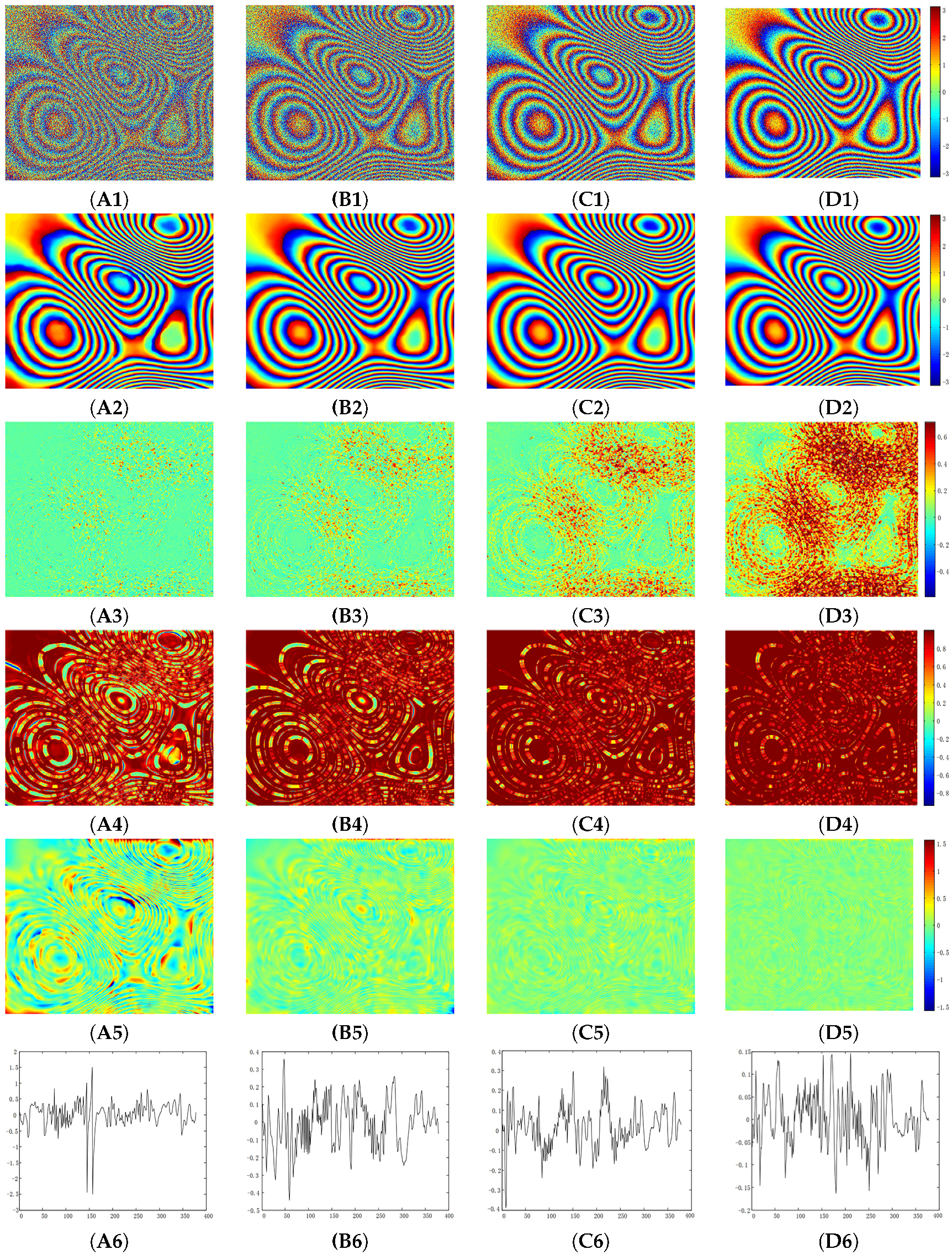
Dataset-by-dataset, the proposed method has the least number of residues and the smallest RMSE (Table 2 c.f. Table 5). In the simulation experiment of Data-II, Data-III and Data-IV, the numbers of residues are all zeros. In addition, the method overcomes the problems of the discontinuity and blurring, and suppresses the phase residues of grainy noise even in areas of low coherence and high fringe.

Similarly, the four methods are used to the acquired data. Pixels are clustered according to their coherence in modified patch-based locally optimal Wiener (PLOW) method [28]. As examples, filtered results for Data-VII are given in Figure 7. From the left to right, the results are from the Goldstein, WInPF, modified PLOW, BM3D and NlHoSVD. Close-up views of area within the white rectangle A and B are shown in the second and third row, respectively. The average coherence value of area A is 0.37 and area B is 0.27.The coherence of area B is very low (See the coherence Figure 5C2). Overall, all methods reduce noise. The Goldstein filter may introduce some artifacts in the areas of severe-phase variation and low coherence, especially in the regions affected by the grainy noise. As compared to results from the Goldstein method, both WInPF methods and nonlocal based methods improve the performance of noise reduction and effectively suppress the residues. The filtered results from WInPF method become worse in the area of low coherence with broken fringes and spike-like fringes (Figure 7B2,B3). However, the modified PLOW, BM3D and NlHoSVD methods significantly suppress noise even in the relatively low-coherence area A. In the very low coherence area B, filtering result of NlHoSVD method is better than the modified PLOW and BM3D methods. The close-up view of the area within the rectangle area A and B from the proposed method is shown in Figure 8. Comparing Figure 7 and Figure 8, we can see that our method in area B is more smooth than other methods. Clearly, the filtered result has the least amount of blurring and discontinuity in phase fringes. The proposed method has the smallest number of residues and the smallest RMSEs (Table 4 c.f.

Table 6. Performance comparison of different methods.

Filtering Methods	#	Metric Q	Computational Time
Interferogram of Data-VII	51,599	0.0445	-
Goldstein	21,043	1.7703	0.2
WInPF	3279	2.0228	0.4
Modified PLOW	2066	4.9825	650.8 s
BM3D	659	5.8600	303.1 s
NlHoSVD	346	5.8994	665.8 s
Our method	322	6.0596	546.0 s

). In the aspect of detail preservation, metric Q is utilized as a quantitative measure of true phase image content. It can be seen that our proposed method can obtain the highest metric Q. From this point of view, our proposed method is superior to the other methods. The processing time for each method is also given in Table 6. The Goldstein method is the fastest one with 0.2 s, and the NlHoSVD is the slowest one with 665.8 s. The processing time of the proposed method is 546.0 s.

5.2. Fast and Efficient Realization

Although the filtering result of our method is convincing, the computational efficiency is intuitively low because it needs pixel-wise window group matching in which the Euclidian distance between similar patches and the weights in the image is computed. For a $N\times N$ phase image with $W\times W$ searching window and $M\times M$ patch size, the complexity of the block matching is $O(\frac{M^2{W}^2{N}^2}{N_{step}^2})$ by setting $N_{step}$ pixel steps between neighboring processed patches. However, the computational complexity can be reduced by restricting the searching size of similar window, steps and patch size. Once the window size and patch size is chosen, further expedients are utilized to improve the computational efficiency in the following:

The Summed Squares Image (SSI) scheme and Fast Fourier Transform (FFT) are proposed [31] to speed up the calculation of similarity among blocks. The Euclidian distance between image blocks is transformed to computation of convolution and summation of squares. In particular, to calculate the distance d between patch $N_1$ and $N_2$, we assume the patch size is $M=2s+1$, then the distance is

$$\begin{array}{cc}\hfill d& =\parallel N_1-N_2{\parallel }^2\hfill \\ & =\sum _{\begin{array}{c}x\end{array}}\sum _{\begin{array}{c}y\end{array}}{(S_1(x,y)-S_2(x,y))}^2\hfill \\ & =\sum _{x=1}^{2s+1}\sum _{y=1}^{2s+1}(S_1^2(x,y))+\sum _{x=1}^{2s+1}\sum _{y=1}^{2s+1}(S_2^2(x,y))-2\sum _{x=1}^{2s+1}\sum _{y=1}^{2s+1}{S}_1(x,y)S_2(x,y)\hfill \\ & =\sum _{x=1}^{2s+1}\sum _{y=1}^{2s+1}(S_1^2(x,y))+\sum _{x=1}^{2s+1}\sum _{y=1}^{2s+1}(S_2^2(x,y))-2\sum _{x=1}^{2s+1}\sum _{y=1}^{2s+1}{S}_1(x,y)S_3(2s+1-x+1,2s+1-y+1)\hfill \\ & =\sum _{x=1}^{2s+1}\sum _{y=1}^{2s+1}(S_1^2(x,y))+\sum _{x=1}^{2s+1}\sum _{y=1}^{2s+1}(S_2^2(x,y))-2S_1(x,y)*S_3(m,n)\hfill \end{array}$$

(26)

where $S_1$ and $S_2$ are the corresponding pixels in image patch $N_1$ and $N_2$, respectively. $S_3$ is the mirrored image of $S_2$ with $m=2S+1$ and $n=2S+1$ (Figure 9).

The first and second terms in Equation (26) need to calculate the sum of squares [31] for any block. The sum of squares for each pixel in any rectangles of the image can be got using SSI. For example in Figure 10, the sum of squares in rectangle A can be expressed as

$$K(x_1,y_1)=\sum _{x\le x_1}\sum _{y\le y_1}S{(x,y)}^2$$

(27)

To calculate the sum of squares in rectangle D, only 3 addition operations are required,

$$\begin{array}{cc}\hfill K_D& =S_{A\bigcup B\bigcup C\bigcup D}+S_A-S_{A\bigcup C}-S_{A\bigcup B}\hfill \\ & =K(x_2,y_2)+K(x_1,y_1)-K(x_1,y_2)-K(x_2,y_1)\hfill \end{array}$$

(28)

With the SSI, the sum of squares for each pixel in any rectangle can be derived only by additional operations. Since each pixel in the original image is only processed once, the computational complexity for computing the SSI is $O(N^2)$. The third term is calculated by convolution with multiplifications under the FFT. In order to accelerate the algorithm, convolution and summation of squares are utilized in calculating $l^2$-distance.

In our experiments, convolution and summation of squares are utilized in calculating Euclidian distance. The processing time of accelerated method is 176.6 s. The computational time is reduced and accelerated 3.1 times with respect to the original method.

6. Conclusions

In order to preserve fringe details in InSAR denoising processing, especially when dealing with a low-coherence and high-noise area, we develop an InSAR phase filtering algorithm in wavelet domain that utilizes the local sparsity of wavelet coefficients and nonlocal similarity of grouped blocks. In the algorithm, the double-$l_1$ norm restriction is used, which enforces the local and nonlocal sparsity constraints by efficient shrinkage operators. The nonlocal similar blocks of interferogram are clustered by block matching, and then the overlapped blocks are shrunk in 2D wavelet domain by the nonlocal wavelet shrinkage function. The filter combines the intra- and inter-blocks correlation. Thus, the finest details shared by the grouped blocks and the essential unique features of each individual block are revealed.

Four sets of simulated phase data and three sets of acquired data are used to assess the performance of the proposed method. The simulated InSAR datasets are with high-dense fringes and different level of noise. Results demonstrate the algorithm’s ability to filter noise and to preserve fringe texture even in areas of low coherence and high fringe density. Three acquired datasets with variable fringe densities are analyzed. The outcomes are satisfactory.

For comparison, four widely-used interferometric phase filtering methods are applied to the datasets. Qualitative assessments show that the proposed method outperforms the state-of-the-art with lower root-mean-square error, and less noisy fringes.

References

1. Eichel, P.H.; Ghiglia, D.C.; Jakowatz, C.V., Jr. Spotlight SAR Interferometry for Terrain Elevation Mapping and Interferometric Change Detection; SAND93-2072 UC-700; Sandia National Labs.: Albuquerque, NM, USA; AT and T Technologies, Inc.: Albuquerque, NM, USA, 1996; Volume 12.
2. Lanari, R.; Fornaro, G. Generation of digital elevation models by using SIR-C/X-SAR multifrequency two-pass interferometry: The Etna case study. IEEE Trans. Geosci. Remote Sens. 1996, 34, 1097–1114. [Google Scholar] [CrossRef]
3. Lee, J.S.; Papathanassiou, K.P.; Ainsworth, T.L.; Grunes, M.R.; Reigber, A. A new technique for noise filtering of SAR interferometric phase images. IEEE Trans. Geosci. Remote Sens. 1998, 36, 1456–1465. [Google Scholar]
4. Wu, N.; Fang, D.; Li, J. A locally adaptive filter of interferometric phase images. IEEE Geosci. Remote Sens. Lett. 2006, 3, 73–77. [Google Scholar] [CrossRef]
5. Cai, B.; Liang, D.; Dong, Z. A New Adaptive Multiresolution noise filtering approach for SAR interferometric phase images. IEEE Geosci. Remote Sens. Lett. 2008, 5, 266–270. [Google Scholar]
6. Yu, Q.; Xia, Y.; Fu, S.; Sun, X. An adaptive contoured window filter for interferometric synthetic aperture radar. IEEE Geosci. Remote Sens. Lett. 2006, 3, 73–77. [Google Scholar] [CrossRef]
7. Goldstein, R.M.; Werner, C.L. Radar interferogram filtering for geophysical application. Geophys. Res. Lett. 1998, 25, 4035–4038. [Google Scholar] [CrossRef]
8. Baran, I.; Stewart, M.P.; Kampes, B.M.; Perski, Z.; Lilly, P. A modification to the Goldstein radar interferogram filter. IEEE Trans. Geosci. Remote Sens. 2003, 41, 2114–2118. [Google Scholar] [CrossRef]
9. Li, Z.; Bao, Z.; Li, H.; Liao, G. Image autocoregistration and InSAR interferogram estimation using joint subspace projection. IEEE Trans. Geosci. Remote Sens. 2006, 44, 288–297. [Google Scholar]
10. Lopez-Martinez, C.; Fabregas, X. Modeling and reduction of SAR interferometric phase noise in the wavelet domain. IEEE Trans. Geosci. Remote Sens. 2002, 40, 2553–2566. [Google Scholar] [CrossRef]
11. Martinez, C.L.; Canovas, X.F.; Chandra, M. SAR interferometric phase noise reduction using wavelet transform. Electron. Lett. 2003, 37, 649–651. [Google Scholar] [CrossRef]
12. Zha, X.; Fu, R.; Dai, Z.; Liu, B. Noise reduction in interferograms using the wavelet packet transform and wiener filtering. IEEE Geosci. Remote Sens. Lett. 2008, 5, 404–408. [Google Scholar]
13. Donoho, D.L.; Johnstone, I.M. Ideal spatial adaptation by wavelet shrinkage. Biometrika 1994, 81, 425–455. [Google Scholar] [CrossRef]
14. Chen, G.Y.; Bui, T.D.; Krzyzak, A. Image denoising with neighbor dependency and customized wavelet and threshold. Pattern Recognit. 2005, 38, 115–124. [Google Scholar] [CrossRef]
15. Bian, Y.; Mercer, B. Interferometric SAR phase filtering in the wavelet domain using simultaneous detection and estimation. IEEE Trans. Geosci. Remote Sens. 2010, 49, 1396–1416. [Google Scholar] [CrossRef]
16. Xu, G.; Xing, M.; Xia, X.; Zhang, L.; Liu, Y.; Bao, Z. Sparse regularization of interferometric phase and amplitude for InSAR image formation based on Bayesian representation. IEEE Trans. Geosci. Remote Sens. 2015, 53, 2123–2136. [Google Scholar] [CrossRef]
17. Bhateja, V.; Tripathi, A.; Gupta, A.; Lay-Ekuakille, A. Speckle suppression in SAR images employing modified anisotropic diffusion filtering in wavelet domain for environment monitoring. Measurement 2015, 74, 246–254. [Google Scholar] [CrossRef]
18. Xu, B.; Cui, Y.; Zuo, B.; Yang, J.; Song, J. Polarimetric SAR image filtering based on patch ordering and simultaneous sparse coding. IEEE Trans. Geosci. Remote Sens. 2016, 54, 4079–4093. [Google Scholar] [CrossRef]
19. Buadeset, A.; Coll, B.; Morel, J. A review of image denoising algorithms, with a new one. Multiscale Model. Simul. 2005, 4, 490–530. [Google Scholar] [CrossRef]
20. Buades, A.; Coll, B.; Morel, J.M. Nonlocal image and movie denoising. Int. J. Comput. Vis. 2008, 76, 123–139. [Google Scholar] [CrossRef]
21. Dabov, K.; Foi, A.; Katkovnik, V.; Egiazarian, K. Image denoising by sparse 3-D transform-domain collaborative filtering. IEEE Trans. Image Process. 2007, 16, 2080–2095. [Google Scholar] [CrossRef] [PubMed]
22. Deledalle, C.A.; Denis, L.; Tupin, F. NL-InSAR: Nonlocal interferogram estimation. IEEE Trans. Geosci. Remote Sens. 2011, 49, 1441–1452. [Google Scholar] [CrossRef]
23. Lin, X.; Li, F.; Meng, D.; Hu, D. Nonlocal SAR interferometric phase filtering through higher order singular value decomposition. IEEE Geosci. Remote Sens. Lett. 2015, 12, 806–810. [Google Scholar] [CrossRef]
24. Sendur, L.; Selesnick, I.W. Bivariate shrinkage functions for wavelet-based denoising exploiting interscale dependency. IEEE Geosci. Signal Process. 2002, 50, 2744–2756. [Google Scholar] [CrossRef]
25. Martinez, L.; Canovas, F.; Javier, F. SAR interferometric phase statistics in wavelet domain. Electron. Lett. 2002, 38, 1207–1208. [Google Scholar]
26. Zibulevsky, M.; Elad, M. L1-L2 optimization in signal and image processing. Signal Process. Mag. 2010, 27, 76–88. [Google Scholar] [CrossRef]
27. Dong, W.; Li, X.; Zhang, L.; Shi, G. Sparsity-based image denoising via dictionary learning and structural clustering. In Proceedings of the IEEE Conference on Computer Vision and Pattern Recognition (CVPR), Colorado Springs, CO, USA, 20–25 June 2011; pp. 457–464.
28. Wang, Y.; Huang, H.; Dong, Z.; Wu, M. Modified patch-based locally optimal wiener method of interferometric SAR phase filtering. J. Photogramm. Remote Sens. 2016, 114, 10–23. [Google Scholar] [CrossRef]
29. Wang, Z.; Bovik, A.C.; Sheikh, H.R.; Simoncelli, E.P. Image quality assessment: From error visibility to structural similarity. IEEE Trans. Image Process. 2004, 13, 600–612. [Google Scholar] [CrossRef] [PubMed]
30. Zhu, X.; Milanfar, P. Automatic parameter selection for denoising algorithms using no-reference measure of image content. IEEE Trans. Image Process. 2010, 19, 3116–3132. [Google Scholar] [PubMed]
31. Wang, J.; Guo, Y.; Ying, Y.; Liu, Y.; Peng, Q. Fast non-local algorithm for image denoising. In Proceedings of the IEEE International Conference on Image Processing, Atlanta, GA, USA, 8–11 October 2006; pp. 1429–1432.
Figure 1. Nonlocal structure of InSAR phase. (Dashed rectangles denote reference patches, and solid rectangles are similar patches.)
Remotesensing 08 00830 g001
Figure 2. Flowchart of the nonlocal wavelet shrinkage method.
Remotesensing 08 00830 g002
Figure 3. Simulated phase data without noise. The white segment is a transect.
Remotesensing 08 00830 g003
Figure 4. Analysis of simulated data. (A1D1) are simulated Data-I, Data-II, Data-III, and Data-IV consisting of noise, respectively; (A2D2) are the filtered results of (A1D1) by using the proposed method (Here we only show the filtered results with Bior1.5 wavelet); (A3D3) are SSIM maps of noisy phase image A1 and Figure 3, B1 and Figure 3, C1 and Figure 3, D1 and Figure 3; (A4D4) are SSIM maps of the filtered phase image A2 and Figure 3, B2 and Figure 3, C2 and Figure 3, D2 and Figure 3; (A5D5) are difference images of Figure 3 and A2, Figure 3 and B2, Figure 3 and C2, and Figure 3 and D2; (A6D6) are values of (A2D2) along the transect shown as a white segment in Figure 3.
Remotesensing 08 00830 g004
Figure 5. Analysis of acquired interferometric data. Data-V (A1), Data-VI (B1) and Data-VII (C1) are acquired interferogram data. (A2C2) are the coherence values of (A1C1), respectively. (A3C3) are filtered results using the proposed method.
Remotesensing 08 00830 g005
Figure 6. Filtered results of simulated Data-I, Data-II, Data-III and Data-IV. (A1D1) are results using the Goldstein method; (A2D2) are results by the WInPF; (A3D3) are results using PLOW method; (A4D4) are results using BM3D method; (A5D5) are results by the nonlocal filtering method based on HoSVD.
Remotesensing 08 00830 g006
Figure 7. Results for acquired Data-VII after several phase filtering methods. (A1) Goldstein; (B1) WInPF; (C1) Modified FLOW; (D1) BM3D; (E1) NlHoSVD. (A2E2) Close-up views within the rectangle areas A are shown in the second row, respectively. (A3E3) Enlarged area B are shown in the third row, respectively.
Remotesensing 08 00830 g007
Figure 8. Results for acquired Data-VII after our proposed filtering methods with different wavelet bases. (A1) Haar; (B1) Db2; (C1) Db4; (D1) Bior1.3; (E1) Bior1.5. (A1E1) Close-up views within the rectangle areas A are shown in the first row, respectively. (A2E2) Enlarged area B are shown in the second row, respectively.
Remotesensing 08 00830 g008
Figure 9. A mirrored image.
Remotesensing 08 00830 g009
Figure 10. Using SSI to compute the summed squared pixels in rectangle D.
Remotesensing 08 00830 g010