Using Google Earth Surface Metrics to Predict Plant Species Richness in a Complex Landscape

Abstract

Google Earth provides a freely available, global mosaic of high-resolution imagery from different sensors that has become popular in environmental and ecological studies. However, such imagery lacks the near-infrared band often used in studying vegetation, thus its potential for estimating vegetation properties remains unclear. In this study, we assess the potential of Google Earth imagery to describe and predict vegetation attributes. Further, we compare it to the potential of SPOT imagery, which has additional spectral information. We measured basal area, vegetation height, crown cover, density of individuals, and species richness in 60 plots in the oak forests of a complex volcanic landscape in central Mexico. We modelled each vegetation attribute as a function of surface metrics derived from Google Earth and SPOT images, and selected the best-supported linear models from each source. Total species richness was the best-described and predicted variable: the best Google Earth-based model explained nearly as much variation in species richness as its SPOT counterpart (R² = 0.44 and 0.51, respectively). However, Google Earth metrics emerged as poor predictors of all remaining vegetation attributes, whilst SPOT metrics showed potential for predicting vegetation height. We conclude that Google Earth imagery can be used to estimate species richness in complex landscapes. As it is freely available, Google Earth can broaden the use of remote sensing by researchers and managers in low-income tropical countries where most biodiversity hotspots are found.

1. Introduction

Remote sensing is a useful tool in environmental and ecological research. This technology allows ecologists to gather information about the natural world more rapidly and cost effectively than traditional field methods, and aid in the analyses and integration of processes across spatial and temporal scales [1]. Remote sensing is useful when studying vegetation to assess ecosystem functioning and health [2], regulate human use of vegetation [3,4], and prioritise areas for conservation and restoration [5,6].

Although Landsat imagery is still the most frequently used source in remote sensing studies [7], some vegetation patterns cannot be captured at its resolution (30 m pixel) [8]. Other sensors such as SPOT (Satellite Pour l’Observation de la Terre), Quickbird, GeoEye-1 and RapidEye produce higher resolution images, but they can be prohibitively expensive for many researchers and managers, particularly in low-income countries. Although financial considerations are important when choosing an image source, the capabilities of different sources need rigorous assessment.

Since its launch in 2005, Google Earth © (GE) has become an application with an enormous impact on research and environmental management, even amongst non-experts in remote sensing. GE provides a collage of free images, many of which have extremely high resolution (up to 15 cm) [9]. GE has mostly been used for visual interpretation of natural- and human-related phenomena, but digital image analysis has seldom been applied to GE images ([10], but see [11]) This is partly due to the lack of the near-infrared (NIR) band in GE images (i.e., they only have the red, green, and blue bands: RGB), without which one cannot calculate widely used vegetation indices such as the Normalized Difference Vegetation Index (NDVI) [12].

Previously, efforts concentrated on predicting vegetation attributes using the raw spectral information in satellite images [13]. More recently, the spatial arrangement of spectral information (i.e., image texture) has also been used [14]. The basic tenet of this approach is that such spatial structure holds a strong correspondence with the heterogeneity of the vegetation [15]. Studies based on image texture have reported high predictability of some vegetation attributes, such as community basal area and tree density (e.g., [16,17]).

Here we assess the potential of spectral and textural information extracted from GE imagery to predict oak forest attributes in a complex volcanic landscape, and compare it to the potential of SPOT imagery. Despite its limited spectral information, we expected the data of high-resolution GE imagery to be a good predictor of vegetation attributes in heterogeneous environments. Considering the substantial reduction in costs and the global availability of GE images, it was important to assess its real predictive potential objectively.

2. Materials and Methods

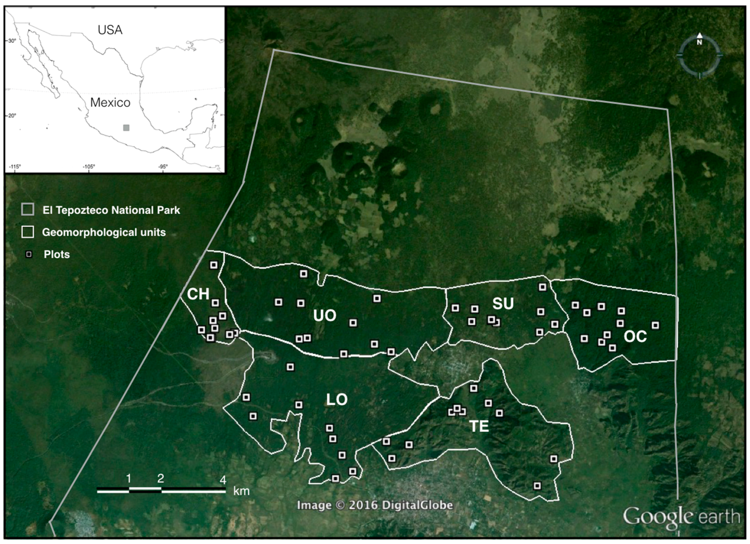
2.1. Study Site

We conducted the study in El Tepozteco National Park, located on the Chichinautzin volcanic range, ca. 50 km south of Mexico City, Mexico (19°01.10′N, 99°05.80′W; Figure 1). It encompasses a complex territory including the Tepozteco Mountains, which are the result of eroded lahars, as well as a mosaic of lava fields with ages ranging from 1835 to >20,000 years old [18,19]. We studied oak forests in six geomorphological units: Tepozteco Mountains (TM), and four lava fields, namely Chichinautzin (CH), Suchiooc (SU), Otates, which is divided into lower (LO) and upper (UO) subunits, and Oclayuca (OC). Overall mean annual temperature is 15.6 °C, and mean total annual precipitation is 2100 mm, with a rainy season between May and October [20]. Climatic conditions vary along the park’s elevational gradient, which ranges from 1350 to 3350 m a.s.l. Oak forests extend from 1800 to 2800 m a.s.l., and shift gradually into conifer forests above, and tropical dry forests below. Additionally, patches of xerophytic vegetation in rocky outcrops and recent lava fields are found amid the oak forests.

2.2. Field Data

We randomly located ten 10 × 10 m plots in each geomorphological unit (Figure 1) and sampled them in October and November 2010 and 2011. We recorded all plant species present in each plot, and for plants with a diameter at breast height (DBH) ≥2.5 cm (hereafter referred to as ‘canopy’), we measured DBH, height and two orthogonal crown diameters (to estimate crown cover as the area of an ellipse). We used these variables to calculate density of individuals, basal area, total crown cover, and vegetation height (mean height of the three tallest trees) in each plot. Also, we calculated species richness and Shannon’s Index [21] for the whole community and for the canopy in each plot.

2.3. Image Processing

We calculated spectral and textural metrics for GE and SPOT 5 images, which were then used to model vegetation attributes. The GE image used in this study was a pansharpened Quickbird image, constructed by mosaicing and georeferencing screenshots captured with a fixed eye altitude of 3 km in Google Earth, while the SPOT image was subjected to geometric correction. We preferred the term GE image instead of its commercial name (Quickbird) to highlight the use of a free image server, and also because we did not have access to the raw Quickbird information. The main differences between these two image sources were: (1) the available bands (RGB in GE; RG and NIR in SPOT), (2) their spatial resolution (GE = 0.75 m; SPOT = 2.5 m), and (3) their acquisition date (January 2005 for GE and March 2010 for SPOT). Although the GE image differed by five years from our field measurements, we decided to use it because it was the only high-resolution image covering the entire study area.

We used only the red band and a vegetation index for each image to calculate the Visible Vegetation Index (VVI) for GE, and the NDVI for SPOT, as follows:

$$\mathrm{VVI}={\left[\left(1-\left|\frac{\mathrm{R}-{\mathrm{R}}_0}{{\mathrm{R}+\mathrm{C}+\mathrm{R}}_0}\right|\right)\left(1-\left|\frac{\mathrm{G}-{\mathrm{G}}_0}{{\mathrm{G}+\mathrm{C}+\mathrm{G}}_0}\right|\right)\left(1-\left|\frac{\mathrm{B}-{\mathrm{B}}_0}{{\mathrm{B}+\mathrm{C}+\mathrm{B}}_0}\right|\right)\right]}^{1/\mathrm{w}}$$

(1)

$$\mathrm{NDVI}=\frac{\mathrm{NIR}-\mathrm{R}}{\mathrm{NIR}+\mathrm{R}}$$

(2)

where NIR, R, G, and B are the near-infrared, the red, the green, and the blue band, respectively, R₀ = 40, G₀ = 60, B₀ = 10, C = 10, and w = 1 [22,23]. Equation 1 is a modification of the original formula following the recommendations of its proponents. These indices were calculated manually in ENVI 5 (Exelis Visual Information Solutions, Boulder, CO, USA).

We calculated 13 surface metrics for each band or vegetation index. Eight were co-occurrence or texture metrics calculated following the grey level co-occurrence method (GLCM; Supplementary Material 1) [24], using an offset of one pixel and a transformation of pixel values to 64 grey levels to minimise computation time. To obtain a rotation-invariant texture measure, all the co-occurrence metrics were calculated in four directions (0°, 45°, 90°, 135°) and then averaged. The remaining five occurrence metrics, also known as spectral metrics, were calculated using raw pixel values (see Supplementary Material 1). We calculated all metrics using the moving window approach [24]. To ensure a good match between window size and sampling plot size, we used a square window of 15 pixels for GE and 5 pixels for SPOT.

2.4. Statistical Analysis

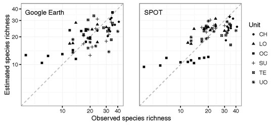
We constructed linear and quadratic models of surface metrics as predictors of vegetation attributes. Higher-order models were not explored because of limited degrees of freedom (n = 60). Thus, we fitted eight types of models:

y = β₀ + β₁x₁,

(3)

y = β₀ + β₁x₁ + β₂x₂,

(4)

y = β₀ + β₁x₁ + β₂x₂ + β₃x₁x₂,

(5)

y = β₀ + β₁x₁ + β₂x₂ + β₃x₃,

(6)

y = β₀ + β₁x₁ + β₂x₁²,

(7)

y = β₀ + β₁x₁ + β₂x₁² + β₃x₂,

(8)

y = β₀ + β₁x₁ + β₂x₁² + β₃x₂ + β₄x₂²,

(9)

y = β₀ + β₁x₁ + β₂x₁² + β₃x₂ + β₄x₁x₂,

(10)

where y is a log-transformed vegetation variable, and x₁, x₂ and x₃ are surface metrics. The normal distribution of the error was verified in all models. All possible combinations of metrics were evaluated.

We calculated the coefficient of determination (R²) as a goodness-of-fit measure for each model. R² has the advantage of having a fixed range (0 to 1, with 1 being a perfect fit), making it easy to interpret. However, R² is not useful for model comparison, as it does not penalise for model complexity. Therefore, our model selection process was based on the Akaike Information Criterion; due to our small sample sizes we used the corrected version (AICc). Two models were considered to be equally supported when ΔAICc < 2 [25].

Given the large number of fitted models and the small sample size of our database, we expected some large R²-values to result purely by chance. To explore this possibility, we randomly sorted the data of each variable, fitted the models, and calculated their associated R². Iteration of this procedure 1000 times allowed us to estimate the distribution of the R²-values under a random scenario, and thus calculate P-values associated with the observed R² values.

We used a leave-two-out cross-validation to evaluate the ability of the different combination of surface metrics to predict vegetation attributes in the models. In this procedure, we split the dataset into a calibration subset (with 58 data points) and a validation subset (two data points), fitted the model to the former, and predicted the vegetation attribute for the latter. Following Gallardo-Cruz et al. [17], we used the leave-d-out cross-validation R²:

R²_CV = 1 − nc⁻¹d⁻¹ Σ_c Σ_d (y_obs − y_pred)²/Σ_n(y_obs − y_avg)²,

(11)

where n is the number of plots, c is the number of possible splits of the data set, y_obs are the observed vegetation-attribute data points, y_pred are the values predicted by the model using the d surface data points, and y_avg is the average over the n vegetation-attribute data points. R²_CV ranges from −∞ to 1, with 1 being a perfect fit, and negative values representing over-fitted models that make worse predictions than chance.

3. Results

Total species richness was the vegetation attribute best described and predicted by the image surface data. It was the only attribute for which both GE and SPOT models had higher R² values than expected by chance (

Table 1. P-values of the R²’s associated with the best model (selected through AICc) for each vegetation variable, image, and model type (following equation numbers in text). Bold typeface, P < 0.05; italics, P < 0.1. BA, basal area; COV, vegetation cover; DEN, density of individuals; HEm, mean vegetation height; HEv, variance in vegetation height; S_can, canopy species richness (i.e., individuals with DBH ≥2.5 cm); S_tot, total species richness; H_can, Shannon diversity of the canopy; H_tot, Shannon diversity of the whole community.

Model Type	BA	COV	DEN	HEm	HEv	Scan	Stot	Hcan	Htot
Google Earth
3	0.580	0.343	0.039	0.587	0.628	0.939	0.519	0.508	0.135
7	0.888	0.743	0.088	0.865	0.958	0.664	0.002	0.611	0.407
7	0.481	0.431	0.170	0.250	0.285	0.715	0.018	0.799	0.093
5	0.557	0.725	0.065	1.000	0.711	0.811	0.002	0.391	0.109
9	0.807	0.809	0.067	0.752	0.793	0.156	0.004	0.717	0.232
8	0.695	0.729	0.186	0.624	0.659	0.916	0.007	0.604	0.197
10	0.778	0.837	0.136	0.955	0.703	0.532	0.004	0.352	0.154
6	0.374	0.306	0.195	0.304	0.388	0.813	0.019	0.694	0.196
SPOT
3	0.486	0.108	0.585	0.002	0.034	0.943	0.001	0.844	0.001
7	0.711	0.162	0.092	0.002	0.189	0.795	0.002	0.988	0.002
4	0.521	0.106	0.567	0.002	0.180	0.784	0.001	0.776	0.004
5	0.853	0.294	0.334	0.004	0.530	0.679	0.001	0.982	0.001
9	0.298	0.378	0.593	0.009	0.239	0.925	0.011	0.952	0.039
8	0.661	0.218	0.332	0.003	0.530	0.915	0.001	0.918	0.001
10	0.793	0.520	0.424	0.010	0.410	0.772	0.002	0.959	0.001
6	0.518	0.119	0.424	0.004	0.238	0.764	0.002	0.743	0.002

). The best models explained about half of the variation in community species richness for both GE and SPOT images (R² = 0.44 and 0.51, respectively;

Table 2. Best models constructed for each vegetation attribute. Only those metrics for which at least one model had a P-value < 0.05 associated to its random R² distribution are shown. Of those, models with a ΔAICc < 2 are shown. In Model type, y is the log-transformed vegetation variable and x₁ and x₂ are the surface metrics described in their respective columns. The + and − signs indicate positive and negative β coefficients, respectively. See Supplementary Material 1 for the mathematical formulation of surface metrics.

Vegetation Attribute	Image	x1	x2	Model Type	ΔAICc	R2	R2CV
Total richness	SPOT	red.cc.mean	red.st.entro	y = β0 + β1x1 − β2x12 − β3x2 + β4x22	0	0.51	0.40
		red.st.mean	red.st.entro	y = β0 + β1x1 − β2x12 − β3x2 + β4x22	0.289	0.50	0.40
		red.st.entro	red.cc.mean	y = β0 − β1x1 + β2x12 + β3x2	1.585	0.47	0.39
	GE	red.cc.asm	vvi.cc.mean	y = β0 + β1x1 − β2x2 − β3x1x2	0	0.44	0.34
		red.cc.asm	vvi.st.mean	y = β0 + β1x1 − β2x2 − β3x1x2	0.365	0.44	0.33
Height mean	SPOT	ndvi.st.entro	red.cc.mean	y = β0 − β1x1 + β2x12 − β3x2 − β4x22	0	0.42	0.31
		red.st.dr	ndvi.st.mean	y = β0 + β1x1 + β2x2	0.493	0.37	0.31
		red.st.dr	ndvi.cc.mean	y = β0 + β1x1 + β2x2	0.632	0.37	0.31
		red.cc.mean	red.cc.hom	y = β0 − β1x1 − β2x12 − β3x2 + β4x22	0.661	0.41	0.25
		red.cc.mean	ndvi.st.entro	y = β0 − β1x1 − β2x2 + β3x1x2	0.704	0.39	0.28
		ndvi.st.entro	ndvi.st.mean	y = β0 − β1x1 + β2x12 + β3x2 − β4x22	0.914	0.41	0.32
		ndvi.st.entro	ndvi.cc.mean	y = β0 − β1x1 + β2x12 + β3x2 − β4x22	1.142	0.41	0.32
		ndvi.st.mean	red.st.dr	y = β0 + β1x1 − β2x12 + β3x2	1.147	0.39	0.31
		red.cc.mean	red.cc.diss	y = β0 − β1x1 − β2x12 − β3x2 + β4x22	1.307	0.41	0.26
		ndvi.cc.hom	red.cc.mean	y = β0 − β1x1 + β2x12 − β3x2 − β4x22	1.356	0.41	0.26
		ndvi.cc.mean	red.st.dr	y = β0 + β1x1 − β2x12 + β3x2	1.398	0.38	0.31
		ndvi.st.entro	red.st.mean	y = β0 − β1x1 + β2x12 + β3x2 + β4x22	1.483	0.41	0.29
		red.cc.mean	ndvi.cc.hom	y = β0 + β1x1 + β2x2 − β3x1x2	1.517	0.38	0.26
		red.st.mean	red.cc.hom	y = β0 + β1x1 − β2x12 − β3x2 + β4x22	1.522	0.40	0.24
		ndvi.st.mean	red.st.var	y = β0 + β1x1 − β2x12 + β3x2	1.917	0.38	0.31
Shannon diversity	SPOT	red.st.entro	red.cc.mean	y = −β0 + β1x1 − β2x12 − β3x2	0	0.42	0.34
		red.st.entro	red.cc.mean	y = −β0 − β1x1 + β2x12 + β3x2 − β4x22	0.856	0.43	0.34
		red.st.entro	red.st.mean	y = −β0 + β1x1 − β2x12 − β3x2	1.918	0.42	0.34
Density	GE	red.st.skew		y = β0 + β1x1	0	0.18	0.07
Height variance	SPOT	ndvi.st.mean		y = β0 + β1x1	0	0.16	0.10
		ndvi.cc.mean		y = β0 + β1x1	0.183	0.15	0.09
		red.cc.mean		y = β0 − β1x1	1.918	0.13	0.07

). In contrast, canopy species richness and vegetation structure were described poorly, and R² values were lower than expected by chance. Exceptions to this were mean vegetation height, which was successfully described by SPOT-based models, and density, which was adequately described by one GE-based model.

All the best models selected by AICc included either one or two surface metrics as predictors (Table 2). Including a third predictor never resulted in better models. While the best models to predict total species richness based on SPOT images included only red-band surface metrics, models based on GE images used both red and VVI metrics.

The accuracy of model estimates of total species richness varied among geomorphological units (Figure 2). The worst predictions were observed for the Oclayuca plots, where the best GE estimated values were close to the average richness of plots in that unit, but failed to distinguish the variation among them. Species richness in the Chichinautzin lava field tended to be underestimated, while it was overestimated for the Lower Otates unit.

4. Discussion

In our rapidly changing world, it is increasingly important to assess and monitor ecosystem properties accurately across landscapes, particularly biodiversity. Satellite-based modelling is a valuable tool to achieve this, but cost still limits the acquisition of high-resolution images [11]. Our results show that GE imagery can be used to describe and predict species richness in heterogeneous environments. Although the best GE models only explained about one half of the variation of the recorded species richness, this result is valuable given the high floristic heterogeneity of the studied forests [26]. Moreover, the performance of GE-based models in describing richness was similar to that of SPOT-based models, a widely used but costly counterpart. It is worth noting that an apparent saturation in the capability of modelling low species richness (under 10 species) from texture metrics is observed in our models (Figure 2). However, these low richness sites correspond to a single geomorphological unit (OC, Oclayuca); therefore we cannot be certain whether the models have limited predictive power in low richness sites, or if it is simply a local effect associated with a given geomorphological unit.

To our surprise, all models failed to describe canopy richness adequately (Table 1), which may be due to the considerably poorer and more homogeneous canopy richness in these oak forests across the landscape, relative to the high richness of the accompanying (i.e., non-canopy) species. One possible explanation is that, due to the relatively small size of our sampling plots (10 × 10 m) compared to the crown of some of the largest trees, in some cases the heterogeneity of pixels within a plot could be more closely associated with the variability within a single tree crown than with the variability among crowns of different tree species.

The most common textural metrics in the best species richness models were cc.mean and cc.asm, both of which are related to the local spectral heterogeneity of pixels in an image. Previously, cc.mean was identified as one of the most capable surface metrics to detect changes in vegetation attributes [17]. The potential of GE images to predict species richness is supported by the fact that the best SPOT models for species richness did not include NIR or NDVI metrics, which suggests that the NIR band is less useful in image-based estimations of species richness, at least in this forest type.

Admittedly, other aspects regarding image acquisition can affect the calculation of GLCM metrics such as pixel size, topography and illumination. Pixel size will determine the scale at which the GLCM texture will summarise patterns of heterogeneity [27]. In this study, the effect of different pixel sizes on the capabilities of GLCM to model forest attributes was not tested. Testing the effect of scale or pixel resolution on the capabilities of texture metrics remains an important task for future texture studies. The effect of topography and acquisition configuration may not affect our results greatly because most of our plots are located in well-illuminated areas and beyond steep areas [28].

All vegetation structure attributes, except vegetation height, were poorly modelled. Interestingly, for estimations of vegetation height, we obtained the sharpest difference in performance between GE and SPOT: while models based on GE images performed poorly, models for SPOT images performed well. The inability of the models based on GE imagery to predict vegetation height adequately is disappointing given the importance of this attribute for biomass estimation [29]. Other important structural attributes such as basal area and vegetation cover have been correctly estimated from surface metrics in other satellite imagery [11,17]. The underlying mechanistic relationships between vegetation attributes and remotely-sensed surface metrics are still blurry, which partially explains the inconsistent results obtained through different methodological approaches and remote sensors [16,30]. However, Gallardo-Cruz et al. [17] showed that for a vegetation attribute to be correctly modelled, it should be highly heterogeneous. In this study, mean vegetation height and species richness differed significantly among geomorphological units; however, while basal area was equally variable among these units, its variation was not significant [31].

5. Conclusions

In a time when global change and biodiversity loss are major threats to ecosystem structure and function, estimating species richness from remote sensing information is of the utmost importance. Among the enormous variety of available high-resolution images, freely available ones have not been tested as widely as their commercial counterparts. In this study, we showed that the limited spectral resolution and lack of metadata of free GE images, in comparison with a commercial one (SPOT) are of minor consequence for its potential to predict plant species richness in heterogeneous landscapes from surface metrics. In addition, GE images can be more user-friendly than commercial counterparts and, in most cases, require no special skills to view or download. Harnessing the predictive potential of GE imagery emerges as an important tool for detecting and managing biodiversity hotspots, especially in tropical regions where researchers and managers have less access to expensive high-resolution imagery.

References

1. Turner, W.; Spector, S.; Gardiner, N.; Fladeland, M.; Sterling, E.; Steininger, M. Remote sensing for biodiversity science and conservation. Trends Ecol. Evol. 2003, 18, 306–314. [Google Scholar] [CrossRef]
2. Chambers, J.Q.; Asner, G.P.; Morton, D.C.; Anderson, L.O.; Saatchi, S.S.; Espírito-Santo, F.D.B.; Palace, M.; Souza, C. Regional ecosystem structure and function: Ecological insights from remote sensing of tropical forests. Trends Ecol. Evol. 2007, 22, 414–423. [Google Scholar] [CrossRef] [PubMed]
3. Pitt, D.G.; Wagner, R.G.; Hall, R.J.; King, D.J.; Leckie, D.G.; Runesson, U. Use of Remote sensing for forest vegetation management: A problem analysis. For. Chron. 1997, 73, 459–477. [Google Scholar] [CrossRef]
4. Franklin, S.E. Remote Sensing for Sustainable Forest Management; CRC Press: Boca Raton, FL, USA, 2001. [Google Scholar]
5. Harris, G.M.; Jenkins, C.N.; Pimm, S.L. Refining biodiversity conservation priorities. Conserv. Biol. 2005, 19, 1957–1968. [Google Scholar] [CrossRef]
6. Holl, K.D.; Aide, T.M. When and where to actively restore ecosystems? For. Ecol. Manag. 2011, 261, 1558–1563. [Google Scholar] [CrossRef]
7. Wulder, M.A.; Masek, J.G.; Cohen, W.B.; Loveland, T.R.; Woodcock, C.E. Opening the archive: How free data has enabled the science and monitoring promise of Landsat. Remote Sens. Environ. 2012, 122, 2–10. [Google Scholar] [CrossRef]
8. Asner, G.P.; Keller, M.; Pereira, R.; Zweede, J.C. Remote sensing of selective logging in Amazonia: Assessing limitations based on detailed field observations, Landsat ETM+, and textural analysis. Remote Sens. Environ. 2002, 80, 483–496. [Google Scholar] [CrossRef]
9. Hu, Q.; Wu, W.; Xia, T.; Yu, Q.; Yang, P.; Li, Z.; Song, Q. Exploring the use of google earth imagery and object-based methods in land use/cover mapping. Remote Sens. 2013, 5, 6026–6042. [Google Scholar] [CrossRef]
10. Barbosa, J.M.; Broadbent, E.N.; Bitencourt, M.D. Remote sensing of aboveground biomass in tropical secondary forests: A review. Int. J. For. Res. 2014, 2014, 1–14. [Google Scholar] [CrossRef]
11. Ploton, P.; Pélissier, R.; Proisy, C.; Flavenot, T.; Barbier, N.; Rai, S.N.; Couteron, P. Assessing aboveground tropical forest biomass using Google Earth canopy images. Ecol. Appl. 2012, 22, 993–1003. [Google Scholar] [CrossRef] [PubMed]
12. Schowengerdt, R.A. Remote Sensing: Models and Methods for Image Processing; Academic Press: San Diego, CA, USA, 2007. [Google Scholar]
13. Pettorelli, N.; Vik, J.O.; Mysterud, A.; Gaillard, J.-M.; Tucker, C.J.; Stenseth, N.C. Using the satellite-derived NDVI to assess ecological responses to environmental change. Trends Ecol. Evol. 2005, 20, 503–510. [Google Scholar] [CrossRef] [PubMed]
14. Haralick, R.M. Statistical and structural approaches to texture. Proc. IEEE 1979, 67, 786–804. [Google Scholar] [CrossRef]
15. Rocchini, D.; Balkenhol, N.; Carter, G.A.; Foody, G.M.; Gillespie, T.W.; He, K.S.; Kark, S.; Levin, N.; Lucas, K.; Luoto, M.; et al. Remotely sensed spectral heterogeneity as a proxy of species diversity: Recent advances and open challenges. Ecol. Inform. 2010, 5, 318–329. [Google Scholar] [CrossRef]
16. Couteron, P.; Pelissier, R.; Nicolini, E.A.; Paget, D. Predicting tropical forest stand structure parameters from Fourier transform of very high-resolution remotely sensed canopy images. J. Appl. Ecol. 2005, 42, 1121–1128. [Google Scholar] [CrossRef] [Green Version]
17. Gallardo-Cruz, J.A.; Meave, J.A.; González, E.J.; Lebrija-Trejos, E.E.; Romero-Romero, M.A.; Pérez-García, E.A.; Gallardo-Cruz, R.; Hernández-Stefanoni, J.L.; Martorell, C. Predicting tropical dry forest successional attributes from space: Is the key hidden in image texture? PLoS ONE 2012, 7, e30506. [Google Scholar] [CrossRef] [PubMed]
18. Siebe, C.; Arana-Salinas, L.; Abrams, M. Geology and radiocarbon ages of Tláloc, Tlacotenco, Cuauhtzin, Hijo del Cuauhtzin, Teuhtli, and Ocusacayo monogenetic volcanoes in the central part of the Sierra Chichinautzin, México. J. Volcanol. Geotherm. Res. 2005, 141, 225–243. [Google Scholar] [CrossRef]
19. Siebe, C.; Rodríguez-Lara, V.; Schaaf, P.; Abrams, M. Radiocarbon ages of Holocene Pelado, Guespalapa, and Chichinautzin scoria cones, south of Mexico City: Implications for archaeology and future hazards. Bull. Volcanol. 2004, 66, 203–225. [Google Scholar] [CrossRef]
20. INEGI (Instituto Nacional de Estadística y Geografía). Cuaderno Estadístico Municipal de Tepoztlán, Morelos. Available online: http://www.inegi.org.mx/est/contenidos/espanol/sistemas/cem03/estatal/mor/m020/index.html (accessed on 5 January 2010).
21. Magurran, A.E. Measuring Biological Diversity; John Wiley & Sons: Oxford, UK, 2004. [Google Scholar]
22. Huete, A.R.; Liu, H.Q.; Batchily, K.; VanLeeuwen, W. A comparison of vegetation indices over a global set of TM images for EOS-MODIS. Remote Sens. Environ. 1997, 5, 6026–6042. [Google Scholar] [CrossRef]
23. Planetary Habitability Laboratory (PHL). Visible Vegetation Index (VVI). Available online: http://phl.upr.edu/projects/visible-vegetation-index-vvi (accessed on 24 August 2016).
24. Haralick, R.M.; Shanmugam, K.; Dinstein, I.’H. Textural features for image classification. Proc. IEEE 1973, 3, 610–621. [Google Scholar] [CrossRef]
25. Burnham, K.P.; Anderson, D.R. Model Selection and Multimodel Inference; Springer: New York, NY, USA, 2002. [Google Scholar]
26. Block, S.; Meave, J.A. Structure and diversity of oak forests in the El Tepozteco National Park (Morelos, Mexico). Bot. Sci. 2015, 93, 429–460. [Google Scholar] [CrossRef]
27. Barbier, N.; Couteron, P.; Proisy, C.; Malhi, Y.; Gastellu-Etchegorry, J.-P. the variation of apparent crown size and canopy heterogeneity across lowland Amazonian forests. Glob. Ecol. Biogeogr. 2010, 19, 72–84. [Google Scholar] [CrossRef]
28. Barbier, N.; Proisy, C.; Véga, C.; Sabatier, D.; Couteron, P. Bidirectional Texture function of high resolution optical images of tropical forest: An approach using LiDAR hillshade simulations. Remote Sens. Environ. 2011, 115, 167–179. [Google Scholar] [CrossRef]
29. Chave, J.; Réjou-Méchain, M.; Búrquez, A.; Chidumayo, E.; Colgan, M.S.; Delitti, W.B.C.; Duque, A.; Eid, T.; Fearnside, P.M.; Goodman, R.C.; et al. Improved allometric models to estimate the aboveground biomass of tropical trees. Glob. Chang. Biol. 2014, 20, 3177–3190. [Google Scholar] [CrossRef] [PubMed]
30. Lu, D.; Batistella, M. Exploring TM image texture and its relationships with biomass estimation in Rondônia, Brazilian Amazon. Acta Amazon. 2005, 35, 249–257. [Google Scholar] [CrossRef]
31. Block, S. Heterogeneidad florística y estructural de los encinares del Parque Nacional El Tepozteco, México. Bachelor’s Thesis, National Autonomous University of Mexico, Mexico City, Mexico, 2013. [Google Scholar]
Figure 1. Google Earth image of the study site captured on January 2005, showing limits of El Tepozteco National Park (Mexico) and location of oak forest sampling plots in six geomorphological units: Chichinautzin (CH), Suchiooc (SU), Otates, divided into a lower (LO) and upper (UO) subunit, and Oclayuca (OC). Extreme coordinates of this scene are 18.977°–19.099°N, 99.024°–99.201°W. Actual geomorphological units are larger than the polygons shown here, as these only depict the extent of oak forest in these units.
Remotesensing 08 00865 g001
Figure 2. Observed species richness vs. species richness estimated by the best descriptive models based on (a) Google Earth and (b) SPOT image surface data. Unit refers to the geomorphological units in the study site.
Remotesensing 08 00865 g002