
Separability Analysis of Sentinel-2A Multi-Spectral Instrument (MSI) Data for Burned Area Discrimination

 , , , , , and
Abstract
:
1. Introduction
2. Data and Pre-Processing
2.1. Sentinel-2 Images
2.2. Sentinel-2 Image Pre-Processing
2.3. Study Spectral Bands and Indices
3. Method
3.1. Burned and Unburned Pixel Sample Collection
3.2. Statistical Separability Analysis
3.2.1. Parametric Separability Analysis
3.2.2. Non-Parametric Separability Analysis
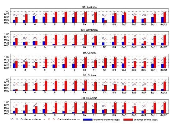
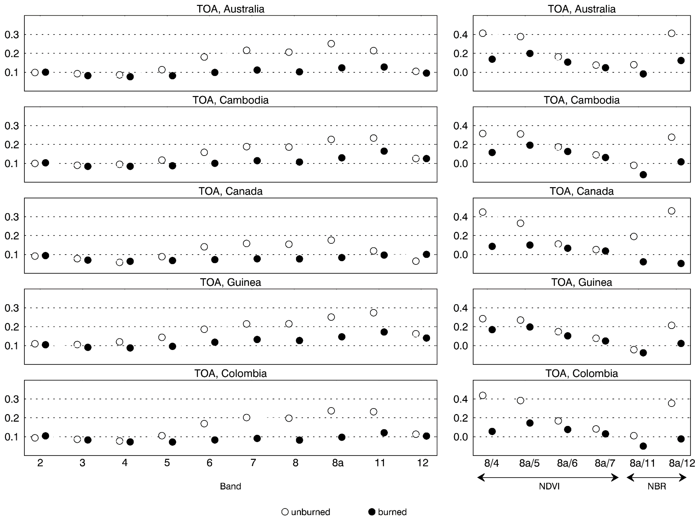
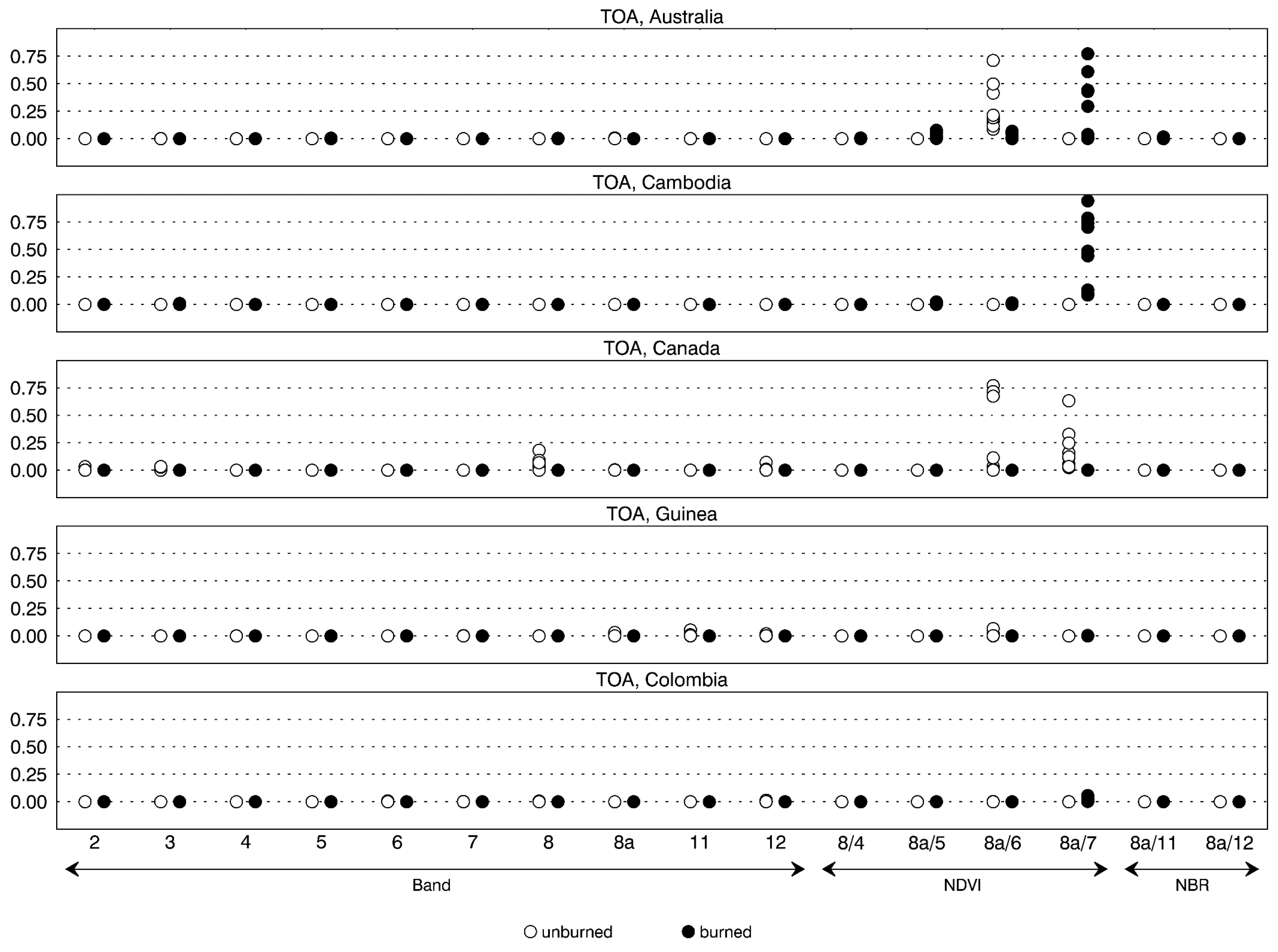
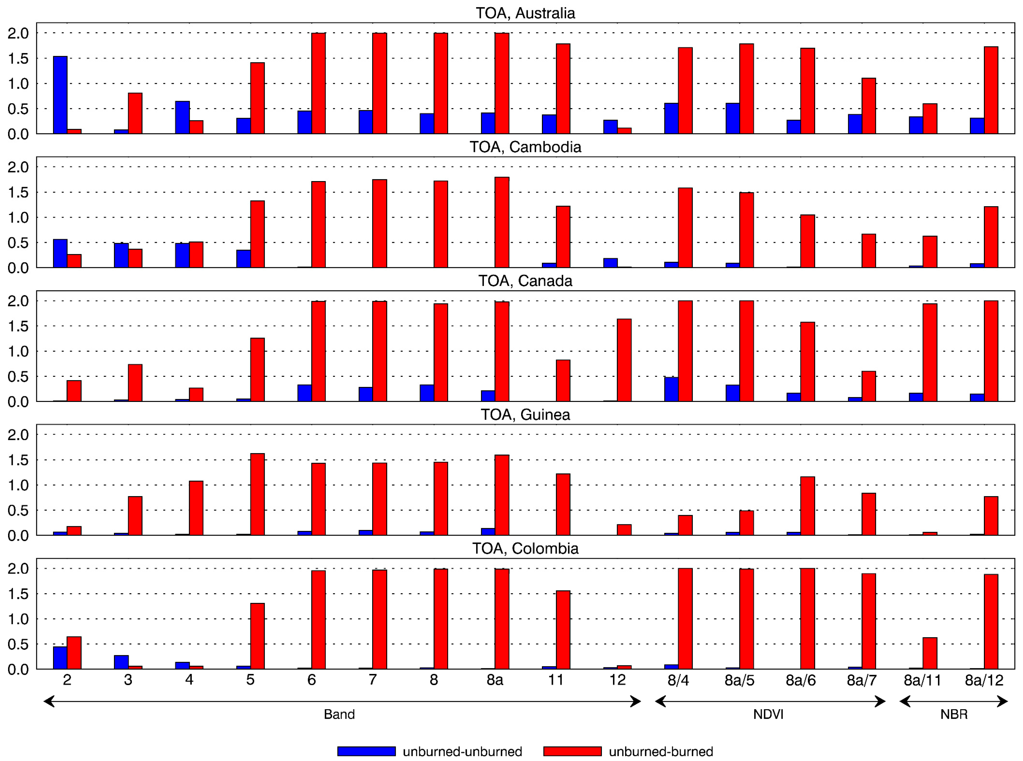
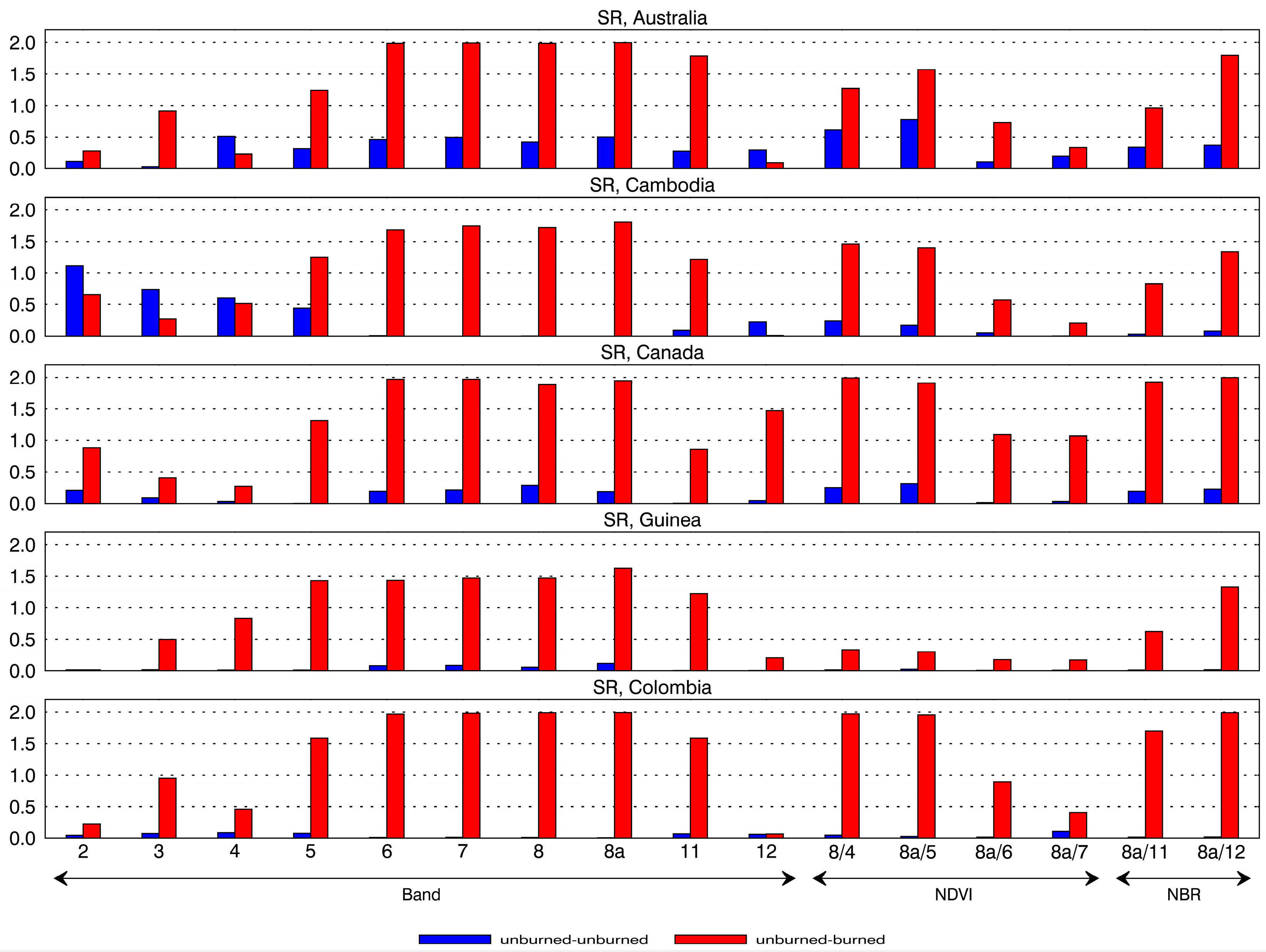
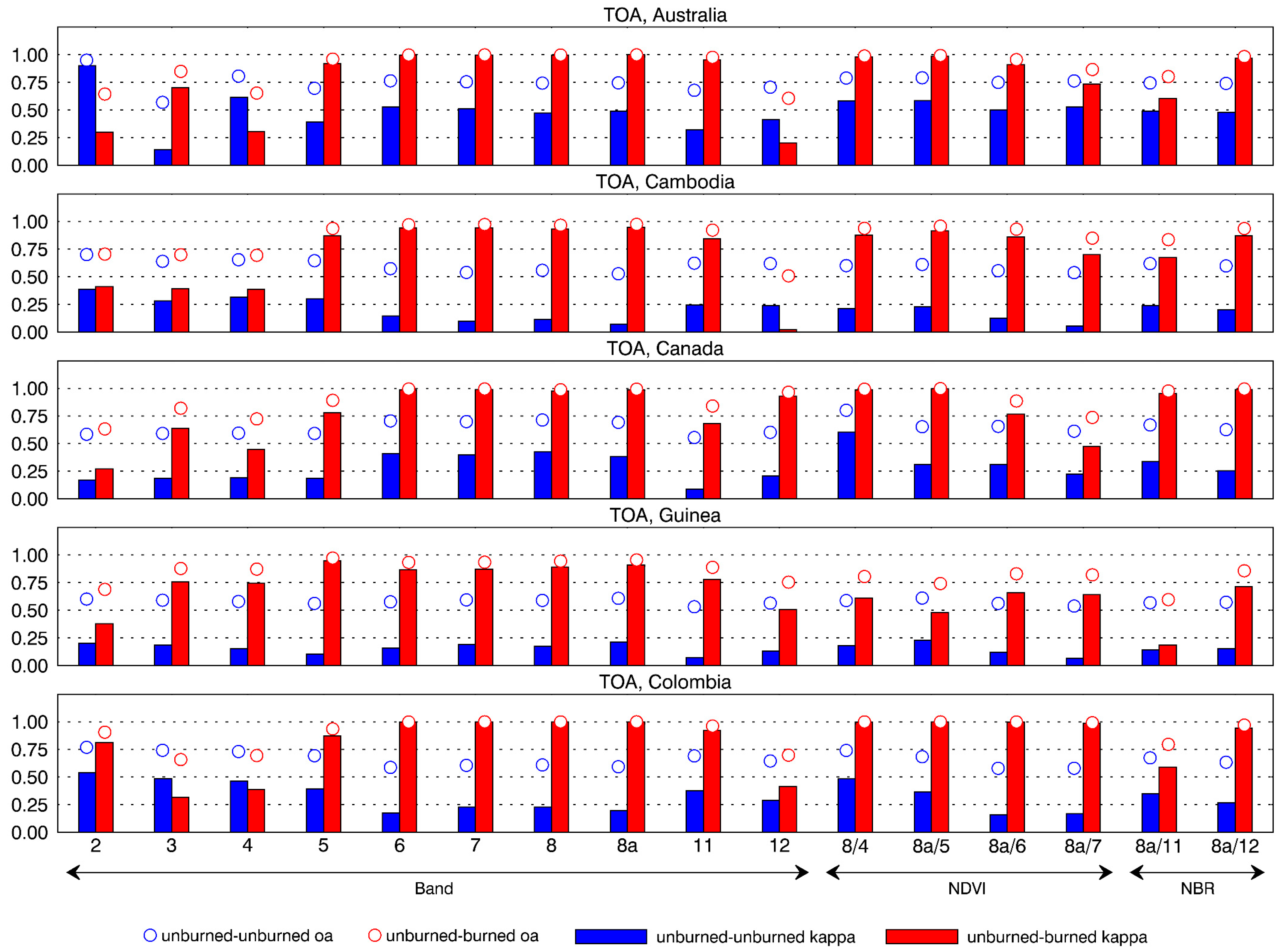
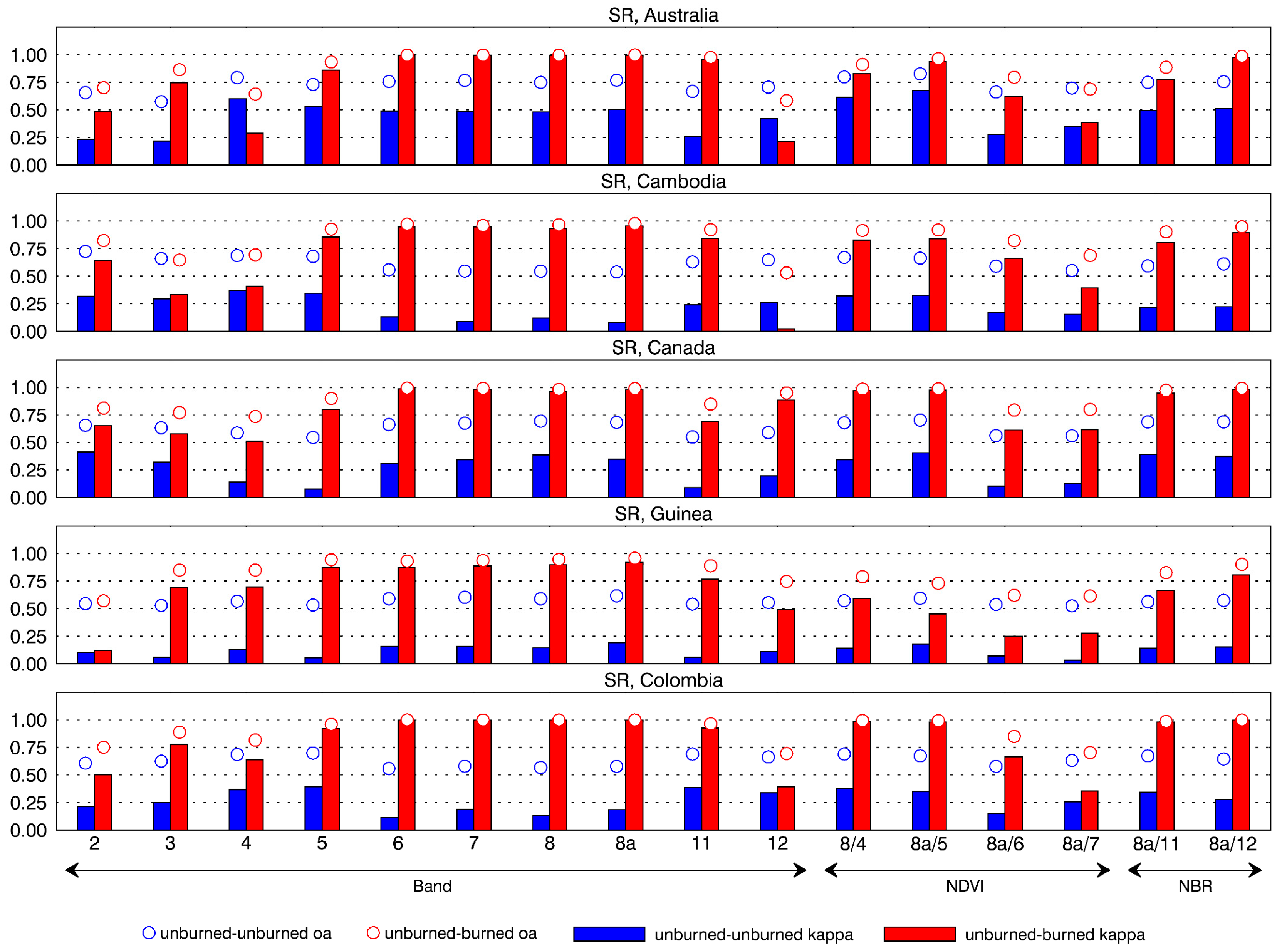
4. Results
5. Discussion
6. Conclusion
Acknowledgments
Author Contributions
Conflicts of Interest
References
- Giglio, L.; Descloitres, J.; Justice, C.O.; Kaufman, Y.J. An enhanced contextual fire detection algorithm for MODIS. Remote Sens. Environ. 2003, 87, 273–282. [Google Scholar] [CrossRef]
- Roy, D.P.; Boschetti, L.; Justice, C.O.; Ju, J. The collection 5 MODIS burned area product-Global evaluation by comparison with the MODIS active fire product. Remote Sens. Environ. 2008, 12, 3690–3707. [Google Scholar] [CrossRef]
- Xu, W.; Wooster, M.J.; Roberts, G.; Freeborn, P. New GOES imager algorithms for cloud and active fire detection and fire radiative power assessment across North, South and Central America. Remote Sens. Environ. 2010, 114, 1876–1895. [Google Scholar] [CrossRef]
- Zhang, X.; Kondragunta, S.; Ram, J.; Schmidt, C.; Huang, H.C. Near real time global biomass burning emissions product from geostationary satellite constellation. Geophys. Res. Atmos. 2012. [Google Scholar] [CrossRef]
- Mouillot, F.; Schultz, M.G.; Yue, C.; Cadule, P.; Tansey, K.; Ciais, P.; Chuvieco, E. Ten years of global burned area products from spaceborne remote sensing—A review: Analysis of user needs and recommendations for future developments. Int. J. Appl. Earth Obs. Geoinf. 2014, 26, 64–79. [Google Scholar] [CrossRef]
- Schroeder, W.; Oliva, P.; Giglio, L.; Csiszar, I.A. The new VIIRS 375 m active fire detection data product: Algorithm description and initial assessment. Remote Sens. Environ. 2014, 143, 85–96. [Google Scholar] [CrossRef]
- Alonso-Canas, I.; Chuvieco, E. Global burned area mapping from ENVISAT-MERIS and MODIS active fire data. Remote Sens. Environ. 2015, 163, 140–152. [Google Scholar] [CrossRef]
- Boschetti, L.; Roy, D.P.; Justice, C.O.; Humber, M.L. MODIS–Landsat fusion for large area 30 m burned area mapping. Remote Sens. Environ. 2015, 161, 27–42. [Google Scholar] [CrossRef]
- Drusch, M.; Del Bello, U.; Carlier, S.; Colin, O.; Fernandez, V.; Gascon, F.; Hoersch, B.; Isola, C.; Laberinti, P.; Martimort, P. Sentinel-2: ESA’s optical high-resolution mission for GMES operational services. Remote Sens. Environ. 2012, 120, 25–36. [Google Scholar] [CrossRef]
- Pereira, J.M.C. Remote sensing of burned areas in tropical savannas. Int. J. Wildland Fire 2003, 12, 259–270. [Google Scholar] [CrossRef]
- Trigg, S.N.; Roy, D.P.; Flasse, S.P. An in situ study of the effects of surface anisotropy on the remote sensing of burned savannah. Int. J. Remote Sens. 2005, 26, 4869–4876. [Google Scholar] [CrossRef]
- Roy, D.P.; Boschetti, L.; Maier, S.W.; Smith, A.M.S. Field estimation of ash and char color-lightness using a standard gray scale. Int. J. Wildland Fire 2010, 19, 698–704. [Google Scholar] [CrossRef]
- Lentile, L.B.; Holden, Z.A.; Smith, A.M.S.; Falkowski, M.J.; Hudak, A.T.; Morgan, P.; Lewis, S.A.; Gessler, P.E.; Benson, N.C. Remote sensing techniques to assess active fire characteristics and post-fire effects. Int. J. Wildland Fire 2006, 15, 319–345. [Google Scholar] [CrossRef]
- Roy, D.P.; Landmann, T. Characterizing the surface heterogeneity of fire effects using multi-temporal reflective wavelength data. Int. J. Remote Sens. 2005, 26, 4197–4218. [Google Scholar] [CrossRef]
- Pereira, J.M.C.; Chuvieco, E.; Beaudoin, A.; Desbois, N. Remote sensing of burned areas: A review. In A Review of Remote Sensing Methods for The Study of Large Wildland Fire Report of The Megafires Project ENV-CT96-0256; Chuvieco, E., Ed.; Universidad de Alcala: Alcala de Henares, Spain, 1997; pp. 127–183. [Google Scholar]
- Trigg, S.N.; Flasse, S.P. Characterizing the spectral-temporal response of burned savannah using in situ spectroradiometry and infrared thermometry. Int. J. Remote Sens. 2000, 21, 3161–3168. [Google Scholar] [CrossRef]
- Fraser, R.H.; Li, Z.; Landry, R. SPOT VEGETATION for characterizing boreal forest fires. Int. J. Remote Sens. 2000, 21, 3525–3532. [Google Scholar] [CrossRef]
- Jin, Y.; Roy, D.P. Fire-induced albedo change and its radiative forcing at the surface in northern Australia. Geophys. Res. Lett. 2005, 32, L13401. [Google Scholar] [CrossRef]
- Vila, J.P.S.; Barbosa, P. Post-fire vegetation regrowth detection in the Deiva Marina region (Liguria-Italy) using Landsat TM and ETM+ data. Ecol. Model. 2010, 221, 75–84. [Google Scholar] [CrossRef]
- Chu, T.; Guo, X.; Takeda, K. Remote sensing approach to detect post-fire vegetation regrowth in Siberian boreal larch forest. Ecol. Indic. 2016, 62, 32–46. [Google Scholar] [CrossRef]
- Smith, A.M.S.; Wooster, M.J.; Drake, N.A. Testing the potential of multi-spectral remote sensing for retrospectively estimating fire severity in African Savannahs. Remote Sens. Environ. 2005, 97, 92–115. [Google Scholar] [CrossRef]
- Stroppiana, D.; Pinnock, S.; Pereira, J.M.C.; Grégoire, J.-M. Radiometric analysis of SPOT-VEGETATION images for burnt area detection in Northern Australia. Remote Sens. Environ. 2002, 82, 21–37. [Google Scholar] [CrossRef]
- Roy, D.P.; Jin, Y.; Lewis, P.E.; Justice, C.O. Prototyping a global algorithm for systematic fire-affected area mapping using MODIS time series data. Remote Sens. Environ. 2005, 97, 137–162. [Google Scholar] [CrossRef]
- Kaufman, Y.J.; Hobbs, P.V.; Kirchhoff, V.W.J.H.; Artaxo, P.; Remer, L.A.; Holben, B.N.; King, M.D.; Ward, D.E.; Prins, E.M.; Longo, K.M.; et al. Smoke, Clouds, and Radiation-Brazil (SCAR-B) experiment. J. Geophys. Res. Atmos. 1998, 103, 31783–31808. [Google Scholar] [CrossRef]
- Lyapustin, A.; Wang, Y.; Laszlo, I.; Kahn, R.; Korkin, S.; Remer, L.; Levy, R.; Reid, J.S. Multiangle implementation of atmospheric correction (MAIAC): 2. Aerosol algorithm. J. Geophy. Res. Atmos. 2011. [Google Scholar] [CrossRef]
- Verstraete, M.M.; Pinty, B. Designing optimal spectral indexes for remote sensing applications. IEEE Trans. Geosci. Remote Sens. 1996, 34, 1254–1265. [Google Scholar] [CrossRef]
- Chuvieco, E.; Martín, M.P.; Palacios, A. Assessment of different spectral indices in the red-near-infrared spectral domain for burned land discrimination. Int. J. Remote Sens. 2002, 23, 5103–5110. [Google Scholar] [CrossRef]
- Chuvieco, E.; Riaño, D.; Danson, F.M.; Martin, P. Use of a radiative transfer model to simulate the postfire spectral response to burn severity. J. Geophys. Res. Biogeosci. 2006. [Google Scholar] [CrossRef]
- Levin, N.; Heimowitz, A. Mapping spatial and temporal patterns of Mediterranean wildfires from MODIS. Remote Sens. Environ. 2012, 126, 12–26. [Google Scholar] [CrossRef]
- Fernandez-Manso, A.; Fernandez-Manso, O.; Quintano, C. SENTINEL-2A red-edge spectral indices suitability for discriminating burn severity. Int. J. Appl. Earth Obs. Geoinf. 2016, 50, 170–175. [Google Scholar] [CrossRef]
- Liu, W.; Wang, L.; Zhou, Y.; Wang, S.; Zhu, J.; Wang, F. A comparison of forest fire burned area indices based on HJ satellite data. Nat. Hazards 2016, 81, 971–980. [Google Scholar] [CrossRef]
- Gao, F.; Jin, Y.; Schaaf, C.B.; Strahler, A.H. Bidirectional NDVI and atmospherically resistant BRDF inversion for vegetation canopy. IEEE Trans. Geosci. Remote Sens. 2002, 40, 1269–1278. [Google Scholar]
- Garcia, M.J.L.; Caselles, V. Mapping burns and natural reforestation using thematic Mapper data. Geocarto Int. 1991, 6, 31–37. [Google Scholar] [CrossRef]
- Loboda, T.; O’Neal, K.; Csiszar, I. Regionally adaptable dNBR-based algorithm for burned area mapping from MODIS data. Remote Sens. Environ. 2007, 109, 429–442. [Google Scholar] [CrossRef]
- Stroppiana, D.; Boschetti, M.; Zaffaroni, P.; Brivio, P. Analysis and interpretation of spectral indices for soft multicriteria burned-area mapping in mediterranean regions. IEEE Geosci. Remote Sens. Lett. 2009, 6, 499–503. [Google Scholar] [CrossRef]
- Veraverbeke, S.; Harris, S.; Hook, S. Evaluating spectral indices for burned area discrimination using MODIS/ASTER (MASTER) airborne simulator data. Remote Sens. Environ. 2011, 115, 2702–2709. [Google Scholar] [CrossRef]
- Davies, D.K.; Ilavajhala, S.; Wong, M.M.; Justice, C.O. Fire information for resource management system: Archiving and distributing MODIS active fire data. IEEE Trans. Geosci. Remote Sens. 2009, 47, 72–79. [Google Scholar] [CrossRef]
- Giglio, L.; Csiszar, I.; Justice, C.O. Global distribution and seasonality of active fires as observed with the Terra and Aqua Moderate Resolution Imaging spectroradiometer (MODIS) sensors. J. Geophys. Res. Biogeosci. 2006. [Google Scholar] [CrossRef]
- Friedl, M.A.; Sulla-Menashe, D.; Tan, B.; Schneider, A.; Ramankutty, N.; Sibley, A.; Huang, X. MODIS Collection 5 global land cover: Algorithm refinements and characterization of new datasets. Remote Sens. Environ. 2010, 114, 168–182. [Google Scholar] [CrossRef]
- Roy, D.P.; Li, J.; Zhang, H.K.; Yan, L. Best practices for the reprojection and resampling of Sentinel-2 Multi Spectral Instrument Level 1C data. Remote Sens. Lett. 2016, 7, 1023–1032. [Google Scholar] [CrossRef]
- Yan, L.; Roy, D.P.; Zhang, H.; Li, J.; Huang, H. An automated approach for sub-pixel registration of Landsat-8 Operational Land Imager (OLI) and Sentinel-2 Multi Spectral Instrument (MSI) imagery. Remote Sens. 2016, 8, 520. [Google Scholar] [CrossRef]
- Languille, F.; Déchoz, C.; Gaudel, A.; Greslou, D.; de Lussy, F.; Trémas, T.; Poulain, V. Sentinel-2 geometric image quality commissioning: First results. Proc. SPIE 2015. [Google Scholar] [CrossRef]
- Coppin, P.; Jonckheere, I.; Nackaerts, K.; Muys, B.; Lambin, E. Digital change detection methods in ecosystem monitoring: A review. Int. J. Remote Sens. 2004, 25, 1565–1596. [Google Scholar] [CrossRef]
- Kaufman, Y.J.; Sendra, C. Algorithm for automatic corrections to visible and near IR satellite imagery. Int. J. Remote Sens. 1988, 9, 1357–1381. [Google Scholar] [CrossRef]
- Tanre, D.; Herman, M.; Deschamps, P.Y. Influence of the background contribution upon space measurements of ground reflectance. Appl. Opt. 1981, 20, 3676–3684. [Google Scholar] [CrossRef] [PubMed]
- Chavez, P.S., Jr. Image-based atmospheric correction—Revisited and improved. Photogramm. Eng. Remote Sens. 1996, 62, 1025–1036. [Google Scholar]
- Müller-Wilm, U. Sentinel-2 MSI-Level-2A Prototype Processor Installation and User Manual; Telespazio VEGA Deutschland GmbH: Darmstadt, Germany, 2015. [Google Scholar]
- Claverie, M.; Vermote, E.; Franch, B.; He, T.; Hagolle, O.; Kadiri, M.; Masek, J. Evaluation of medium spatial resolution BRDF-Adjustment techniques using multi-angular SPOT4 (Take5) acquisitions. Remote Sens. 2015, 7, 12057–12075. [Google Scholar] [CrossRef]
- Roy, D.P.; Zhang, H.K.; Ju, J.; Gomez-Dans, J.L.; Lewis, P.E.; Schaaf, C.B.; Sun, Q.; Li, J.; Huang, H.; Kovalskyy, V. A general method to normalize Landsat reflectance data to nadir BRDF adjusted reflectance. Remote Sens. Environ. 2016, 176, 255–271. [Google Scholar] [CrossRef]
- Roy, D.P.; Frost, P.; Justice, C.; Landmann, T.; Le Roux, J.; Gumbo, K.; Makungwa, S.; Dunham, K.; Du Toit, R.; Mhwandagara, K.; et al. The Southern Africa Fire Network (SAFNet) regional burned area product validation protocol. Int. J. Remote Sens. 2005, 26, 4265–4292. [Google Scholar] [CrossRef]
- Boschetti, L.; Stehman, S.V.; Roy, D.P. A stratified random sampling design in space and time for regional to global scale burned area product validation. Remote Sens. Environ. 2016, 186, 465–478. [Google Scholar] [CrossRef]
- Jensen, J.R. Introductory Digital Image Processing: A Remote Sensing Perspective, 2nd ed.; Prentice Hall: Upper Saddle River, NJ, USA, 1996. [Google Scholar]
- Egorov, A.V.; Hansen, M.C.; Roy, D.P.; Kommareddy, A.; Potapov, P.V. Image interpretation-guided supervised classification using nested segmentation. Remote Sens. Environ. 2015, 165, 135–147. [Google Scholar] [CrossRef]
- Shapiro, S.S.; Wilk, M.B. An analysis of variance test for normality (complete samples). Biometrika 1965, 52, 591–611. [Google Scholar] [CrossRef]
- Mendes, M.; Pala, A. Type I error rate and power of three normality tests. Pak. J. Inform. Technol. 2003, 2, 135–139. [Google Scholar]
- Razali, N.M.; Wah, Y.B. Power comparisons of shapiro-wilk, kolmogorov-smirnov, lilliefors and anderson-darling tests. J. Stat. Model. Anal. 2011, 2, 21–33. [Google Scholar]
- Royston, P. Remark AS R94: A remark on algorithm AS181: The W-test for normality. J. R. Stat. Soc. Ser. 1995, 44, 547–551. [Google Scholar]
- Gómez, C.; White, J.C.; Wulder, M.A. Optical remotely sensed time series data for land cover classification: A review. ISPRS J. Photogramm. Remote Sens. 2016, 116, 55–72. [Google Scholar] [CrossRef]
- Breiman, L. Bagging predictors. Mach. Learn. 1996, 24, 123–140. [Google Scholar] [CrossRef]
- Breiman, L. Random forests. Mach. Learn. 2001, 45, 5–32. [Google Scholar] [CrossRef]
- Hothorn, T.; Hornik, K.; Zeileis, A. Unbiased recursive partitioning: A conditional inference framework. J. Comput. Graph. Stat. 2006, 15, 651–674. [Google Scholar] [CrossRef]
- Strobl, C.; Boulesteix, A.L.; Kneib, T.; Augustin, T.; Zeileis, A. Conditional variable importance for random forests. BMC Bioinform. 2008. [Google Scholar] [CrossRef] [PubMed] [Green Version]
- Foody, G.M. Status of land cover classification accuracy assessment. Remote Sens. Environ. 2002, 80, 185–201. [Google Scholar] [CrossRef]
- Ouaidrari, H.; Vermote, E.F. Operational atmospheric correction of Landsat TM data. Remote Sens. Environ. 1999, 70, 4–15. [Google Scholar] [CrossRef]
- Roy, D.P.; Qin, Y.; Kovalskyy, V.; Vermote, E.F.; Ju, J.; Egorov, A.; Hansen, M.C.; Kommareddy, I.; Yan, L. Conterminous United States demonstration and characterization of MODIS-based Landsat ETM+ atmospheric correction. Remote Sens. Environ. 2014, 140, 433–449. [Google Scholar] [CrossRef]
- Ju, J.; Roy, D.P.; Vermote, E.; Masek, J.; Kovalskyy, V. Continental-scale validation of MODIS-based and LEDAPS Landsat ETM+ atmospheric correction methods. Remote Sens. Environ. 2012, 122, 175–184. [Google Scholar] [CrossRef]
- Van Wagtendonk, J.W.; Root, R.R.; Key, C.H. Comparison of AVIRIS and Landsat ETM+ detection capabilities for burn severity. Remote Sens. Environ. 2004, 92, 397–408. [Google Scholar] [CrossRef]
- Koutsias, N.; Karteris, M. Logistic regression modelling of multitemporal Thematic Mapper data for burned area mapping. Int. J. Remote Sens. 1998, 19, 3499–3514. [Google Scholar] [CrossRef]
- Pereira, J.M.; Sá, A.C.; Sousa, A.M.; Silva, J.M.; Santos, T.N.; Carreiras, J.M. Spectral characterisation and discrimination of burnt areas. In Remote Sensing of Large Wildfires; Springer: Berlin, Germany, 1999; pp. 123–138. [Google Scholar]
- White, J.D.; Ryan, K.C.; Key, C.C.; Running, S.W. Remote sensing of forest fire severity and vegetation recovery. Int. J. Wildland Fire 1996, 6, 125–136. [Google Scholar] [CrossRef]
- Fraser, R.H.; Li, Z.; Cihlar, J. Hotspot and NDVI differencing synergy (HANDS): A new technique for burned area mapping over boreal forest. Remote Sens. Environ. 2000, 74, 362–376. [Google Scholar] [CrossRef]
- He, L.; Chen, J.M.; Zhang, S.; Gomez, G.; Pan, Y.; McCullough, K.; Masek, J.G. Normalized algorithm for mapping and dating forest disturbances and regrowth for the United States. Int. J. Appl. Earth Obs. Geoinf. 2011, 13, 236–245. [Google Scholar] [CrossRef]
- Dash, J.; Curran, P.J. The MERIS terrestrial chlorophyll index. Int. J. Remote Sens. 2004, 25, 5403–5413. [Google Scholar] [CrossRef]
- Clevers, J.G.; Gitelson, A.A. Remote estimation of crop and grass chlorophyll and nitrogen content using red-edge bands on Sentinel-2 and -3. Int. J. Appl. Earth Obs. Geoinf. 2013, 23, 344–351. [Google Scholar] [CrossRef]
- Roy, D.P.; Lewis, P.E.; Justice, C.O. Burned area mapping using multi-temporal moderate spatial resolution data—A bi-directional reflectance model-based expectation approach. Remote Sens. Environ. 2002, 83, 263–286. [Google Scholar] [CrossRef]
- Eva, H.; Lambin, E.F. Burnt area mapping in Central Africa using ATSR data. Int. J. Remote Sens. 1998, 19, 3473–3497. [Google Scholar] [CrossRef]
- Trigg, S.; Flasse, S. An evaluation of different bi-spectral spaces for discriminating burned shrub-savannah. Int. J. Remote Sens. 2001, 22, 2641–2647. [Google Scholar] [CrossRef]
- Chu, T.; Guo, X. Compositing MODIS time series for reconstructing burned areas in the Taiga–Steppe transition zone of northern Mongolia. Int. J. Wildland Fire 2015, 24, 419–432. [Google Scholar] [CrossRef]
- Fraser, R.H.; Li, Z. Estimating fire-related parameters in boreal forest using SPOT VEGETATION. Remote Sens. Environ. 2002, 82, 95–110. [Google Scholar] [CrossRef]
- Smith, A.M.S.; Drake, N.A.; Wooster, M.J.; Hudak, A.T.; Holden, Z.A.; Gibbons, C.J. Production of Landsat ETM+ reference imagery of burned areas within Southern African savannahs: comparison of methods and application to MODIS. Int. J. Remote Sens. 2007, 28, 2753–2775. [Google Scholar] [CrossRef]
- Lasaponara, R. Estimating spectral separability of satellite derived parameters for burned areas mapping in the Calabria region by using SPOT-Vegetation data. Ecol. Model. 2006, 196, 265–270. [Google Scholar] [CrossRef]
- Pereira, J.M.C. A comparative evaluation of NOAA/AVHRR vegetation indexes for burned surface detection and mapping. IEEE Trans. Geosci. Remote Sens. 1999, 37, 217–226. [Google Scholar] [CrossRef]
- Asner, G.P.; Heidebrecht, K.B. Spectral unmixing of vegetation, soil and dry carbon cover in arid regions: Comparing multispectral and hyperspectral observations. Int. J. Remote Sens. 2002, 23, 3939–3958. [Google Scholar] [CrossRef]
- Oliva, P.; Martín, P.; Chuvieco, E. Burned area mapping with MERIS post-fire image. Int. J. Remote Sens. 2011, 32, 4175–4201. [Google Scholar] [CrossRef]
- Gomez-Dans, J.L.; Lewis, P.E.; Disney, M. Efficient emulation of radiative transfer codes using Gaussian processes and application to land surface parameter inferences. Remote Sens. 2016, 8, 119. [Google Scholar] [CrossRef]
- Zhang, Y.H.; Wooster, M.J.; Tutubalina, O.; Perry, G.L.W. Monthly burned area and forest fire carbon emission estimates for the Russian Federation from SPOT VGT. Remote Sens. Environ. 2003, 87, 1–15. [Google Scholar] [CrossRef]
- Rogan, J.; Yool, S.R. Mapping fire-induced vegetation depletion in the Peloncillo Mountains Arizona and New Mexico. Int. J. Remote Sens. 2001, 22, 3101–3121. [Google Scholar] [CrossRef]
- Cocke, A.E.; Fule, P.Z.; Crouse, J.E. Comparison of burn severity assessments using differenced normalized burn ratio and ground data. Int. J. Wildland Fire 2005, 14, 189–198. [Google Scholar] [CrossRef]
- Epting, J.; Verbyla, D.; Sorbel, B. Evaluation of remotely sensed indices for assessing burn severity in interior Alaska using Landsat TM and ETM+. Remote Sens. Environ. 2005, 96, 328–339. [Google Scholar] [CrossRef]
- Roy, D.; Boschetti, L.; Trigg, S. Remote sensing of fire severity: Assessing the performance of the normalized burn ratio. IEEE Geosci. Remote Sens. Lett. 2006, 3, 112–116. [Google Scholar] [CrossRef]
- French, N.H.; Kasischke, E.S.; Hall, R.J.; Murphy, K.A.; Verbyla, D.L.; Hoy, E.E.; Allen, J.L. Using Landsat data to assess fire and burn severity in the North American boreal forest region: An overview and summary of results. Int. J. Wildland Fire 2008, 17, 443–462. [Google Scholar] [CrossRef]
- Schepers, L.; Haest, B.; Veraverbeke, S.; Spanhove, T.; Vanden Borre, J.; Goossens, R. Burned area detection and burn severity assessment of a heathland fire in Belgium using Airborne Imaging Spectroscopy (APEX). Remote Sens. 2014, 6, 1803–1826. [Google Scholar] [CrossRef]


| Site Location | L1C Tile ID | Acquisition Date 1 | Acquisition Date 2 | Predominant Vegetation Type |
|---|---|---|---|---|
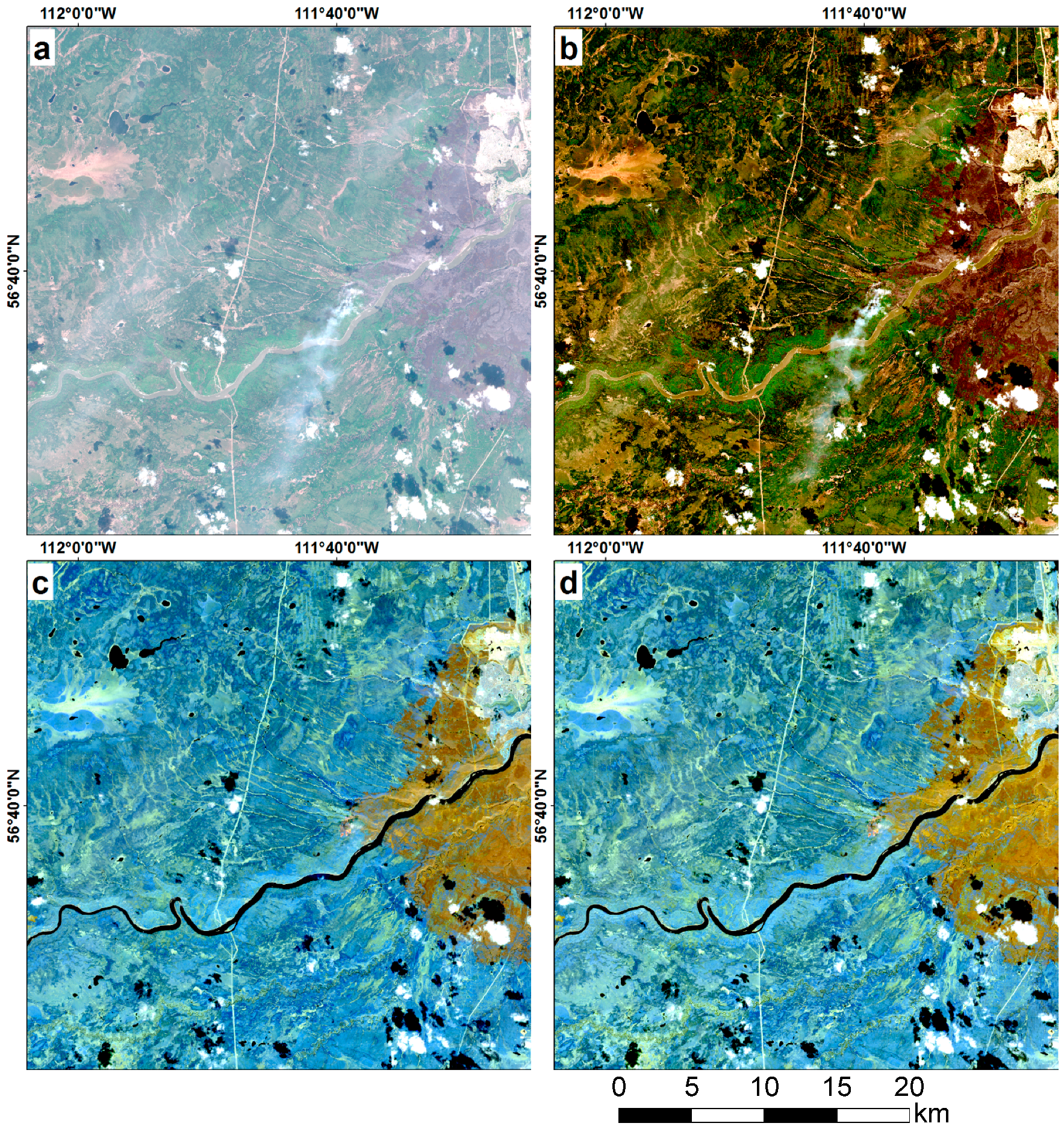
| Australia, Northern Territory, near Fish River Block Gorge National Park | 52LFK | 10 April 2016 | 30 April 2016 | Savannas |
| Cambodia, Kratié region, near Snoul | 48PXU | 7 January 2016 | 17 January 2016 | Woody savannas |
| Canada, Alberta, Fort McMurray | 12VVH | 2 May 2016 | 12 May 2016 | Evergreen needle leaf forest & Mixed forests |
| Guinea, Faranah Prefecture, Parc National du Haut Niger | 29PLM | 15 March 2016 | 25 March 2016 | Woody savannas |
| Colombia, Casanare Department, northern side of the Rio Cravo Sur river | 18NZL | 17 January 2016 | 6 Feburary 2016 | Savannas & Grassland |
| Sentinel-2 MSI Bands | Spatial Resolution (m) | Central Wavelength (nm) | Band Width (nm) |
|---|---|---|---|
| Band 1: Coastal Aerosol (b01) * | 60 | 443 | 20 |
| Band 2: Blue (b02) | 10 | 490 | 65 |
| Band 3: Green (b03) | 10 | 560 | 35 |
| Band 4: Red (b04) | 10 | 665 | 30 |
| Band 5: Vegetation Red Edge (b05) | 20 | 705 | 15 |
| Band 6: Vegetation Red Edge (b06) | 20 | 740 | 15 |
| Band 7: NIR (b07) | 20 | 783 | 20 |
| Band 8: NIR (b08) | 10 | 842 | 115 |
| Band 8A: NIR (b8a) | 20 | 865 | 20 |
| Band 9: Water Vapor (b09) * | 60 | 945 | 20 |
| Band 10: SWIR Cirrus (b10) * | 60 | 1375 | 30 |
| Band 11: SWIR (b11) | 20 | 1610 | 90 |
| Band 12: SWIR (b12) | 20 | 2190 | 180 |
| Spectral Index | Spatial Resolution (m) | Formulation |
|---|---|---|
| Normalized Difference Vegetation Index (8/4) | 10 | |
| Normalized Difference Vegetation Index red-edge (8a/5) | 20 | |
| Normalized Difference Vegetation Index red-edge (8a/6) | 20 | |
| Normalized Difference Vegetation Index (8a/7) | 20 | |
| Normalized Burn Ratio (8a/11) | 20 | |
| Normalized Burn Ratio (8a/12) | 20 |
| Site Location | Unburned to Burned | Unburned to Unburned |
|---|---|---|
| Australia, Northern Territory, near Fish River Block Gorge National Park | 8056 (0.81) | 8612 (0.86) |
| Cambodia, Kratié region, near Snoul | 8072 (0.81) | 8360 (0.84) |
| Canada, Alberta, Fort McMurray | 15,692 (1.57) | 14,124 (1.41) |
| Guinea, Faranah Prefecture, Parc National du Haut Niger | 8616 (0.86) | 8428 (0.84) |
| Colombia, Casanare Department, northern side of the Rio Cravo Sur river | 8316 (0.83) | 10,384 (1.04) |
| Reference Data | |||
|---|---|---|---|
| Class 1 | Class 2 | ||
| Classified Data | Class 1 | X11 | X12 |
| Class 2 | X21 | X22 | |
© 2016 by the authors; licensee MDPI, Basel, Switzerland. This article is an open access article distributed under the terms and conditions of the Creative Commons Attribution (CC-BY) license (http://creativecommons.org/licenses/by/4.0/).
Share and Cite
Huang, H.; Roy, D.P.; Boschetti, L.; Zhang, H.K.; Yan, L.; Kumar, S.S.; Gomez-Dans, J.; Li, J. Separability Analysis of Sentinel-2A Multi-Spectral Instrument (MSI) Data for Burned Area Discrimination. Remote Sens. 2016, 8, 873. https://0-doi-org.brum.beds.ac.uk/10.3390/rs8100873
Huang H, Roy DP, Boschetti L, Zhang HK, Yan L, Kumar SS, Gomez-Dans J, Li J. Separability Analysis of Sentinel-2A Multi-Spectral Instrument (MSI) Data for Burned Area Discrimination. Remote Sensing. 2016; 8(10):873. https://0-doi-org.brum.beds.ac.uk/10.3390/rs8100873
Chicago/Turabian StyleHuang, Haiyan, David P. Roy, Luigi Boschetti, Hankui K. Zhang, Lin Yan, Sanath Sathyachandran Kumar, Jose Gomez-Dans, and Jian Li. 2016. "Separability Analysis of Sentinel-2A Multi-Spectral Instrument (MSI) Data for Burned Area Discrimination" Remote Sensing 8, no. 10: 873. https://0-doi-org.brum.beds.ac.uk/10.3390/rs8100873