
Spaceborne Sun-Induced Vegetation Fluorescence Time Series from 2007 to 2015 Evaluated with Australian Flux Tower Measurements

 ,
,  , ,
, ,
Abstract
:
1. Introduction
2. SiF Retrieval Method and Setup
2.1. The GOME-2 Instrument
2.2. Forward Model
2.3. PC Analysis of Atmospheric Absorption Optical Thickness
2.4. Monthly SiF Maps
3. Seasonal Global Maps of Far-Red SiF Derived from GOME-2A
4. Evaluating Satellite-Retrieved Far-Red SiF with Data on Vegetation Activity
4.1. Comparison with NDVI
4.2. Comparing Far-Red SiF with GPP Derived from Australian Flux Tower Observations
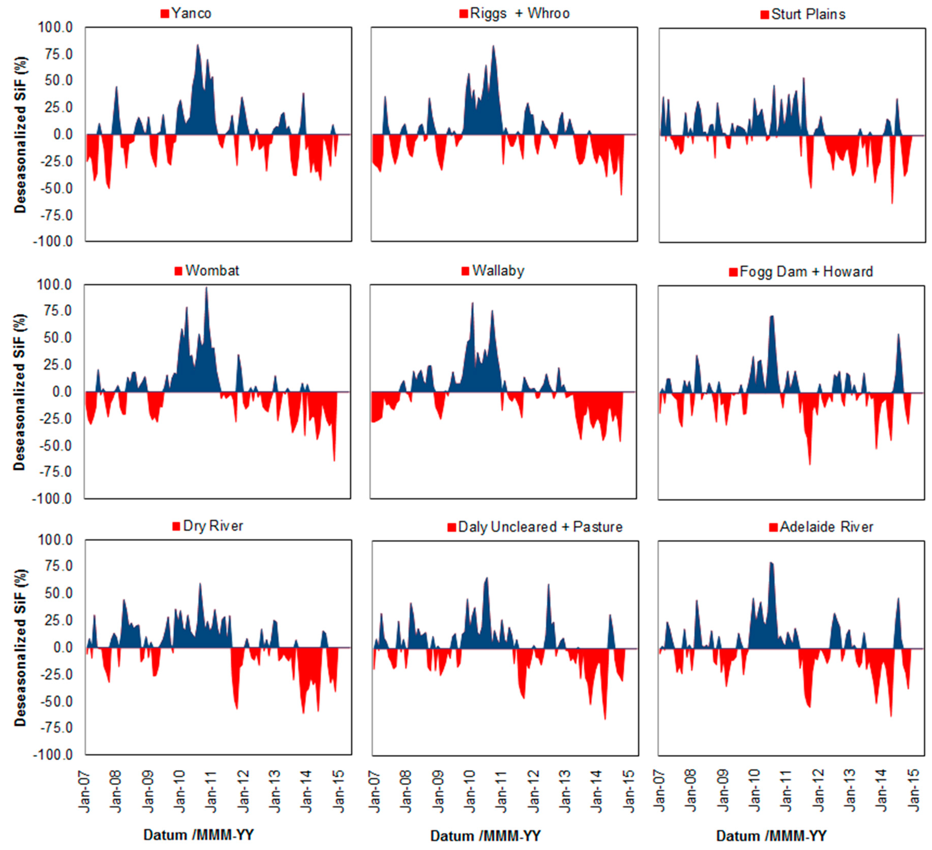
4.3. GOME-2A Retrieved SiF Time Series Analysis over Australian Flux Tower Sites: A Case Study
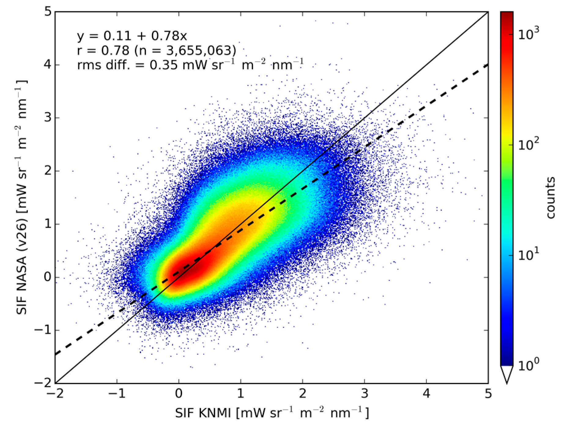
5. Comparison with SiF Retrieved from GOME-2A by Joiner et al. (2013)
6. Sensitivity Analyses for the Retrieval of GOME-2A SiF Using PCs
6.1. Number of PCs
6.2. Spectral Window
6.3. PC Reference Area
6.4. Conclusion of the Sensitivity Experiments
7. General Conclusions
Acknowledgments
Author Contributions
Conflicts of Interest
References
- Ciais, P.; Sabine, C.; Bala, G.; Bopp, L.; Brovkin, V.; Canadell, J.; Chhabra, A.; DeFries, R.; Galloway, J.; Heimann, M.; et al. Climate Change 2013: The Physical Science Basis. Contribution of Working Group I to the Fifth Assessment Report of the Intergovernmental Panel on Climate Change; Cambridge University Press: Cambridge, UK, 2013. [Google Scholar]
- Friedlingstein, P.; Cox, P.; Betts, R.; Bopp, L.; von Bloh, W.; Brovkin, V.; Doney, S.; Eby, M.; Fung, I.; Govindasamy, B.; et al. Climate-carbon cycle feedback analysis, results from the C4 26 MIP model intercomparison. J. Clim. 2006, 19, 3337–3353. [Google Scholar] [CrossRef]
- Piao, S.; Sitch, S.; Ciais, P.; Friedlingstein, P.; Peylin, P.; Wang, X.; Ahlström, A.; Anav, A.; Canadell, J.G.; Cong, N.; et al. Evaluation of terrestrial carbon cycle models for their response to climate variability and to CO2 trends. Glob. Chang. Biol. 2013. [Google Scholar] [CrossRef] [PubMed]
- Baldocchi, D.D.; Falge, E.; Gu, L.; Olson, R.; Hollinger, D.; Running, S.; Anthoni, P.; Bernhofer, C.; Davis, K.; Fuentes, J.; et al. FLUXNET: A new tool to study the temporal and spatial variability of ecosystem-scale carbon dioxide, water vapor, and energy flux densities. Bull. Am. Meteorol. Soc. 2001, 82, 2415–2435. [Google Scholar] [CrossRef]
- Desai, A.R.; Richardson, A.D.; Moffat, A.M.; Kattge, J.; Hollinger, D.Y.; Barr, A.; Falge, E.; Noormets, A.; Papale, D.; Reichstein, M.; et al. Cross-site evaluation of eddy covariance GPP and RE decomposition techniques. Agric. For. Meteorol. 2008, 148, 821–838. [Google Scholar] [CrossRef]
- Jung, M.; Reichstein, M.; Margolis, H.A.; Cescatti, A.; Richardson, A.D.; Arain, M.A.; Arneth, A.; Bernhofer, C.; Bonal, D.; Chen, J.Q.; et al. Global patterns of land-atmosphere fluxes of carbon dioxide, latent heat, and sensible heat derived from eddy covariance, satellite, and meteorological observations. J. Geophys. Res. 2011, 116, G00J07. [Google Scholar] [CrossRef]
- Pitman, J. The evolution of, and revolution in, land surface schemes designed for climate models. Int. J. Climatol. 2003, 23, 479–510. [Google Scholar] [CrossRef]
- Nemani, R.R.; Keeling, C.D.; Hashimoto, H.; Jolly, W.M.; Piper, S.C.; Tucker, C.J.; Myeni, R.B.; Running, S.W. Climate-driven increases in global terrestrial net primary production from 1982 to 1999. Science 2003, 300, 1560–1563. [Google Scholar] [CrossRef] [PubMed]
- Ryu, Y.; Baldocchi, D.D.; Kobayashi, H.; van Ingen, C.; Li, J.; Black, T.A.; Beringer, J.; van Gorsel, E.; Knohl, A.; Law, B.E.; et al. Integration of MODIS land and atmosphere products with a coupled-process model to estimate gross primary productivity and evapotranspiration from 1 km to global scales. Glob. Biogeochem. Cycles 2011, 25, B4017–B4017. [Google Scholar] [CrossRef]
- Kanniah, K.D.; Beringer, J.; Hutley, L.B. Response of savanna gross primary productivity to interannual variability in rainfall: Results of a remote sensing based light use efficiency model. Prog. Phys. Geogr. 2013, 37, 642–663. [Google Scholar] [CrossRef]
- Ma, X.; Huete, A.; Yu, Q.; Restrepo-Coupe, N.; Beringer, J.; Hutley, L.B.; Kanniah, K.D.; Cleverly, J.; Eamus, D. Parameterization of an ecosystem light-use-efficiency model for predicting savanna GPP using MODIS EVI. Remote Sens. Environ. 2014, 154, 253–271. [Google Scholar] [CrossRef]
- Rouse, J.W.; Haas, R.H.; Schell, J.A.; Deering, D.W. Monitoring Vegetation Systems in the Great Plains with ERTS; Third ERTS Symposium, NASA SP-351; NASA: Washington, DC, USA, 1973; pp. 309–317. [Google Scholar]
- Rouse, J.W.; Haas, R.H.; Schell, J.A.; Deering, D.W.; Harlan, J.C. Monitoring the Vernal Advancement and Retro-Gradation (Greenwave Effect) of Natural Vegetation; NASA/GSFC Type III Final Report; NASA: Greenbelt, MD, USA, 1974; p. 371. [Google Scholar]
- Tucker, C.J. Red and photographic infrared linear combinations for monitoring vegetation. Remote Sens. Environ. 1979, 8, 127–150. [Google Scholar] [CrossRef]
- Monteith, J. Solar-radiation and productivity in tropical ecosystems. J. Appl. Ecol. 1972, 9, 747–766. [Google Scholar] [CrossRef]
- Farquhar, G.; von Caemmerer, S.; Berry, J.A. A biochemical model of photosynthetic CO2 assimilation in leaves of C3 species. Planta 1980, 149, 78–90. [Google Scholar] [CrossRef] [PubMed]
- Veroustraete, F.; Sabbe, H.; Eerens, H. Estimation of carbon mass fluxes over Europe using the C-Fix model and Euroflux data. Remote Sens. Environ. 2002, 83, 376–399. [Google Scholar] [CrossRef]
- Schaefer, K.; Collatz, G.J.; Tans, P.P.; Denning, A.S.; Baker, I.; Berry, J.A.; Prihodko, L.; Suits, N.; Philpott, A. Combined simple biosphere/Carnegie-Ames-Stanford approach terrestrial carbon cycle model. J. Geophys. Res. 2008, 113, G03034. [Google Scholar] [CrossRef]
- Verstraeten, W.W.; Veroustraete, F.; Feyen, J. On temperature and water limitation of net ecosystem productivity: Implementation in the C-Fix model. Ecol. Model. 2006, 199, 4–22. [Google Scholar] [CrossRef]
- Verstraeten, W.W.; Veroustraete, F.; Wagner, W.; Van Roey, T.; Heyns, W.; Verbeiren, S.; Feyen, J. Impact assessment of remotely sensed soil moisture on ecosystem carbon fluxes across Europe. Clim. Chang. 2010, 103, 117–136. [Google Scholar] [CrossRef]
- Joiner, J.; Guanter, L.; Lindstrot, R.; Voigt, M.; Vasilkov, A.P.; Middleton, E.M.; Huemmrich, K.F.; Yoshida, Y.; Frankenberg, C. Global monitoring of terrestrial chlorophyll fluorescence from moderate-spectral-resolution near-infrared satellite measurements: Methodology, simulations, and application to GOME-2. Atmos. Meas. Tech. 2013, 6, 2803–2823. [Google Scholar] [CrossRef]
- Zhang, X.; Goldberg, M.; Tarpley, D.; Friedl, M.A.; Morisette, J.; Kogan, F.; Yu, Y. Drought-induced vegetation stress in southwestern North America. Environ. Res. Lett. 2010, 5, 024008. [Google Scholar] [CrossRef]
- Welp, L.R.; Keeling, R.F.; Meijer, H.A.J.; Bollenbacher, A.F.; Piper, S.C.; Yoshimura, K.; Francey, R.J.; Allison, C.E.; Wahlen, M. Interannual variability in the oxygen isotopes of atmospheric CO2 driven by El Nino. Nature 2011, 477, 579–582. [Google Scholar] [CrossRef] [PubMed]
- Kanniah, K.D.; Beringer, J.; Hutley, L.B. Environmental controls on the spatial variability of savanna productivity in the Northern Territory, Australia. Agric. For. Meteorol. 2011, 151, 1429–1439. [Google Scholar] [CrossRef]
- Pedros, R.; Moya, I.; Goulas, Y.; Jacquemoud, S. Chlorophyll fluorescence emission spectrum inside a leaf. Photochem. Photobiol. Sci. 2008, 7, 498–502. [Google Scholar] [CrossRef] [PubMed]
- Guanter, L.; Rossini, M.; Colombo, R.; Meroni, M.; Frankenberg, C.; Lee, J.-E.; Joiner, J. Using field spectroscopy to assess the potential of statistical approaches for the retrieval of sun-induced chlorophyll fluorescence from ground and space. Remote Sens. Environ. 2013, 133, 52–61. [Google Scholar] [CrossRef]
- Zarco-Tejada, P.J.; González-Dugo, V.; Berni, J.A.J. Fluorescence, temperature and narrow-band indices acquired from a UAV platform for water stress detection using a micro-hyperspectral imager and a thermal camera. Remote Sens. Environ. 2012, 117, 322–337. [Google Scholar] [CrossRef]
- Meroni, M.; Rossini, M.; Guanter, L.; Alonso, L.; Rascher, U.; Colombo, R.; Moreno, J. Remote sensing of solar-induced chlorophyll fluorescence: Review of methods and applications. Remote Sens. Environ. 2009, 113, 2037–2051. [Google Scholar] [CrossRef]
- Baker, N.R. Chlorophyll fluorescence: A probe of photosynthesis in vivo. Ann. Rev. Plant Biol. 2008, 59, 89–113. [Google Scholar] [CrossRef] [PubMed]
- Sanders, A.F.J.; De Haan, J.F. Retrieval of aerosol parameters from the oxygen A band in the presence of chlorophyll fluorescence. Atmos. Meas. Tech. 2013, 6, 2725–2740. [Google Scholar] [CrossRef]
- Frankenberg, C.; O’Dell, C.; Guanter, L.; McDuffie, J. Remote sensing of near-infrared chlorophyll fluorescence from space in scattering atmospheres: Implications for its retrieval and interferences with atmospheric CO2 retrievals. Atmos. Meas. Tech. 2012, 5, 2081–2094. [Google Scholar] [CrossRef]
- Joiner, J.; Yoshida, Y.; Vasilkov, A.P.; Yoshida, Y.; Corp, L.A.; Middleton, E.M. First observations of global and seasonal terrestrial chlorophyll fluorescence from space. Biogeosciences 2011, 8, 637–651. [Google Scholar] [CrossRef] [Green Version]
- Joiner, J.; Yoshida, Y.; Vasilkov, A.P.; Middleton, E.M.; Campbell, P.K.E.; Yoshida, Y.; Kuze, A.; Corp, L.A. Filling-in of near-infrared solar lines by terrestrial fluorescence and other geophysical effects: Simulations and space-based observations from SCIAMACHY and GOSAT. Atmos. Meas. Tech. 2012, 5, 809–829. [Google Scholar] [CrossRef]
- Frankenberg, C.; Fisher, J.B.; Worden, J.; Badgley, G.; Saatchi, S.S.; Lee, J.-E.; Toon, G.C.; Butz, A.; Jung, M.; Kuze, A.; et al. New global observations of the terrestrial carbon cycle from GOSAT: Patterns of plant fluorescence with gross primary productivity. Geophys. Res. Lett. 2011, 38, L17706. [Google Scholar] [CrossRef]
- Guanter, L.; Frankenberg, C.; Dudhia, A.; Lewis, P.E.; Gómez-Dans, J.; Kuze, A.; Suto, H.; Grainger, R.G. Retrieval and global assessment of terrestrial chlorophyll fluorescence from GOSAT space measurements. Remote Sens. Environ. 2012, 121, 236–251. [Google Scholar] [CrossRef]
- Köhler, P.; Guanter, L.; Joiner, J. A linear method for the retrieval of sun-induced chlorophyll fluorescence from GOME-2 and SCIAMACHY Data. Atmos. Meas. Tech. 2015, 8, 2589–2608. [Google Scholar]
- Khosravi, N.; Vountas, M.; Rozanov, V.V.; Bracher, A.; Wolanin, A.; Burrows, J.P. Retrieval of terrestrial plant fluorescence based on the in-filling of far-red Fraunhofer lines using SCIAMACHY observations. Front. Environ. Sci. 2015, 3, 78. [Google Scholar] [CrossRef] [Green Version]
- Frankenberg, C.; O’Dell, C.; Berry, J.; Guanter, L.; Joiner, J.; Köhler, P.; Pollock, R.; Taylor, T.E. Prospects for chlorophyll fluorescence remote sensing from the Orbiting Carbon Observatory-2. Remote Sens. Environ. 2014, 147, 1–12. [Google Scholar] [CrossRef]
- Guanter, L.; Aben, I.; Tol, P.; Krijger, J.M.; Hollstein, A.; Köhler, P.; Damm, A.; Joiner, J.; Frankenberg, C.; Landgraf, J. Potential of the TROPOspheric Monitoring Instrument (TROPOMI) onboard the Sentinel-5 Precursor for the monitoring of terrestrial chlorophyll fluorescence. Atmos. Meas. Tech. 2015, 8, 1337–1352. [Google Scholar] [CrossRef]
- Kraft, S.; Del Bello, U.; Bouvet, M.; Drusch, M.; Moreno, J. FLEX: ESA’s Earth Explorer 8 candidate mission. In Proceedings of 2012 IEEE International Geoscience and Remote Sensing Symposium, Munich, Germany, 22–27 July 2012; pp. 7125–7128.
- Guanter, L.; Alonso, L.; Gómez-Chova, L.; Amorós-López, J.; Vila, J.; Moreno, J. Estimation of solar-induced vegetation fluorescence from space measurements. Geophys. Res. Lett. 2007, 34, L08401. [Google Scholar] [CrossRef]
- Guanter, L.; Alonso, L.; Gómez-Chova, L.; Meroni, M.; Preusker, R.; Fischer, J.; Moreno, J. Developments for vegetation florescence retrieval from spaceborne high-resolution spectrometry in the O2-A and O2-B absorption bands. J. Geophys. Res. 2010, 115, D19303. [Google Scholar] [CrossRef]
- Frankenberg, C.; Butz, A.; Toon, G.C. Disentangling chlorophyll fluorescence from atmospheric scattering effects in O2 A-band spectra of reflected sun-light. Geophys. Res. Lett. 2011, 38, L03801. [Google Scholar] [CrossRef]
- Van der Tol, C.; Verhoef, W.; Rosema, A. A model for chlorophyll fluorescence and photosynthesis at leaf scale. Agric. For. Meteorol. 2009, 149, 96–105. [Google Scholar] [CrossRef]
- Damm, A.; Erler, A.; Hillen, W.; Meroni, M.; Schaepman, M.E.; Verhoef, W.; Rascher, U. Far-red sun-induced chlorophyll fluorescence shows ecosystem-specific relationships to gross primary production: An assessment based on observational and modeling approaches. Remote Sens. Environ. 2015, 115, 1882–1892. [Google Scholar] [CrossRef]
- Lee, J.-E.; Frankenberg, C.; van der Tol, C.; Berry, J.A.; Guanter, L.; Boyce, C.K.; Fisher, J.B.; Morrow, E.; Worden, J.R.; Asefi, S.; et al. Forest productivity and water stress in Amazonia: Observations from GOSAT chlorophyll fluorescence. Proc. R. Soc. B Biol. Sci. 2013. [Google Scholar] [CrossRef] [PubMed]
- Damm, A.; Elbers, J.; Erler, A.; Gioli, B.; Hamdi, K.; Hutjes, R.; Kosvancova, M.; Meroni, M.; Miglietta, F.; Moersch, A.; et al. Remote sensing of sun-induced fluorescence to improve modeling of diurnal courses of gross primary production (GPP). Glob. Chang. Biol. 2010, 16, 171–186. [Google Scholar] [CrossRef] [Green Version]
- Wagle, P.; Zhang, Y.; Jin, C.; Xiao, X. Comparison of solar-induced chlorophyll fluorescence, light-use efficiency, and process-based GPP models in maize. Ecol. Appl. 2016, 26, 1211–1222. [Google Scholar] [CrossRef] [PubMed]
- Yang, X.; Tang, J.; Mustard, J.F.; Lee, J.E.; Rossini, M.; Joiner, J.; Munger, J.W.; Kornfeld, A.; Richardson, A.D. Solar-induced chlorophyll fluorescence that correlates with canopy photosynthesis on diurnal and seasonal scales in a temperate deciduous forest. Geophys. Res. Lett. 2015, 42, 2977–2987. [Google Scholar] [CrossRef]
- Zhang, Y.; Xiao, X.; Jin, C.; Dong, J.; Zhou, S.; Wagle, P.; Joiner, J.; Guanter, L.; Zhang, Y.; Zhang, G. Consistency between sun-induced chlorophyll fluorescence and gross primary production of vegetation in North America. Remote Sens. Environ. 2016, 183, 154–169. [Google Scholar] [CrossRef]
- Rossini, M.; Meroni, M.; Celesti, M.; Cogliati, S.; Julitta, T.; Panigada, C.; Rascher, U.; van der Tol, C.; Colombo, R. Analysis of red and far-red sun-induced chlorophyll fluorescence and their ratio in different canopies based on observed and modeled data. Remote Sens. 2016, 8, 412. [Google Scholar] [CrossRef]
- Porcar-Castell, A.; Tyystjärvi, E.; Atherton, J.; van der Tol, C.; Flexas, J.; Pfündel, E.E.; Moreno, J.; Frankenberg, C.; Berry, J.A. Linking chlorophyll a fluorescence to photosynthesis for remote sensing applications: Mechanisms and challenges. J. Exp. Bot. 2014, 65, 4065–4095. [Google Scholar] [CrossRef] [PubMed]
- Guanter, L.; Zhang, Y.; Jung, M.; Joiner, J.; Voigt, M.; Berry, J.A.; Frankenberg, C.; Huete, A.R.; Zarco-Tejada, P.; Lee, J.-E.; et al. Global and time-resolved monitoring of crop photosynthesis with chlorophyll fluorescence. Proc. Natl. Acad. Sci. USA 2014, 111, E1327–E1333. [Google Scholar] [CrossRef] [PubMed]
- Joiner, J.; Yoshida, Y.; Vasilkov, A.P.; Schaefer, K.; Jung, M.; Guanter, L.; Zhang, Y.; Garrity, S.; Middleton, E.M.; Huemmrich, K.F.; et al. The seasonal cycle of satellite chlorophyll fluorescence observations and its relationship to vegetation phenology and ecosystem atmosphere carbon exchange. Remote Sens. Environ. 2014, 152, 375–391. [Google Scholar] [CrossRef]
- Callies, J.; Corpaccioli, E.; Eisinger, M.; Hahne, A.; Lefebvre, A. GOME-2—MetOp’s second generation sensor for operational ozone monitoring. ESA Bull. 2000, 102, 28–36. [Google Scholar]
- Thomas, G.E.; Stamnes, K. Radiative Transfer in the Atmosphere and Ocean; Cambridge University Press: Cambridge, UK, 2002. [Google Scholar]
- Zarco-Tejada, P.J.; Miller, J.R.; Mohammed, G.H.; Noland, T.L. Chlorophyll fluorescence effects on vegetation apparent reflectance: I. Leaf-level measurements and model simulation. Remote Sens. Environ. 2000, 74, 582–595. [Google Scholar] [CrossRef]
- Chance, K.; Kurucz, R.L. An improved high-resolution solar reference spectrum for earth’s atmosphere measurements in the ultraviolet, visible, and near infrared. J. Quant. Spectrosc. Radiat. 2010, 111, 1289–1295. [Google Scholar] [CrossRef]
- Joiner, J.; Yoshida, Y.; Guanter, L.; Middleton, E.M. New methods for retrieval of chlorophyll red fluorescence from hyper-spectral satellite instruments: Simulations and application to GOME-2 and SCIAMACHY. Atmos. Meas. Tech. 2016, 9, 3939–3967. [Google Scholar] [CrossRef]
- Koelemeijer, R.B.A.; Stammes, P.; Hovenier, J.W.; De Haan, J.F. A fast method for retrieval of cloud parameters using oxygen A band measurements from the Global Ozone Monitoring Experiment. J. Geophys. Res. 2001, 106, 3475–3490. [Google Scholar] [CrossRef] [Green Version]
- Wang, P.; Stammes, P.; van der A, R.; Pinardi, G.; van Roozendael, M. FRESCO+: An improved O2 A-band cloud retrieval algorithm for tropospheric trace gas retrievals. Atmos. Chem. Phys. 2008, 8, 6565–6576. [Google Scholar] [CrossRef]
- Wold, H. Estimation of Principal Components and related models by iterative least squares. In Multivariate Analysis; Krishnaiah, P.R., Ed.; Academic Press: New York, NY, USA, 1966. [Google Scholar]
- Wold, H. Nonlinear Iterative Partial Least Squares (NIPALS) modeling: Some current developments. In Multivariate Analysis II, Proceedings of the International Symposium on Multivariate Analysis, Wright State University, Dayton, OH, USA; Krishnaiah, P.R., Ed.; Academic Press: New York, NY, USA, 1973. [Google Scholar]
- Moya, I.; Camenen, L.; Evain, S.; Goulas, Y.; Cerovic, Z.G.; Latouche, G.; Flexas, J.; Ounis, A. A new instrument for passive remote sensing 1. Measurements of sunlight-induced chlorophyll fluorescence. Remote Sens. Environ. 2004, 91, 186–197. [Google Scholar] [CrossRef]
- Rossini, M.; Meroni, M.; Migliavacca, M.; Manca, G.; Cogliati, S.; Busetto, L.; Picchi, V.; Cescatti, A.; Seufert, G.; Colombo, R. High resolution field spectroscopy measurements for estimating gross ecosystem production in a rice field. Agric. For. Meteorol. 2010, 150, 1283–1296. [Google Scholar] [CrossRef]
- Drolet, G.G.; Wade, T.; Nichol, C.J.; MacLellan, C.; Levula, J.; Porcar-Castell, A.; Nikinmaa, E.; Vesala, T. A temperature-controlled spectrometer system for continuous and unattended measurements of canopy spectral radiance and reflectance. Int. J. Remote Sens. 2014, 35, 1769–1785. [Google Scholar] [CrossRef]
- Zarco-Tejada, P.J.; Berni, J.A.; Suárez, L.; Sepulcre-Cantó, G.; Morales, F.; Miller, J. Imaging chlorophyll fluorescence with an airborne narrow-band multispectral camera for vegetation stress detection. Remote Sens. Environ. 2009, 113, 1262–1275. [Google Scholar] [CrossRef]
- Zarco-Tejada, P.J.; Catalina, A.; González, M.; Martín, P. Relationships between net photosynthesis and steady-state chlorophyll fluorescence retrieved from airborne hyperspectral imagery. Remote Sens. Environ. 2013, 136, 247–258. [Google Scholar] [CrossRef]
- Morton, D.C.; Nagol, J.; Carabajal, C.C.; Rosette, J.; Palace, M.; Cook, B.D.; Vermote, E.F.; Harding, D.J.; North, P.R. Amazon forests maintain consistent canopy structure and greenness during the dry season. Nature 2014, 506, 221–224. [Google Scholar] [CrossRef] [PubMed]
- Haboudane, D.; Miller, J.R.; Tremblay, N.; Zarco-Tejada, P.J.; Dextraze, L. Integrated narrow-band vegetation indices for prediction of crop chlorophyll content for application to precision agriculture. Remote Sens. Environ. 2002, 81, 416–426. [Google Scholar] [CrossRef]
- Donohue, R.J.; Hume, I.H.; Roderick, M.L.; McVicar, T.R.; Beringer, J.; Hutley, L.B.; Gallant, J.C.; Austin, J.M.; van Gorsel, E.; Cleverly, J.R.; et al. Evaluation of the remote-sensing-based DIFFUSE model for estimating photosynthesis of vegetation. Remote Sens. Environ. 2014, 155, 349–365. [Google Scholar] [CrossRef]
- Beringer, J.; Hutley, L.B.; McHugh, I.; Arndt, S.K.; Campbell, D.; Cleugh, H.A.; Cleverly, J.; Resco de Dios, V.; Eamus, D.; Evans, B.; et al. An introduction to the Australian and New Zealand flux tower network—OzFlux. Biogeosci. Discuss. 2016. in preparation for OzFlux Special Issue. [Google Scholar] [CrossRef]
- Beringer, J.; Hutley, L.B.; Hacker, J.M.; Neininger, B.; Tha Paw, U.K. Patterns and processes of carbon, water and energy cycles across northern Australian landscapes: From point to region. Agric. For. Meteorol. 2011, 151, 1409–1416. [Google Scholar] [CrossRef]
- Hutley, L.B.; Beringer, J.; Isaac, P.R.; Hacker, J.M.; Cernusak, L. A sub-continental scale living laboratory: Spatial patterns of savanna vegetation over a rainfall gradient in northern Australia. Agric. For. Meteorol. 2011, 151, 1417–1428. [Google Scholar] [CrossRef]
- Van der Tol, C.; Berry, J.A.; Campbell, P.K.E.; Rascher, U. Models of fluorescence and photosynthesis for interpreting measurements of solar-induced chlorophyll fluorescence. Journal of Geophysical Research. Biogeosciences 2014, 119, 2312–2327. [Google Scholar] [PubMed]
- Cai, W.; Purich, A.; Cowan, T.; van Rensch, P.; Weller, E. Did climate change-induced rainfall trends contribute to the Australian millennium drought? J. Clim. 2014, 27, 3145–3168. [Google Scholar] [CrossRef]
- Australian Bureau of Meteorology. Record-Breaking La Niña Events: An Analysis of the La Niña Life Cycle and the Impacts and Significance of the 2010–2011 and 2011–2012 La Niña Events in Australia; Published by the Bureau of Meteorology, July 2012. Available online: http://www.bom.gov.au (accessed on 16 November 2015).
- Poulter, B.; Frank, D.; Ciais, P.; Myneni, R.B.; Andela, A.; Bi, J.; Broquet, G.; Canadell, J.G.; Chevallier, F.; Liu, Y.Y.; et al. Contribution of semi-arid ecosystems to interannual variability of the global carbon cycle. Nature 2014, 509, 600–603. [Google Scholar] [CrossRef] [PubMed]
- Ahlström, A.; Raupach, M.R.; Schurgers, G.; Smith, B.; Arneth, A.; Jung, M.; Reichstein, M.; Canadell, J.G.; Friedlingstein, P.; Jain, A.K.; et al. Carbon cycle. The dominant role of semi-arid ecosystems in the trend and variability of the land CO2 sink. Science 2015, 348, 895–899. [Google Scholar] [CrossRef] [PubMed]
- Haverd, V.; Smith, B.; Trudinger, C. Dryland vegetation response to wet episode, not inherent shift in sensitivity to rainfall, behind Australia’s role in 2011 global carbon sink anomaly. Glob. Chang. Biol. 2015. [Google Scholar] [CrossRef] [PubMed]
- Sun, Y.; Fu, R.; Dickinson, R.; Joiner, J.; Frankenberg, C.; Gu, L.; Xia, Y.; Fernando, N. Drought onset mechanisms revealed by satellite solar-induced chlorophyll fluorescence: Insights from two contrasting extreme events. J. Geophys. Res. Biogeosci. 2015, 120, 2427–2440. [Google Scholar] [CrossRef]
- Yoshida, Y.; Joiner, J.; Tucker, C.J.; Berry, J.; Lee, J.-L.; Walker, G.; Reichle, R.; Koster, R.; Lyapustin, A.; Wang, Y. The 2010 Russian drought impact on satellite measurements of solar-induced chlorophyll fluorescence: Insights from modeling and comparisons with parameters derived from satellite reflectances. Remote Sens. Environ. 2015, 166, 163–177. [Google Scholar] [CrossRef]


| Site Name | Latitude (S)/Longitude (E) | Vegetation |
|---|---|---|
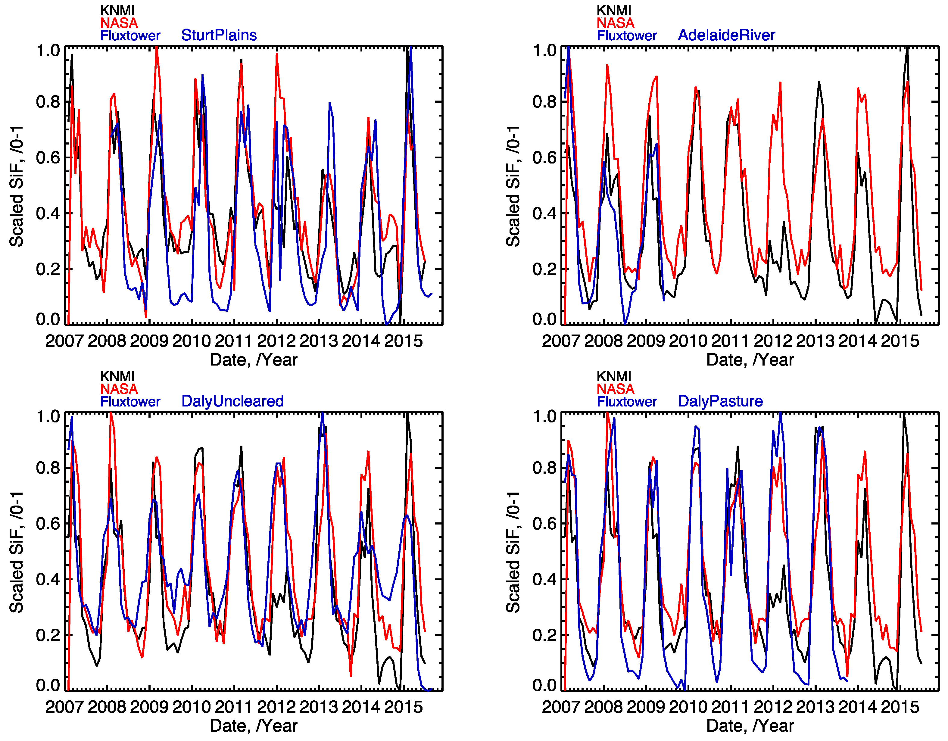
| Sturt Plains | 17°9′2′′, 133°21′1′′ | Grassland |
| Daly Uncleared | 14°09′33′′, 131°23′17′′ | Woodland savannah |
| Adelaide River | 13°4′37′′, 131°7′4′′ | Woodland savannah |
| Daly Pasture | 14°03′48′′, 131°19′05′′ | Tropical pasture |
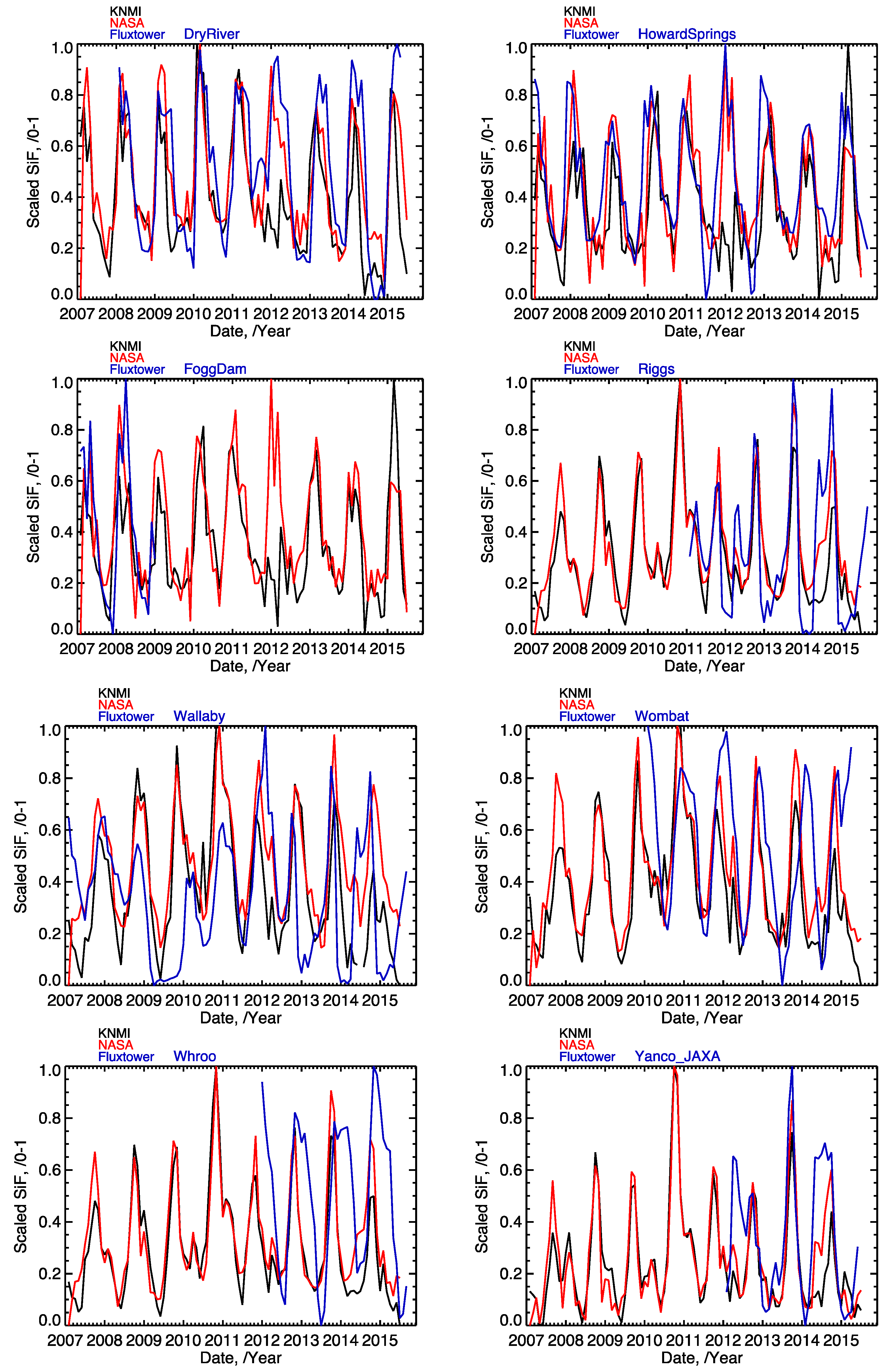
| Dry River | 15°15′32′′, 132°22′14′′ | Woodland savannah |
| Fogg Dam | 12°32′42′′, 131°18′26′′ | Flooded wetland |
| Howard Springs | 12°29′42′′, 131°09′00′′ | Open-forest savannah |
| Riggs | 36°39′00′′, 145°34′34′′ | Dryland agriculture (pasture) |
| Wallaby | 37°25′34′′, 145°11′14′′ | Eucalyptus forest |
| Whroo | 36°40′23′′, 145°01′34′′ | Box woodland |
| Wombat | 37°25′20′′, 144°05′40′′ | Secondary forest |
| Yanco Jaxa | 34°59′16′′, 146°17′27′′ | Dryland agriculture (pasture) |
| GOME-2 SIF KNMI vs. Flux Tower GPP | GOME-2 SIF NASA (v26) vs. Flux Tower GPP | |||||
|---|---|---|---|---|---|---|
| Slope | Intercept | R | Slope | Intercept | R | |
| Sturt Plains | 11.5 | −3.0 | 0.739 | 13.4 | −2.0 | 0.776 |
| Daly Uncleared | 7.9 | 2.5 | 0.699 | 8.6 | 3.4 | 0.637 |
| Adelaide River | 17.5 | −1.7 | 0.835 | 12.6 | 3.0 | 0.691 |
| Daly Pasture | 20.0 | −6.0 | 0.831 | 24.0 | −4.4 | 0.871 |
| Dry River | 5.4 | 4.0 | 0.622 | 8.4 | 3.4 | 0.821 |
| Fogg Dam | 12.1 | −0.2 | 0.763 | 7.0 | 3.6 | 0.554 |
| Howard Springs | 12.2 | 5.1 | 0.554 | 15.0 | 6.4 | 0.646 |
| Riggs | 8.2 | −1.0 | 0.627 | 11.8 | −1.0 | 0.781 |
| Wallaby | 3.7 | 4.0 | 0.265 | 7.6 | 3.0 | 0.366 |
| Whroo | 2.5 | 5.0 | 0.371 | 2.2 | 5.8 | 0.299 |
| Wombat | 4.4 | 8.6 | 0.397 | 6.8 | 8.7 | 0.433 |
| Yanco Jaxa | 4.4 | 0.0 | 0.570 | 6.5 | 0.3 | 0.800 |
| All | 6.8 | 2.8 | 0.456 | 9.7 | 2.9 | 0.510 |
| Number of PCs | Month | RMS | Mean | STD | R | Slope | Intercept | N |
|---|---|---|---|---|---|---|---|---|
| 15 | January | 0.85 | −0.11 | 0.85 | 0.67 | 0.39 | 0.44 | 28,844 |
| April | 0.80 | 0.54 | 0.59 | 0.83 | 0.39 | 0.00 | 37,706 | |
| July | 1.52 | 1.00 | 1.14 | 0.85 | 0.29 | 0.16 | 44,326 | |
| October | 0.74 | 0.32 | 0.67 | 0.79 | 0.40 | 0.13 | 40,786 | |
| All | 1.06 | 0.49 | 0.94 | 0.74 | 0.32 | 0.19 | 151,662 | |
| 25 | January | 0.20 | 0.09 | 0.18 | 0.99 | 0.82 | 0.04 | 28,844 |
| April | 0.25 | 0.19 | 0.16 | 0.97 | 0.76 | −0.06 | 37,706 | |
| July | 0.90 | 0.69 | 0.58 | 0.94 | 0.48 | 0.00 | 44,328 | |
| October | 0.51 | 0.34 | 0.39 | 0.95 | 0.58 | −0.01 | 40,786 | |
| All | 0.57 | 0.36 | 0.45 | 0.92 | 0.56 | 0.03 | 151,664 | |
| 45 | January | 0.15 | −0.06 | 0.13 | 0.99 | 1.13 | −0.01 | 28,844 |
| April | 0.18 | 0.09 | 0.15 | 0.97 | 0.78 | 0.01 | 37,706 | |
| July | 0.17 | 0.11 | 0.13 | 0.99 | 0.84 | 0.01 | 44,328 | |
| October | 0.22 | 0.12 | 0.18 | 0.98 | 0.77 | 0.01 | 40,786 | |
| All | 0.18 | 0.07 | 0.17 | 0.97 | 0.86 | 0.01 | 151,664 |
| Spectral Window | Month | RMS | Mean | STD | R | Slope | Intercept | N |
|---|---|---|---|---|---|---|---|---|
| 734–758 nm (FH) | January | 1.16 | −0.11 | 1.15 | 0.45 | 0.23 | 0.53 | 28,805 |
| April | 0.41 | −0.08 | 0.40 | 0.74 | 0.51 | 0.21 | 37,677 | |
| July | 0.43 | −0.09 | 0.42 | 0.72 | 0.67 | 0.27 | 44,297 | |
| October | 1.58 | −0.19 | 1.57 | 0.22 | 0.07 | 0.41 | 40,592 | |
| All | 1.01 | −0.12 | 1.00 | 0.42 | 0.21 | 0.43 | 151,371 | |
| 712–758 nm (H2O, FH) | January | 0.41 | 0.02 | 0.41 | 0.91 | 0.67 | 0.20 | 28,813 |
| April | 0.57 | 0.25 | 0.51 | 0.85 | 0.43 | 0.09 | 37,700 | |
| July | 0.46 | 0.21 | 0.41 | 0.93 | 0.59 | 0.15 | 44,325 | |
| October | 0.33 | 0.04 | 0.33 | 0.95 | 0.62 | 0.13 | 40,761 | |
| All | 0.45 | 0.14 | 0.43 | 0.90 | 0.58 | 0.13 | 151,599 | |
| 734–783 nm (FH, O2 A) | January | 0.46 | −0.28 | 0.37 | 0.88 | 1.48 | 0.10 | 28,844 |
| April | 0.21 | −0.03 | 0.21 | 0.86 | 1.06 | 0.01 | 37,706 | |
| July | 0.40 | −0.30 | 0.26 | 0.90 | 1.34 | 0.18 | 44,328 | |
| October | 0.28 | −0.14 | 0.24 | 0.90 | 1.25 | 0.07 | 40,786 | |
| All | 0.34 | −0.19 | 0.29 | 0.87 | 1.31 | 0.09 | 151,664 |
| Reference Area | Month | RMS | Mean | STD | R | Slope | Intercept | N |
|---|---|---|---|---|---|---|---|---|
| Cloudy ocean | January | 0.33 | −0.19 | 0.27 | 0.91 | 1.07 | 0.15 | 28,844 |
| April | 0.37 | 0.24 | 0.28 | 0.95 | 0.61 | −0.01 | 37,706 | |
| July | 0.58 | 0.41 | 0.41 | 0.93 | 0.58 | 0.03 | 44,328 | |
| October | 0.27 | 0.11 | 0.25 | 0.89 | 0.82 | −0.01 | 40,786 | |
| All | 0.42 | 0.17 | 0.38 | 0.86 | 0.65 | 0.07 | 151,664 | |
| Snow/ice | January | 1.06 | −0.68 | 0.82 | 0.06 | 0.08 | 0.65 | 28,844 |
| April | 0.79 | −0.42 | 0.67 | 0.09 | 0.06 | 0.35 | 37,706 | |
| July | 0.84 | −0.46 | 0.71 | 0.55 | 0.36 | 0.58 | 44,328 | |
| October | 0.55 | −0.21 | 0.51 | 0.52 | 0.49 | 0.32 | 40,786 | |
| All | 0.81 | −0.42 | 0.69 | 0.35 | 0.29 | 0.49 | 151,664 |
© 2016 by the authors; licensee MDPI, Basel, Switzerland. This article is an open access article distributed under the terms and conditions of the Creative Commons Attribution (CC-BY) license (http://creativecommons.org/licenses/by/4.0/).
Share and Cite
Sanders, A.F.J.; Verstraeten, W.W.; Kooreman, M.L.; Van Leth, T.C.; Beringer, J.; Joiner, J. Spaceborne Sun-Induced Vegetation Fluorescence Time Series from 2007 to 2015 Evaluated with Australian Flux Tower Measurements. Remote Sens. 2016, 8, 895. https://0-doi-org.brum.beds.ac.uk/10.3390/rs8110895
Sanders AFJ, Verstraeten WW, Kooreman ML, Van Leth TC, Beringer J, Joiner J. Spaceborne Sun-Induced Vegetation Fluorescence Time Series from 2007 to 2015 Evaluated with Australian Flux Tower Measurements. Remote Sensing. 2016; 8(11):895. https://0-doi-org.brum.beds.ac.uk/10.3390/rs8110895
Chicago/Turabian StyleSanders, Abram F. J., Willem W. Verstraeten, Maurits L. Kooreman, Thomas C. Van Leth, Jason Beringer, and Joanna Joiner. 2016. "Spaceborne Sun-Induced Vegetation Fluorescence Time Series from 2007 to 2015 Evaluated with Australian Flux Tower Measurements" Remote Sensing 8, no. 11: 895. https://0-doi-org.brum.beds.ac.uk/10.3390/rs8110895