Mapping Urban Impervious Surface by Fusing Optical and SAR Data at the Decision Level

Abstract

The proliferation of impervious surfaces results in a series of environmental issues, such as the decrease of vegetated areas and the aggravation of the urban heat island effects. The mapping of impervious surface and its spatial distributions is of significance for the ecological study of urban environment. Currently, the integration of optical and synthetic aperture radar (SAR) data has shown advantages in accurately characterizing impervious surface. However, the fusion mainly occurs at the pixel and feature levels which are subject to influences of data noises and feature selections, respectively. In this paper, an innovative and effective method was developed to extract urban impervious surface by synergistically utilizing optical and SAR images at the decision level. The objective of this paper was to obtain an accurate urban impervious surface map based on the random forest classifier and the evidence theory and to provide a detailed uncertainty analysis accompanying the fused impervious surface maps. In this study, both the GaoFen (GF-1) and Sentinel-1A imagery were first used as independent data sources for mapping urban impervious surfaces. Then additional spectral features and texture features were extracted and integrated with the original GF-1 and Sentinel-1A images in generating impervious surfaces. Finally, based on the Dempster-Shafer (D-S) theory, impervious surfaces were produced by fusing the previously estimated impervious surfaces from different datasets at the decision level. Results showed that impervious surfaces estimated from the combined use of original images and features yielded a higher accuracy than those from the original optical or SAR data. Further validations suggested that optical data was better than SAR data in separating impervious surfaces from non-impervious surfaces. The fused impervious surfaces at the decision level had a higher overall accuracy than those produced independently by optical or SAR data. It was also highlighted that the fusion of GF-1 and Sentinel-1A images reduced the amount of confusions among the low reflectance of impervious surface and water, as well as for low reflectance of bare land. An overall accuracy of 95.33% was achieved for extracting urban impervious surfaces by fused datasets. The spatial distributions of uncertainties provided by the evidence theory displayed a confidence level of at least 75% for the impervious surfaces derived from the fused datasets.

1. Introduction

The rapid growth of urban agglomerations is accompanied by a continuous increase of impervious surface which is of significance to study a range of environmental issues at local, regional, and global scales. Impervious surfaces, such as building rooftops, concrete, and pavement, refer to anthropogenic features through which water cannot penetrate into soils [1,2]. It has been used as an indicator of the degree of urbanization as well as for ecological environment assessment [2,3]. The increase of impervious surface will reduce green areas, pollute water bodies, and aggravate urban heat island effects [4,5,6]. The potential of impervious surface coverage information has been gradually recognized by the scientific community to assess negative effects of land consumption on the quality of urban environment [3]. Studies of impervious surface began in the field of urban hydrology in 1970s when the characterization of impervious surface relied on field surveys and local statistics [7]. Since then, remote sensing images have been gradually used to estimate the impervious surfaces due to the low cost and the synoptic coverage of the study area [2,8]. At present, satellite remote sensing data at medium/coarse spatial resolution, such as Landsat TM/ETM(Thematic Mapper/Enhanced Thematic Mapper), MODIS (Moderate-Resolution imaging Spectroradiometer), Hyperion, AVHRR (Advanced Very High Resolution Radiometer), and DMSP/OLS(Defense Meteorological Satellite Program-Operational Linescan System), have been mainly used to quantify impervious surfaces [9,10,11]. In the past decade, a lot of attempts were devoted to characterizing impervious surfaces at the sub-pixel scale given the mixed pixels captured by the satellite images. With the concept of the V-I-S (vegetation-impervious surface-soil) model proposed by Ridd [12], the spectral mixture analysis (SMA) technique has been widely used for mapping the impervious surface fractions [13,14,15,16,17,18]. Meanwhile, other methods were devised for characterizing impervious surfaces, such as the index analysis [19,20,21], the regression model [22,23,24,25], and the knowledge-based expert system [14,26,27]. The advent of high spatial resolution remotely sensed images since the 1990s, e.g., IKONOS (launched 1999) and Quick Bird (2001), also enables the incorporation of structure and texture features for quantifying impervious surfaces [28,29]. Currently, extracting urban impervious surface from high spatial resolution satellite images mainly depends on the artificial neural networks (ANN) [30] and object-based techniques [31].

Despite numerous mapping techniques, most of them were designed specifically for optical images. The diversified urban land covers, i.e., different land covers with similar spectral signatures, render the optical images insufficient to accurately estimate impervious surfaces. For instance, it has been reported that water and shades tend to be confused with dark impervious surfaces [26,32]. Therefore, data fusion or integration of multi-source remote sensing data was introduced to take advantage of the strengths of distinct images for improving mapping accuracy [2]. Previous studies indicated that integration of optical and synthetic aperture radar (SAR ) data could significantly improve the image classification accuracy and reduce the confusion between urban impervious surface and other land cover types [33,34,35,36,37,38]. SAR data, sensitive to the geometric characteristics of urban land surfaces, can provide complementary structure and texture information and has been identified as one important data source with optical images in characterizing impervious surfaces.

Currently, fusion between optical and SAR data for mapping impervious surfaces is mainly performed at the pixel and feature levels. However, the pixel-level fusion is not suitable for SAR images because of speckle noise [39]. Furthermore, the feature-level fusion is subject to influences of feature selections which may introduce uncertainties into the characterization of impervious surfaces. The decision-level fusion in this study refers to integration of classification results that come from different data sources (optical or SAR data) for making a final land cover type decision on a pixel. Based on the Dempster-Shafer (D-S) evidence theory [40,41], the decision-level fusion has proven to be a potentially suitable method for land cover classification yet rarely been investigated. The fusion of classification results from different data sources has shown superiority for image classification over traditional Bayesian approaches [42,43,44,45,46]. The D-S evidence theory treats impervious surfaces estimated from different data sources as independent evidence and introduces uncertainty levels for the fused impervious surface datasets. Thus, the objective of this paper was to obtain an accurate urban impervious surface map by integrating the GF-1 and Sentinel-1A data at the decision-level based on the D-S theory and to provide detailed analyses of the uncertainty levels for the estimated impervious surfaces. Land cover types were first classified individually from the GF-1 (GaoFen-1 satellite) and Sentinel-1A imagery using the random forest (RF) technique and then fused together based on the D-S combination rules. Then the land cover types were further categorized as non-impervious surface (NIS) and impervious surface (IS). The accuracy assessment was performed by comparing estimated impervious surfaces against the reference data collected from the Google Earth imagery.

2. Data and the Study Area

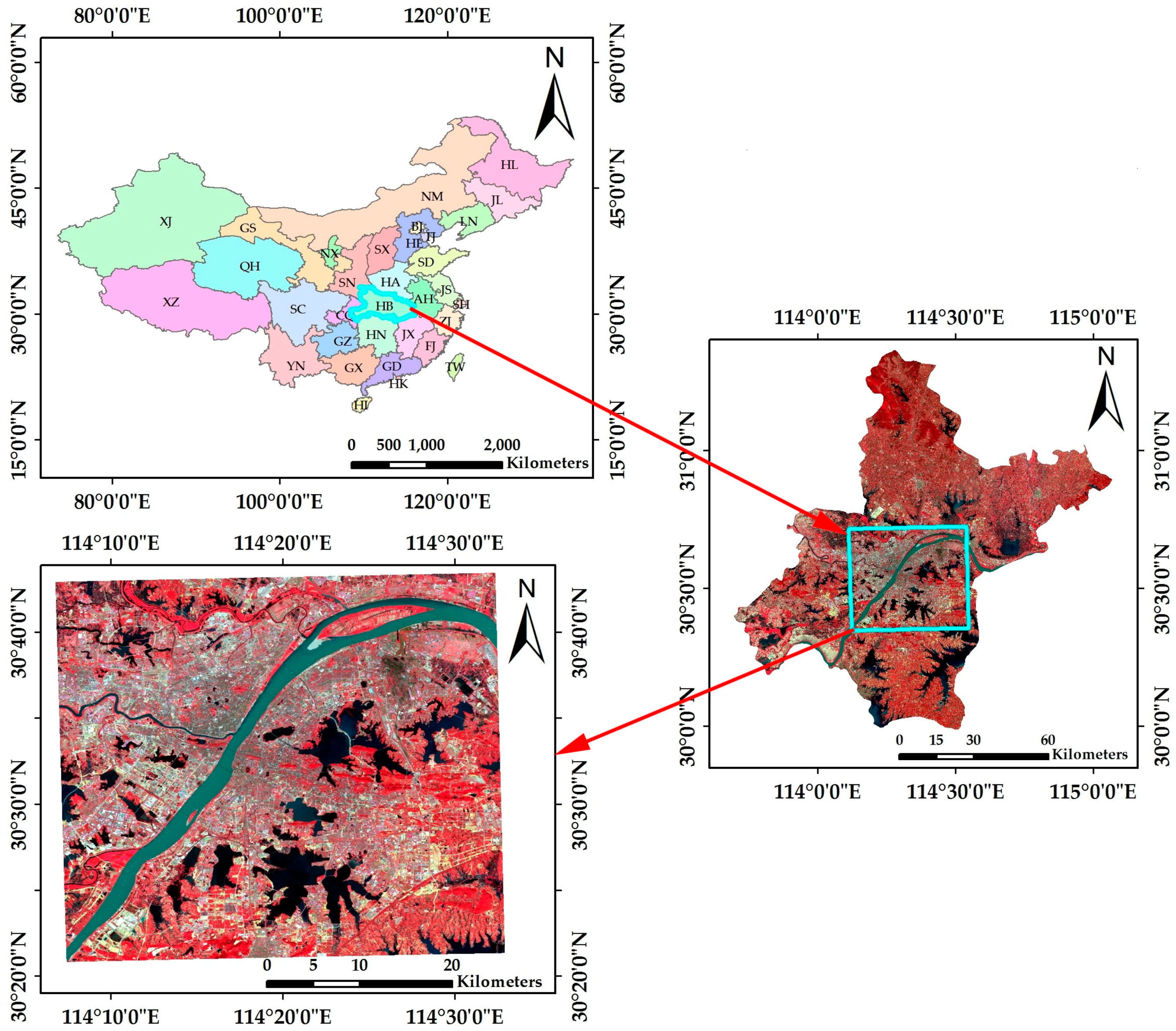
2.1. The Study Area

The study area covers the metropolitan region of Wuhan in the eastern Jianghan Plain (Figure 1). It has a tropical monsoon (humid) climate with abundant rainfall and four distinctive seasons. The annual mean temperature is 15.8 °C∼17.5 °C and the annual mean precipitation is approximately 1150 mm∼1450 mm. In the summer, the maximum air temperature in Wuhan can reach as high as 42 °C due to the terrain conditions (low and flat in the middle and hilly in the south) with the Yangtze and Han Rivers winding through the city. The main land cover types in the study area are vegetation, water bodies, bare lands, roads, residential areas and crops.

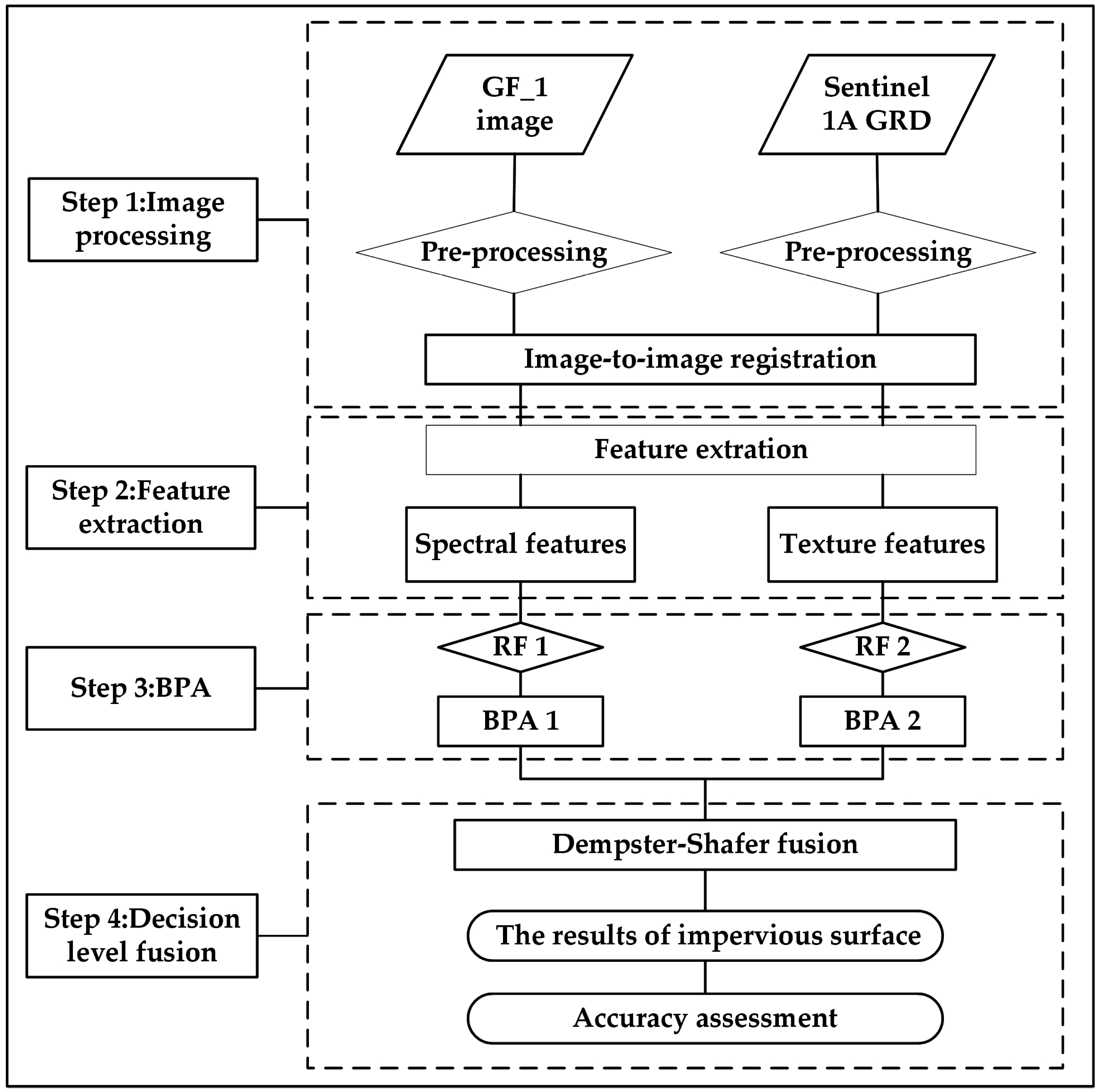
2.2. Data Sources and Preprocessing

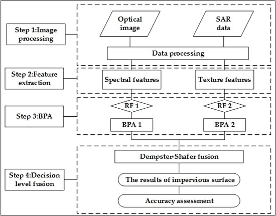
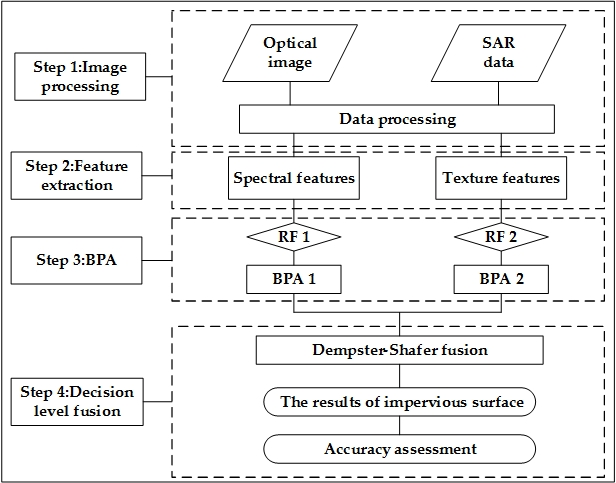
Both the GF-1 multispectral and the Sentinel-1A data were used in the study. Two GF-1 images with the spatial resolution of 16 m, acquired on 14 April 2015, were downloaded from the geospatial data cloud [47]. The images were mosaicked and subset to the study area. The images were atmospherically calibrated to the surface reflectance using the FLAASH atmospheric correction module and geometrically corrected (the RPC Orthorectification workflow) using the 30 m DEM within the ENVI 5.2 software (Exelis Visual Information Solutions, Boulder, CO, USA).

The corresponding Sentinel-1A images acquired on 17 February 2015 were downloaded from the Sentinels Scientific Data Hub [48]. Both images were HH (horizontal transmit and horizontal receive) and HV (horizontal transmit and vertical receive) polarized in the IW (interferometric wide swath) mode and were generated in the high-resolution Level-1 ground range detected (GRD) format. The high-resolution GRD product has the ground range and azimuth resolution of 5 m and 20 m, respectively. Some standard SAR preprocessing procedures, including slice assembly, radiometric calibration, multi-look, and terrain correction, were applied to the Sentinel-1A data using the SNAP software (Sentinel Application Platform, funded by ESA’s (European Space Agency) Scientific Exploitation of Operational Missions (SEOM), developed by Brockmann Consult, Array Systems Computing and C-S). The resulting mean ground pixel size was 10.00 m.

Both optical and SAR images were co-registered to the same reference system of universal transverse Mercator (UTM) projection (Zone 48N) with the datum of world geodetic system 84 (WGS84). A total of 21 control points were manually selected and the linear transformation was used to co-register the GF-1 and Sentinel-1A data. The co-registered optical and SAR data have the spatial resolution of 16 m. The root mean square error (RMSE) for the co-registration is less than half a pixel (8 m).

3. Methodology

This study fused optical and SAR data at the decision level to estimate urban impervious surface based on the random forest (RF) classifier and the evidence theory, and then analyzed the uncertainty levels for the impervious surfaces. Four steps were performed in this section in order to integrate optical and SAR data at the decision level. In the first step, both optical and SAR images were preprocessed to the same spatial resolution within the same projection system. In the second step, spectral and texture features were extracted from the GF-1 and Sentinel-1A images, respectively. Then impervious surfaces were estimated from four different data sources with the aid of the RF classifier. Finally, the impervious surfaces characterized by different datasets were fused based on the D-S theory. Figure 2 presents the overall workflow of the data-fusion procedures:

Step 1: Image processing: This step is outlined in Section 2.2.

Step 2: Feature extraction (Section 3.1): The spectral features from GF-1 image, NDVI (normalized difference vegetation index, NDVI), NDWI (normalized difference water index, NDWI) were extracted and the texture features from Sentinel-1A data were obtained.

Step 3: The RF classification (Section 3.2): Four data sources, i.e., the GF-1 image, Sentinel-1A image, GF-1 image and its spectral features (Section 3.1), and Sentinel-1A image and its texture features (Section 3.1) were used independently to quantify urban impervious surfaces which were regarded as evidence sources.

Step 4: The construction of the BPA (basic probability assignment) function and the decision fusion: The BPA function was constructed by calculating the probability of each pixel that belongs to each category and probability of correct classification based on the RF classification. Then the RF classified impervious surfaces from the GF-1 and Sentinel-1A imagery were combined by the decision rules and then the overall confidence level was provided by using the MATLAB 2014b (MATLAB and Statistics Toolbox Release 2014b, The MathWorks, Inc., Natick, MA, USA).

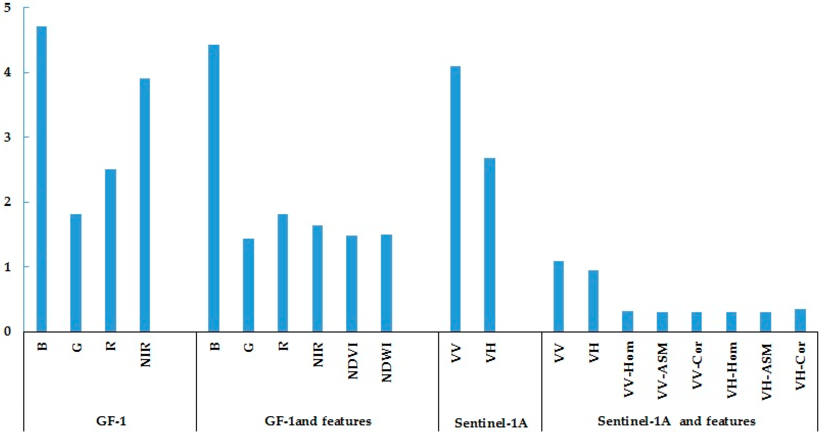
3.1. Feature Extraction

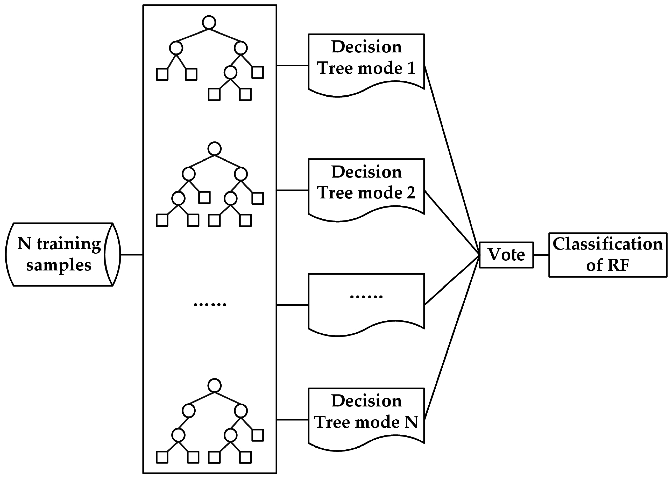
The texture feature is a set of metrics designed to quantify the perceived spatial arrangement of color or intensities. It plays a very important role in interpreting SAR data for land cover classifications. In this paper, the gray-level co-occurrence texture (GLCM) method was employed to extract texture features from the Sentinel-1A data. Haralick et al. [49] defined 14 texture statistics derived from the GLCM, i.e., the mean, correlation (Cor), variance (Var), homogeneity (Hom), contrast (Con), dissimilarity (Diss), entropy (Ent), and angular second moment (ASM) (

Table 1. The gray-level co-occurrence texture (GLCM) texture features.

Texture	Equations	Description
Mean	${\mu }_i={\displaystyle {\displaystyle \sum }_{i,j=0}^{N-1}}(P_{ij})i$ ${\mu }_j={\displaystyle {\displaystyle \sum }_{i,j=0}^{N-1}}(P_{ij})j$	Mean is the average value in the local window [50].
Correlation	${\displaystyle {\displaystyle \sum }_{i,j=0}^{N-1}}\left[\frac{\left(i-{\mu }_i\right)\left(j-{\mu }_j\right)}{\sqrt{\left({\sigma }_i^2\right)\left({\sigma }_j^2\right)}}\right]$	Correlation measures the gray level linear dependencies in the image. ${\sigma }_i^2$, ${\sigma }_j^2$ are the variance values in the local window [50,51].
Variance	${\sigma }_i^2={\displaystyle {\displaystyle \sum }_{i,j=0}^{N-1}}(P_{ij}){\left(i-{\mu }_i\right)}^2$ ${\sigma }_j^2={\displaystyle {\displaystyle \sum }_{i,j=0}^{N-1}}(P_{ij}){\left(i-{\mu }_j\right)}^2$	It is the variance in the local window [51,52].
Homogeneity	${\displaystyle {\displaystyle \sum }_{i,j=0}^{N-1}}\frac{P_{ij}}{1+{\left(i-j\right)}^2}$	Homogeneity is the smoothness of the image texture [50,51].
Contrast	${\displaystyle {\displaystyle \sum }_{i,j=0}^{N-1}}{P}_{ij}{\left(i-j\right)}^2$	Contrast measures the variations in the GLCM [50,51].
Dissimilarity	${\displaystyle {\displaystyle \sum }_{i,j=0}^{N-1}}{P}_{ij}\left|i-j\right|$	Dissimilarity is similar to the contrast measurement [50,51].
Entropy	${\displaystyle {\displaystyle \sum }_{i,j=0}^{N-1}}{P}_{ij}\left(-ln{P}_{ij}\right)$	Entropy is a measure of the degree of disorderliness in an image [50,52].
Angular Second Moment	${\displaystyle {\displaystyle \sum }_{i,j=0}^{N-1}}{P_{ij}}^2$	ASM is a measure of textural uniformity [50,52].

Note: i refers to the column number and j to the row number. $P_{ij}$ is the value in the cell i, j in the matrix. N is the number of rows or columns and equals to the number of gray levels. The pixels in the local window are indexed from zero.

). Here the study computed the texture variables using a window size of $9\times 9$ and employed all these variables for the land cover classification.

The spectral features, including NDVI and NDWI, were derived from the GF-1 image. The former index is an indicator for vegetation growth status and vegetation cover, and the latter one usually for the extraction of water areas. The two indices were expressed as below:

$$\mathrm{NDVI}=\left(\mathrm{NIR}-\mathrm{R}\right)/\left(\mathrm{NIR}+\mathrm{R}\right)$$

(1)

$$\mathrm{NDWI}=\left(\mathrm{G}-\mathrm{NIR}\right)/\left(\mathrm{G}+\mathrm{NIR}\right)$$

(2)

where R, G, and NIR refers to the surface reflectance in the red, green, and near-infrared bands, respectively.

3.2. Random Forest

Random forest was originally proposed based on the decision tree classification model by Bireman [53,54,55]. It is well suited for classification of multi-source remote sensing data by fitting a predefined number of classification trees. First, N samples are randomly selected from the original training dataset by replacement. Then classification is performed by establishing k decision trees (specified by the user) on the selected N samples. Since each decision tree provides a classification (or vote for a class), the final output of the classifier is determined by the majority vote of the decision trees [53,54,55]. Figure 3 presents the flowchart of the RF algorithm. It has been widely used in remotely sensed image classification due to the following aspects:

• The RF does not over-fit to the training set.
• Compared to other classification algorithms, the RF can deal with the noise in the dataset.
• The RF can handle data of high dimensions and does not require the feature selection. It can process the discrete data as well as the continuous data and non-standardized datasets.

In this study, two-thirds of the training samples were used to train the RF classifier and the remaining samples to evaluate the classification accuracy, known as the out-of-bag (OOB) error. The number of decision trees (Ntree) were set at the default value of 500 and the feature importance score were automatically calculated and was used to evaluate the contribution of each feature to the classification results (Figure 4). Then the land cover types were extracted individually using the RF algorithm from four data sources, including the GF-1 image, Sentinel-1A, GF-1 image and its spectral features, and Sentinel-1A image and its texture features.

3.3. The Dempster–Shafer (D-S) Theory

The fusion of urban impervious surfaces from different datasets was performed at the decision level based on the D-S theory [40,41]. The Dempster-Shafer (D-S) evidence theory is introduced by Dempster and then perfected by Shafer, which is a mathematical framework in which non-additive probability models enable us to model imprecision in beliefs. The evidence theory treats impervious surfaces estimated from different data sources as independent evidence and introduces uncertainty estimations in characterizing impervious surfaces.

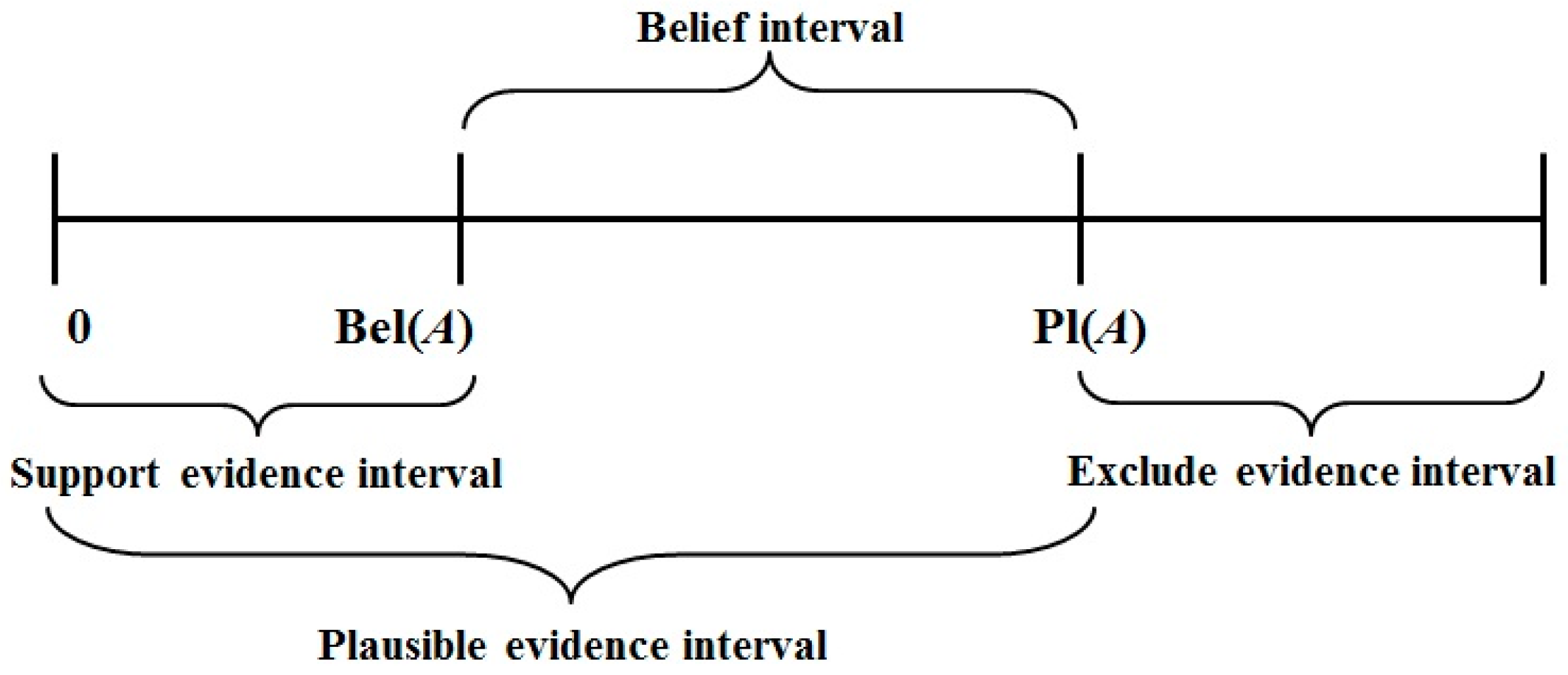
3.3.1. The Construction of the Basic Probability Assignment (BPA) and Uncertainty Interval

In this section, the procedures for the construction of the BPA function (also known as the mass function) and the calculation of the uncertainty level are described. The construction of the BPA function is a prerequisite for the fusion of impervious surfaces from different datasets at the decision level. Let Θ be the fixed set of mutually exclusive elements (also called as the frame of discernment or the hypothesis space). In this study, Θ corresponds to the land cover types including high and low albedo impervious surfaces (IS_H/IS_L), water (W), vegetation (VE), high and low reflectance of bare land (BL_H/BL_L). Θ = {IS_H, IS_L, W, VE, BL_H, and BL_L} (Figure 5).

The BPA function has to fulfill Conditions (3) and the Conditions (4)

$$\mathrm{m}(\varnothing )=0$$

(3)

$$\mathrm{and}\mathrm{m}:2^{\mathsf{\Theta }}\to \left[0,1\right]$$

$${\sum }_{\mathrm{A}\subseteq 2^{\mathsf{\Theta }}}\mathrm{m}\left(\mathrm{A}\right)=1$$

(4)

where $\varnothing$ is the empty set meaning a null proposition, A is described as a focal element of all the land cover types when m(A) > 0, and m(A) represents the degree of support for the land cover type A. In Condition (4), the value for the degree of support ranges from 0 to 1 and must sum to 1 over all possible land cover types from the hypothesis space $\mathsf{\Theta }$ = {IS_H, IS_L, W, VE, BL_H, and BL_L}.

For optical or SAR data, the evidential probability for each class can be calculated by the RF classification and assigned to each pixel. Then the BPA function is constructed using the two parameters.

$$m_i\left(A\right)=p_v*p_i$$

(5)

where $p_v$ is the vote probability of each land cover type for each pixel, and $p_i$ is the probability of correct classification.

The belief function Bel (Equation (6)) and the plausibility function Pl (Equation (7)) were defined to express the lower and upper probability (the uncertainty level interval) for a specified land cover type (Figure 6).

$$\mathrm{Bel}:2^{\mathsf{\Theta }}\to \left[0,1\right]$$

$$\mathrm{Bel}\left(\mathrm{A}\right)={\sum }_{A_i\le A}M\left(A_i\right)$$

(6)

$$\mathrm{Pl}:2^{\mathsf{\Theta }}\to \left[0,1\right]$$

$$\mathrm{Pl}\left(\mathrm{A}\right)=1-\mathrm{Bel}\left(-A_i\right)$$

(7)

They have the following properties:

$$\mathrm{Bel}\left(\mathrm{A}\right)\le \mathrm{Pl}\left(\mathrm{A}\right)$$

$$\mathrm{Pl}\left(\mathrm{A}\right)=1-Bel\left(\overline{A}\right)$$

(8)

where $\overline{A}$ is complementary to A: $\mathrm{A}\cup \overline{A}=\mathsf{\Theta }$ and $\mathrm{A}\cap \overline{A}=\varnothing$.

3.3.2. Dempster’s Combinational Rule

After calculating the BPA function (mass function) for each class, the two datasets (impervious surfaces identified individually from optical and SAR data) were converted to evidence and then were fused according to Dempster’s combinational rules. If ∀A⊆Θ, m₁ and m₂ are the mass functions in Θ, then Dempster’s combination is calculated from the two sets of masses m₁ and m₂ in the following manner:

$$\mathrm{m}(\varnothing )=0,\mathrm{A}=\varnothing$$

(9)

$$\mathrm{m}\left(\mathrm{A}\right)=m_1\oplus m_2=K^{-1}{\sum }_{A_1\bigcap A_2=A}{m}_1\left(A_1\right)m_2\left(A_2\right),A\ne \varnothing$$

(10)

$$\mathrm{K}=1-{\sum }_{A_1\bigcap A_2=\mathsf{\Phi }}{m}_1\left(A_1\right)m_2\left(A_2\right)={\sum }_{A_1\bigcap A_2\ne \mathsf{\Phi }}{m}_1\left(A_1\right)m_2\left(A_2\right)$$

(11)

where K $\in \left[0,1\right]$ is a measure of the amount of conflict between the two mass sets, a large value of K means large conflicts among different data sources and results in poor classification results by combining those data sources. The maximum value of the Bel function is used to determine the class (C_i) that a pixel belongs to. The criterion is described as the following expression:

$${\mathrm{C}}_i=\max \left(\mathrm{Bel}\left({\mathrm{A}}_i\right)\right)$$

(12)

Table 2. The mass function values of the six classes and the combination results.

Source		IS_H	IS_L	W	VE	BL_H	BL_L	M(Θ)
	Classes
Optical (m1($A_i$))		0	0	0.91	0	0	0	0.09
SAR (m2($A_i$))		0.02	0	0.29	0.02	0.03	0.42	0.22
m1(A1) $\oplus$ m2(A2)		0	0	0.89	0	0	0.07	0.04
Combination Results		A $\in$ W

Note: IS_H/IS_L—high and low albedo impervious surfaces, W—Water, VE—vegetation, BL_H/BL_L—high and low reflectance of bare land. Values for the six land cover types represents the probability that a pixel was classified to a land cover type. M (Θ) represents the uncertainty value for the land cover type identified by the specific data source. Values in this table were derived from a pixel that is located from the very bottom-right corner of the image.

shows the mass function values of the six land cover types for a pixel that was classified as low reflectance of bare land (BL_L) by using the SAR data. In Table 2, the value represented the probability that a pixel was classified as a land cover type. For example, the probability that the pixel was classified as W by using optical data was 0.91 with an uncertainty level of 0.09 (as indicated by the M (Θ)), and the probability that the pixel was classified as W by using SAR data was only 0.29 with an uncertainty level of 0.22. After the fusion procedures, the probability that this pixel would be classified as W was 0.89 but with an uncertainty level of 0.04.

3.4. Accuracy Assessment

Training and validation samples were selected by visual interpretation of the high spatial resolution Google Earth images (acquired 21 January 2015). The training samples were selected randomly among the six land covers and distributed evenly over the study area. A total of 816 pixels were finally selected as training samples, i.e., 159 points from IS_H, 180 pixels from IS_L, 113 pixels from W, 110 pixels from VE, 132 points from BL_H, and 122 pixels from BL_L. Moreover, 407 pixels were selected as validation samples, i.e., 80 pixels from IS_H, 86 pixels from IS_L, 55 pixels from W, 56 pixels from VE, 67 pixels from BL_H, and 63 pixels from BL_L. In addition to the OOB error built into the RF algorithm, the classification accuracy was also assessed by using the producer’s accuracy (PA), the user’s accuracy (UA), the overall accuracy (OA) and the Kappa coefficient based on the confusion matrix.

The confusion matrix is calculated by comparing land covers derived from the image against ground truth land cover data. Each column of the confusion matrix represents a ground truth class, and the values in the column correspond to the image’s labeling of the ground truth pixels.

The Kappa coefficient, a statistical measure of inter-rater reliability, is calculated as follows:

$$\mathrm{K}=\frac{N·{\sum }_i^r{x}_{ii}-\sum \left(x_{i+}·x_{+i}\right)}{N^2-\sum \left(x_{i+}·x_{+i}\right)}$$

(13)

where $r$ is the number of rows in the matrix, $x_{ii}$ is the number of observations in row $i$ and column $i$, $x_{i+}$ and $x_{+i}$ are the marginal totals of the row $i$ and column $i$, respectively, and N is the total number of observations.

Producer’s accuracy (PA) is the probability that a pixel is correctly classified to a land cover type, representing the errors of omission.

User’s accuracy (UA) is the proportion of pixels that are correctly classified within the image, representing the errors of commission. The overall accuracy is calculated as the ratio between the number of correctly classified pixels and the total number of pixels used for accuracy assessment.

4. Results

4.1. Land Cover Classification from the GF-1/Sentinel-1A Image/DS-Fusion

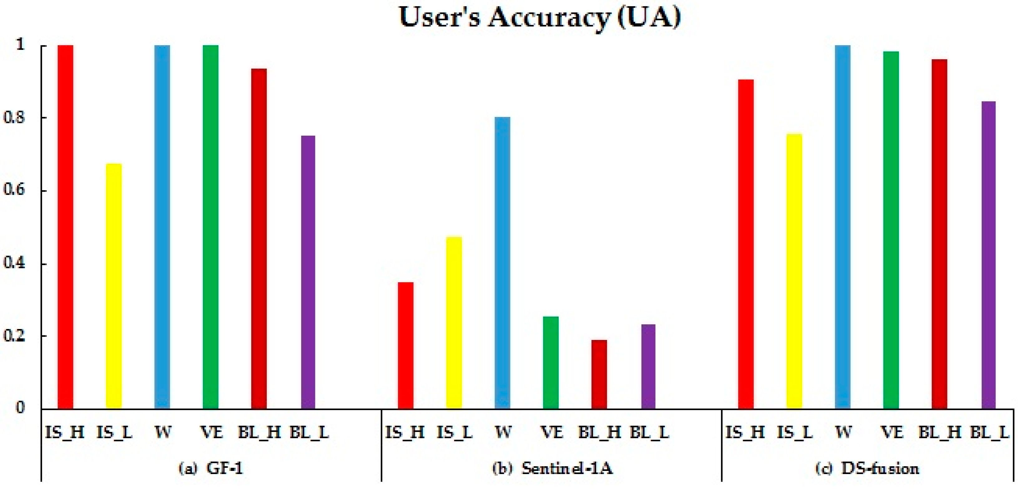
4.1.1. Land Cover Classification from the GF-1/Sentinel-1A Image

Table 3. The confusion matrix and accuracy assessment for land cover classification by using the GF-1 image/Sentinel-1A image/fusing the GF-1 and Sentinel-1A image.

Classes	IS_H	IS_L	W	VE	BL_H	BL_L
(a) GF-1
IS_H	67	0	0	0	0	0
IS_L	9	75	6	0	4	17
W	0	0	49	0	0	0
VE	0	0	0	56	0	0
BL_H	4	0	0	0	59	0
BL_L	0	11	0	0	4	46
	OA	86.49%	KAPPA	0.84
(b) Sentinel-1A
IS_H	23	9	3	7	12	12
IS_L	23	42	0	7	15	2
W	3	1	41	1	1	4
VE	14	15	1	16	7	10
BL_H	9	12	8	8	13	19
BL_L	8	7	2	17	19	16
	OA	37.10%	KAPPA	0.24
(c) DS-fusion
IS_H	70	2	0	0	3	3
IS_L	7	81	0	0	5	10
W	0	0	55	0	0	0
VE	1	0	0	56	0	0
BL_H	2	0	0	0	54	0
BL_L	0	3	0	0	5	50
	OA	89.93%	KAPPA	0.88

a shows the accuracy assessment for land cover types identified from the GF-1 image. The producer’s accuracies were 83.75%, 89.09%, and 100% (Figure 7a) and the user’s accuracies of IS_H, W, and VE were all 100% (Figure 8a), respectively. The classification of BL_H also yielded high producer’s and user’s accuracies. However, confusions were mainly observed between IS_L and BL_L and W (Table 3a), indicating the difficulty of optical data in separating land covers of similar spectral signatures. The overall accuracy of 86.49% with a Kappa coefficient of 0.84 suggested that urban impervious surfaces extracted from the GF-1 image were acceptable.

Table 3b shows the accuracy assessment for land covers identified from the Sentinel-1A image. Both the producer’s and user’s accuracies were significantly reduced by using SAR instead of optical data (Figure 7a,b and Figure 8a,b). The omission and commission errors increased dramatically for land cover types of IS_H and IS_L identified from the Sentinel-1A image than from the GF-1 image. The user’s accuracies of the IS_H and IS_L were only 34.85% and 47.19%, respectively, while the producer’s accuracies were only 28.75% and 48.84%, respectively (Figure 7b and Figure 8b). In addition, classification accuracies of vegetation and bare soils were extremely low when using the Sentinel-1A imagery. However, it should be noted that SAR data was successful in classifying water. The overall classification accuracy and Kappa coefficient were 37.10% and 0.24, respectively.

4.1.2. Fusion of Land Covers Derived from the GF-1 Image and the Sentinel-1A Image

The fused land cover types were finally generated by combining the land cover types classified independently by the GF-1 image and the Sentinel-1A image according to the D-S combination rules. Table 3c shows the confusion matrix and accuracy assessment for the land cover classification. After the decision-level fusion, the user’s accuracy of IS_H and VE were 89.74% and 98.25% and the producer’s accuracies of IS_H and VE were 87.50% and 1. The producer’s and user’s accuracies of W in Table 3c remain the same as in Table 3a. The integration of SAR data with optical data increased the user’s accuracy of BL_H to 96.43% while reducing the producer’s accuracy to 80.60% (Figure 7a,c and Figure 8a,c). Compared to the classification result by using optical data, the fused classification result reduced the commission errors from 32.40% to 21.36% for IS_L and from 24.60% to 13.79% for BL_L while decreasing the omission errors from 12.80% to 5.81% for IS_L and from 26.98% to 20.60% for BL_L (Figure 7a,c and Figure 8a,c). Clearly, Table 3c shows that the fusion of optical and SAR data reduced confusion between dark impervious surfaces and water and bare soils. The overall classification accuracy and the Kappa coefficient after the D-S fusion reached 89.93% and 0.88, respectively, higher than the 86.49% and 0.836 achieved by using the GF-1 data (Table 3a,c).

4.2. Land Cover Classification from the GF-1 Image/Sentinel-1A Image with Features/D-S Fusion

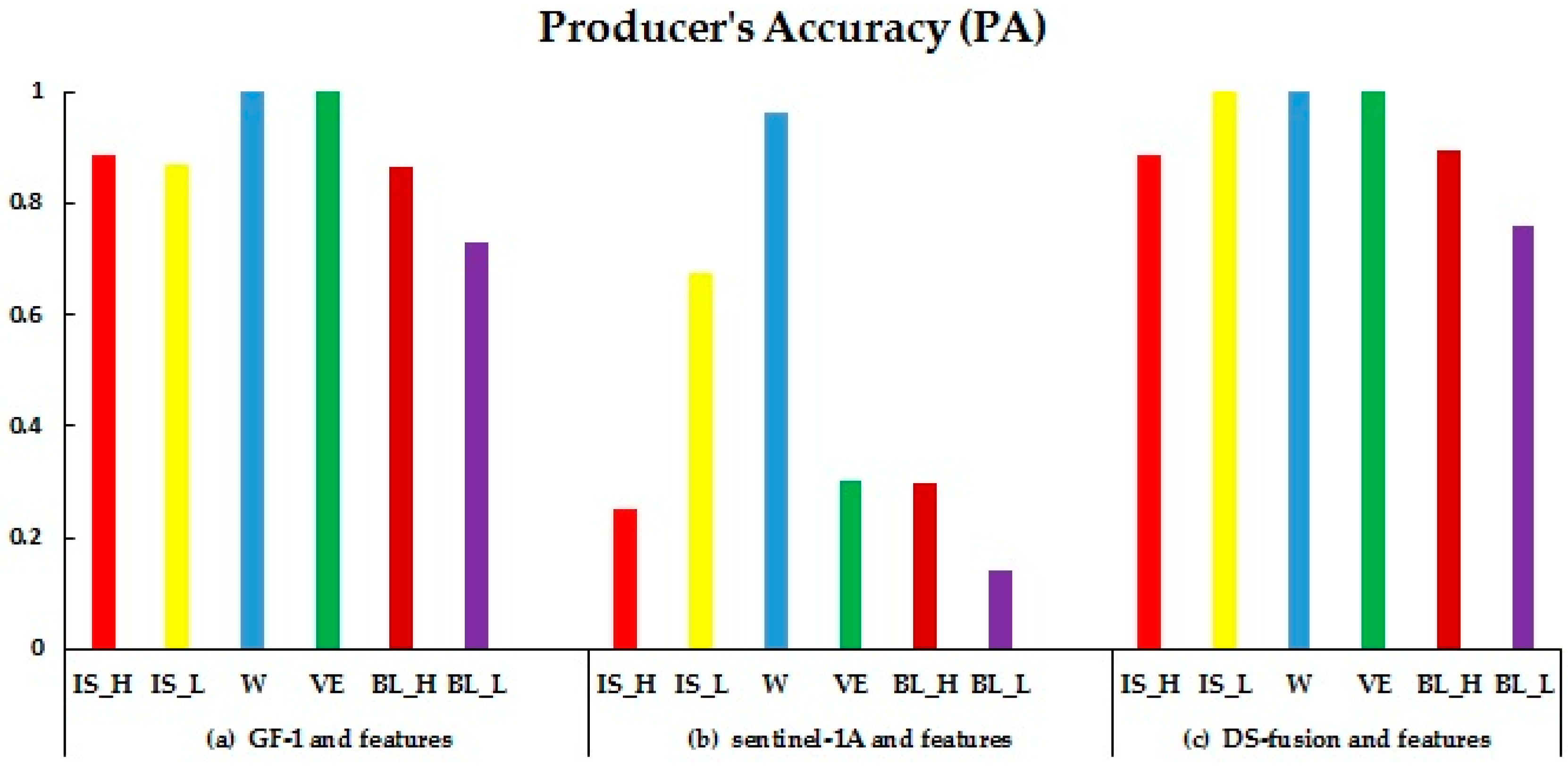
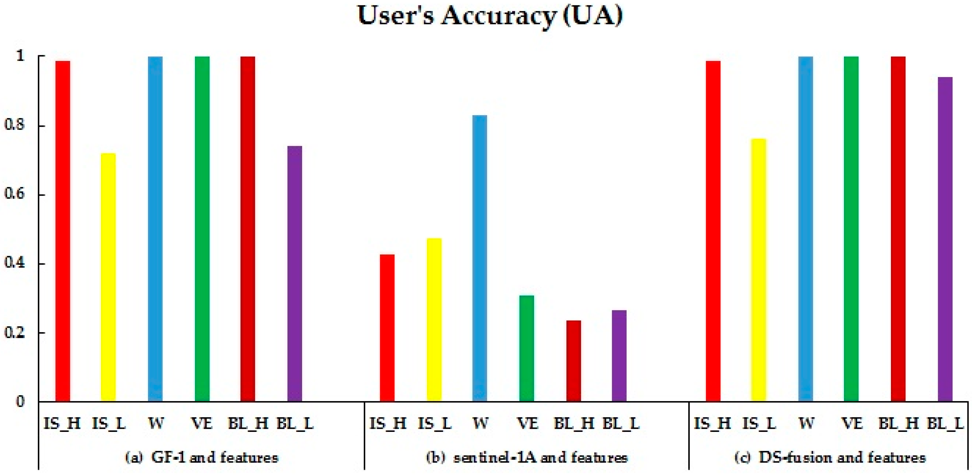
4.2.1. Land Cover Classification from the GF-1 Image/Sentinel-1A Image with Features

In this case, the spectral features NDVI and NDWI derived from the GF-1 image were used to characterize urban impervious surfaces.

Table 4. The confusion matrix and accuracy assessment for land cover classification by using the GF-1 image and its spectral features/the Sentinel-1A image and its texture features/fusing the GF-1 and Sentinel-1A images and their features.

Classes	IS_H	IS_L	W	VE	BL_H	BL_L
(a) GF-1 and features
IS_H	71	0	0	0	0	1
IS_L	9	75	0	0	4	16
W	0	0	55	0	0	0
VE	0	0	0	56	0	0
BL_H	0	0	0	0	58	0
BL_L	0	11	0	0	5	46
	OA	88.70%	KAPPA	0.86
(b) Sentinel-1A and features
IS_H	20	4	2	4	9	8
IS_L	34	58	0	10	19	1
W	6	0	53	0	0	5
VE	9	15	0	17	6	8
BL_H	7	9	0	17	20	32
BL_L	4	0	0	8	13	9
	OA	43.49%	KAPPA	0.32
(c) DS-fusion and features
IS_H	71	0	0	0	0	1
IS_L	9	86	0	0	4	14
W	0	0	55	0	0	0
VE	0	0	0	56	0	0
BL_H	0	0	0	0	60	0
BL_L	0	0	0	0	3	48
	OA	92.38%	KAPPA	0.91

a shows the confusion matrix and accuracy assessment for the six land covers. Compared with the single GF-1 image, the addition of spectral features improved the user’s accuracies from 67.60% to 72.12% for IS_L, from 93.65% to 100% for BL_H, but decreased from 100% to 98.61% for IS_H, from 75.40% to 74.19% for BL_L. The producer’s accuracies increased from 83.75% to 88.75% for IS_H, from 89.09% to 100% for W, and reduced from 88.06% to 86.60% for BL_H (Figure 7a, Figure 8a, Figure 9a and Figure 10a). The combined use of spectral features and the original image reduced confusions between IS_H and BL_H, IS_L and W. It was observed that W and VE can be fully identified with the help of NDWI and NDVI (Table 4a). The overall classification accuracy and the Kappa coefficient were 88.70% and 0.86, respectively.

In addition to the Sentinel-1A image, additional texture features were calculated from the HH and HV bands and then used for mapping urban impervious surfaces. Table 4b shows that the incorporation of texture features enhanced the classification accuracy for the six land cover types compared with using the Sentinel-1A imagery only (Table 3b). The confusion between IS_L and W was significantly reduced when adding texture features into the original Sentinel-1A data (Table 4b). However, the overall classification accuracy (43.49%) in this case is still lower than that based on the GF-1 image (86.49%).

4.2.2. Fusion of Land Covers Derived from the GF-1 and Sentinel-1A Images with Features

The land cover types derived from the integration of the GF-1 image and its spectral features and the Sentinel-1 A image and its texture feature had higher producer’s and user’s accuracies compared to those characterized independently by the GF-1 image and its spectral features or the Sentinel-1A image and its texture features. Compared to the fusion of the GF-1 image and the Sentinel-1A image, the integration of the GF-1 image and the Sentinel-1A image and their features decreased the user’s accuracy from 78.64% to 76.11% for IS_L and increased the producer’s accuracy from 94.19% to 100% for IS_L (Figure 7c, Figure 8c, Figure 9c and Figure 10c). In addition, the user’s accuracy increased from 89.74% to 98.61% for IS_H, from 98.25% to 100% for VE, from 96.43% to 100% for BL_H, and from 86.21% to 94.12% for BL_L. The producer’s accuracy increased from 87.50% to 88.75% for IS_H, and from 80.60% to 89.55% for BL_H, but decreased from 79.40% to 76.19% for BL_L (Figure 7c, Figure 8c, Figure 9c and Figure 10c). Table 4c also shows fewer confusions between IS_L and W compared to Table 3c. Overall, the classification accuracy of the fused land covers, when the spectral and texture features were introduced, was 92.38% with a Kappa coefficient of 0.91.

5. Discussion

5.1. The Classification Accuracy for Impervious Surfaces and Uncertainty Analysis

5.1.1. The Classification Accuracy for Impervious Surfaces

The identified six land cover types were further categorized as non-impervious surface (NIS) and impervious surface. The IS_H and IS_L were combined as the IS and the rest of land covers as the NIS. The impervious surface maps derived from different data sources were shown in Figure 11.

Table 5. The confusion matrix and accuracy assessment of IS and NIS derived from different data sources.

	GF-1		Sentinel-1A		DS-Fusion		GF-1 and Features		Sentinel-1A and Features		DS Fusion and Features
Classes	IS	NIS	IS	NIS	IS	NIS	IS	NIS	IS	NIS	IS	NIS
IS	151	27	97	58	160	21	155	21	116	53	166	19
NIS	15	214	69	183	6	220	11	220	50	188	0	222
Kappa	0.79		0.35		0.87		0.84		0.48		0.91
OA	89.68%		68.80%		93.37%		92.14%		74.70%		95.33%

shows that the overall classification accuracy of urban impervious surfaces extracted from the GF-1 image was 89.68% with a Kappa coefficient of 0.79, higher than those quantified from the Sentinel-1A image. The addition of spectral and texture features improved the classification accuracies of impervious surfaces extracted from the Sentinel-1A and GF-1 images. The combined use of the GF-1 image and its spectral features increased the overall accuracy by 2.46%, and the Kappa coefficient by 0.05 compared to using the GF-1 image only for generating impervious surfaces. The combined use of the Sentinel-1A image and its texture features improved the overall accuracy by 5.90% compared to using the Sentinel-1A image only for characterizing impervious surfaces. By incorporating the feature information, the decision-level fusion improved the overall classification accuracy to 95.33% with a Kappa coefficient of 0.91.

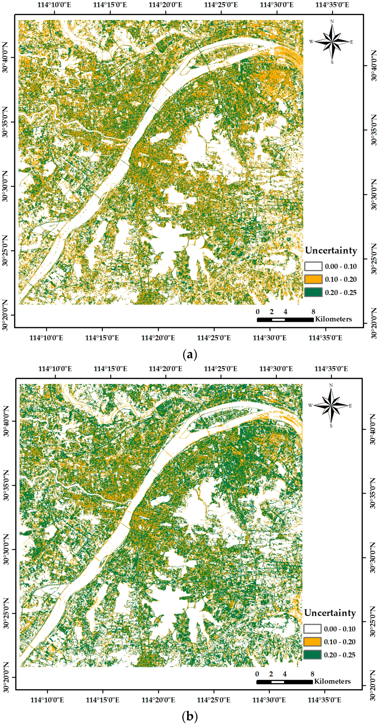
5.1.2. Uncertainty Analysis

Figure 12 shows the spatial distributions of the uncertainty values for the impervious surfaces derived by fusing the GF-1 and Sentinel-1A images (a) and by fusing the GF-1 and Sentinel-1A images and their features (b). Results indicated that the uncertainty values for the fused impervious surfaces ranged from 0 to 0.25 as shown in

Table 6. The uncertainty statistics for impervious surfaces derived by fusing the GF-1 and Sentinel-1A images/the GF-1 and Sentinel-1A images and their features.

	Minimum	Maximum	Mean	Standard Deviation
Fusing the GF-1 and Sentinel-1A images	0	0.25	0.11	0.088
Fusing the GF-1 and Sentinel-1A images and their features	0	0.25	0.11	0.093

. The land cover maps estimated by integrating the GF-1 and Sentinel-1A images as well as by the GF-1 and Sentinel-1A images and their features, had a mean uncertainty value of 0.11, though with the standard deviation of 0.088 and 0.093, respectively. We further calculated the number of pixels that fell into different uncertainty value ranges (0–0.10; 0.10–0.20; 0.20–0.25) as shown in

Table 7. The number of pixels falling into the different uncertainty value ranges for impervious surfaces derived by fusing different data sources.

Uncertainty Value Range	Fusing the GF-1 and Sentinel-1A Images	Fusing the GF-1 and Sentinel-1A Images and Their Features
	The Number of Pixels
0.00–0.10	2,888,513	2,944,986
0.10–0.20	2,546,273	2,297,449
0.20–0.25	1,098,349	1,290,700

. Nearly all water pixels were in the first range (0–0.10) (Figure 12). This could be attributed to the ability of SAR data to successfully identify the water. Overall, the fusion of the GF-1 and Sentinel-1A images with their features increased the number of pixels that fell into the first range compared to the fusion of the GF-1 and Sentinel-1A images (Table 7). It indicated that the additional feature information reduced misclassifications between IS and W. However, confusions between IS_L and BL_L still existed, thus leading to the higher number of observed pixels in the third range (0.20–0.25) for the impervious surfaces derived by integrating the GF-1 and Sentinel-1A images with their features.

5.2. Future Work

In this study, impervious surfaces were extracted by synergistically utilizing optical and SAR data based on both the RF classifier and D-S theory. Results showed that the higher classification accuracy of IS was achieved by fusing GF-1 and Sentinel-1A images and their features.

Initially, six land cover types were classified based on the RF algorithm by using GF-1/Sentinel-1A images, GF-1 image and its spectral features/Sentinel-1A image and its texture features. The accuracy assessment suggested that urban impervious surfaces extracted from the GF-1 image/GF-1 image and its spectral features were acceptable. Because of the spectral similarity, there were still confusions between IS_L and BL_L and waterbodies. Thus, spectral features NDVI and NDWI were introduced. Although the confusions between IS_L and BL_L and water were reduced, they still existed. Possible reasons could be that only two spectral features were considered in this study. Indices, such as NDISI (normalized difference impervious surface index) [19], BCI (biophysical composition index) [56], BASI (built-up areas saliency index) [57] should also be included for further improvements. In addition, the number of decision trees and the number of variables sampled at each split are the main parameters that affect the classification performance of the RF algorithm. Thus future work can be directed towards the optimization of those parameters within the RF.

Although impervious surface derived from the fused datasets had a high classification accuracy, confusions between IS_L and W and bare soils were not completely removed. Thus, the uncertainty analysis was also provided to show the reliability of the classification results. In this study, water could be easily identified with the uncertainty value less than 0.11, whereas for most of the IS pixels the uncertainty level was greater than 0.11 but less than 0.25. It is worth noting that the poor classification results from the Sentinel-1A data can significantly influence the combination results. Further refinements can be done by taking weights among different sources of evidence within the D-S framework. Finally, the effectiveness of the proposed decision-fusion level approach should be further assessed in the future by taking into consideration more case studies.

6. Conclusions

The major contribution of this study was to characterize impervious surfaces by fusing the GF-1 and Sentinel-1A data at the decision level. The advantage of the decision-level fusion was the removal of the influences of data noises and feature selections on the land cover classifications. First, four data sources, including the GF-1 image, the Sentinel-1A image, the GF-1 image and its spectral features, and the Sentinel-1A image and its texture features, were independently utilized through the random forest (RF) algorithm for characterizing impervious surfaces. Then, impervious surfaces were generated by fusing previously estimated impervious surfaces extracted individually from different data sources via the Dempster-Shafer (D-S) combination rules. The accuracy assessment illustrated that urban impervious surfaces extracted from optical data had a higher classification accuracy (89.68%) than those from synthetic aperture radar (SAR) data (68.80%). The integration of feature information with optical (or SAR data) enhanced the overall classification accuracy by 2.64% (or 5.90%). The fusion of impervious surfaces extracted from the GF-1 and the Sentinel-1A images improved the overall classification accuracy to 93.37% or to 95.33% when addition spectral and texture features were included. It was concluded that the decision-level fusion mainly reduced the confusions between the low reflectance of impervious surfaces and water and the low reflectance of the bare land.

References

1. Slonecker, E.T.; Jennings, D.B.; Garofalo, D. Remote sensing of impervious surfaces: A review. Remote Sens. Rev. 2001, 20, 227–255. [Google Scholar] [CrossRef]
2. Weng, Q. Remote sensing of impervious surfaces in the urban areas: Requirements, methods, and trends. Remote Sens. Environ. 2012, 117, 34–49. [Google Scholar] [CrossRef]
3. Arnold, C.L.; Gibbons, C.J. Impervious Surface Coverage: The Emergence of a Key Environmental Indicator. J. Am. Plan. Assoc. 1996, 62, 243–258. [Google Scholar] [CrossRef]
4. Li, J.; Song, C.; Cao, L.; Zhu, F.; Meng, X.; Wu, J. Impacts of landscape structure on surface urban heat islands: A case study of Shanghai, China. Remote Sens. Environ. 2011, 115, 3249–3263. [Google Scholar] [CrossRef]
5. Hurd, J.D.; Civco, D.L. Temporal Characterization of impervious surfaces for the State of Connecticut. In Proceedings of the ASPRS Annual Conference, Denver, CO, USA, 23–28 May 2004.
6. Yang, L.; Huang, C.; Homer, C.G.; Wylie, B.K.; Coan, M.J.; Corporation, R.; Survey, G.; Data, E.; Falls, S.; Usgs, L.Y.; et al. An approach for mapping large-area impervious surfaces: Synergistic use of Landsat 7 ETM+ and high spatial resolution imagery. Can. J. Remote Sens. 2003, 29, 230–240. [Google Scholar] [CrossRef]
7. Brabec, E.; Schulte, S.; Richards, P.L. Impervious Surfaces and Water Quality: A Review of Current Literature and Its Implications for Watershed Planning. J. Plan. Lit. 2002, 16, 499–514. [Google Scholar] [CrossRef]
8. Lu, D.; Li, G.; Kuang, W.; Moran, E. Methods to extract impervious surface areas from satellite images. Int. J. Digit. Earth 2014, 7, 93–112. [Google Scholar] [CrossRef]
9. Weng, Q.; Hu, X. Medium spatial resolution satellite imagery for estimating and mapping urban impervious surfaces using LSMA and ANN. IEEE Trans. Geosci. Remote Sens. 2008, 46, 2397–2406. [Google Scholar] [CrossRef]
10. Zhang, L.; Weng, Q. Annual dynamics of impervious surface in the Pearl River Delta, China, from 1988 to 2013, using time series Landsat imagery. ISPRS J. Photogramm. Remote Sens. 2016, 113, 86–96. [Google Scholar] [CrossRef]
11. Shao, Z.; Liu, C. The integrated use of DMSP-OLS nighttime light and MODIS data for monitoring large-scale impervious surface dynamics: A case study in the Yangtze River Delta. Remote Sens. 2014, 6, 9359–9378. [Google Scholar] [CrossRef]
12. Ridd, M.K. Exploring a V-I-S (vegetation-impervious surface-soil) model for urban ecosystem analysis through remote sensing: Comparative anatomy for cities†. Int. J. Remote Sens. 1995, 16, 2165–2185. [Google Scholar] [CrossRef]
13. Wu, C.; Murray, A.T. Estimating impervious surface distribution by spectral mixture analysis. Remote Sens. Environ. 2003, 84, 493–505. [Google Scholar] [CrossRef]
14. Lu, D.; Weng, Q. Use of impervious surface in urban land-use classification. Remote Sens. Environ. 2006, 102, 146–160. [Google Scholar] [CrossRef]
15. Deng, C.; Wu, C. The use of single-date MODIS imagery for estimating large-scale urban impervious surface fraction with spectral mixture analysis and machine learning techniques. ISPRS J. Photogramm. Remote Sens. 2013, 86, 100–110. [Google Scholar] [CrossRef]
16. Kuang, W.; Liu, J.; Zhang, Z.; Lu, D.; Xiang, B. Spatiotemporal dynamics of impervious surface areas across China during the early 21st century. Chin. Sci. Bull. 2012, 58, 1691–1701. [Google Scholar] [CrossRef]
17. Wu, C. Normalized spectral mixture analysis for monitoring urban composition using ETM+ imagery. Remote Sens. Environ. 2004, 93, 480–492. [Google Scholar] [CrossRef]
18. Deng, C.; Wu, C. A spatially adaptive spectral mixture analysis for mapping subpixel urban impervious surface distribution. Remote Sens. Environ. 2013, 133, 62–70. [Google Scholar] [CrossRef]
19. Xu, H. Analysis of Impervious Surface and its Impact on Urban Heat Environment using the Normalized Difference Impervious Surface Index (NDISI). Photogramm. Eng. Remote Sens. 2010, 76, 557–565. [Google Scholar] [CrossRef]
20. Liu, C.; Shao, Z.; Chen, M.; Luo, H. MNDISI: A multi-source composition index for impervious surface area estimation at the individual city scale. Remote Sens. Lett. 2013, 4, 803–812. [Google Scholar] [CrossRef]
21. Wang, Z.; Gang, C.; Li, X.; Chen, Y.; Li, J. Application of a normalized difference impervious index (NDII) to extract urban impervious surface features based on Landsat TM images. Int. J. Remote Sens. 2015, 36, 1055–1069. [Google Scholar] [CrossRef]
22. Chabaeva, A.; Civco, D.; Prisloe, S. Development of a population density and land use based regression model to calculate the amount of imperviousness. In Proceedings of the ASPRS Annual Conference, Denver, CO, USA, 23–28 May 2004.
23. Elvidge, C.D.; Tuttle, B.T.; Sutton, P.C.; Baugh, K.E.; Howard, A.T.; Milesi, C.; Bhaduri, B.; Nemani, R. Global Distribution and Density of Constructed Impervious Surfaces. Sensors 2007, 7, 1962–1979. [Google Scholar] [CrossRef]
24. Bauer, M.E.; Loffelholz, B.; Wilson, B. Estimating and mapping impervious surface area by regression analysis of Landsat imagery. In Remote Sensing Impervious Surface; CRC Press: Boca Raton, FL, USA, 2008. [Google Scholar]
25. Lu, D.; Tian, H.; Zhou, G.; Ge, H. Regional mapping of human settlements in southeastern China with multisensor remotely sensed data. Remote Sens. Environ. 2008, 112, 3668–3679. [Google Scholar] [CrossRef]
26. Hodgson, M.E.; Jensen, J.R.; Tullis, J.A.; Riordan, K.D.; Archer, C.M. Synergistic Use of Lidar and Color Aerial Photography for Mapping Urban Parcel Imperviousness. Photogramm. Eng. Remote Sens. 2003, 69, 973–980. [Google Scholar] [CrossRef]
27. Powell, S.L.; Cohen, W.B.; Yang, Z.; Pierce, J.D.; Alberti, M. Quantification of impervious surface in the Snohomish Water Resources Inventory Area of Western Washington from 1972–2006. Remote Sens. Environ. 2008, 112, 1895–1908. [Google Scholar] [CrossRef]
28. Wu, C. Quantifying high-resolution impervious surfaces using spectral mixture analysis. Int. J. Remote Sens. 2009, 30, 2915–2932. [Google Scholar] [CrossRef]
29. Lu, D.; Weng, Q. Extraction of urban impervious surfaces from an IKONOS image. Int. J. Remote Sens. 2009, 30, 1297–1311. [Google Scholar] [CrossRef]
30. Mohapatra, R.P.; Wu, C. Subpixel Imperviousness Estimation with IKONOS Imagery: An Artificial Neural Network Approach. Remote Sens. Impervious Surf. 2008, 2000, 21–35. [Google Scholar]
31. Zhang, X.; Xiao, P.; Feng, X. Impervious surface extraction from high-resolution satellite image using pixel- and object-based hybrid analysis. Int. J. Remote Sens. 2013, 34, 4449–4465. [Google Scholar] [CrossRef]
32. Weng, Q.; Hu, X.; Liu, H. Estimating impervious surfaces using linear spectral mixture analysis with multitemporal ASTER images. Int. J. Remote Sens. 2009, 30, 4807–4830. [Google Scholar] [CrossRef]
33. Im, J.; Lu, Z.; Rhee, J.; Quackenbush, L.J. Impervious surface quantification using a synthesis of artificial immune networks and decision/regression trees from multi-sensor data. Remote Sens. Environ. 2012, 117, 102–113. [Google Scholar] [CrossRef]
34. Jiang, L.; Liao, M.; Lin, H.; Yang, L. Synergistic use of optical and InSAR data for urban impervious surface mapping: A case study in Hong Kong. Int. J. Remote Sens. 2009, 30, 2781–2796. [Google Scholar] [CrossRef]
35. Leinenkugel, P.; Esch, T.; Kuenzer, C. Settlement detection and impervious surface estimation in the Mekong Delta using optical and SAR remote sensing data. Remote Sens. Environ. 2011, 115, 3007–3019. [Google Scholar] [CrossRef]
36. Yang, L.M.; Jiang, L.M.; Lin, H.; Liao, M.S. Quantifying Sub-pixel Urban Impervious Surface through Fusion of Optical and InSAR Imagery. Gisci. Remote Sens. 2009, 46, 161–171. [Google Scholar] [CrossRef]
37. Zhang, H.; Zhang, Y.; Lin, H. A comparison study of impervious surfaces estimation using optical and SAR remote sensing images. Int. J. Appl. Earth Obs. Geoinform. 2012, 18, 148–156. [Google Scholar] [CrossRef]
38. Zhang, Y.; Zhang, H.; Lin, H. Improving the impervious surface estimation with combined use of optical and SAR remote sensing images. Remote Sens. Environ. 2014, 141, 155–167. [Google Scholar] [CrossRef]
39. Zhang, J.; Yang, J.; Zhao, Z.; Li, H.; Zhang, Y. Block-regression based fusion of optical and SAR imagery for feature enhancement. Int. J. Remote Sens. 2010, 31, 2325–2345. [Google Scholar] [CrossRef]
40. Dempster, A.P. Upper and lower probabilities induced by multivalue mapping. Ann. Math. Stat. 1967, 38, 325–339. [Google Scholar] [CrossRef]
41. Shafer, G. A Mathematical Theory of Evidence; Princeton University Press: Princeton, NJ, USA, 1976. [Google Scholar]
42. Lein, J.K. Applying evidential reasoning methods to agricultural land cover classification. Int. J. Remote Sens. 2003, 24, 4161–4180. [Google Scholar] [CrossRef]
43. Cayuela, L.; Golicher, D.; Salas Rey, J.; Rey Benayas, J.M. Classification of a complex landscape using Dempster-Shafer theory of evidence. Int. J. Remote Sens. 2006, 27, 1951–1971. [Google Scholar] [CrossRef]
44. Chust, G.; Ducrot, D.; Pretus, J.L. Land cover discrimination potential of radar multitemporal series and optical multispectral images in a Mediterranean cultural landscape. Int. J. Remote Sens. 2004, 25, 3513–3528. [Google Scholar] [CrossRef]
45. Ran, Y.; Li, X.; Lu, L.; Li, Z. Large-scale land cover mapping with the integration of multi-source information based on teh Dempster-Shafer theory. Int. J. Geogr. Inf. Sci. 2012, 26, 169–191. [Google Scholar] [CrossRef]
46. Lu, L.; Xie, W.; Zhang, J.; Huang, G.; Li, Q.; Zhao, Z. Woodland extraction from high-resolution CASMSAR data based on dempster-shafer evidence theory fusion. Remote Sens. 2015, 7, 4068–4091. [Google Scholar] [CrossRef]
47. GF-1 Images. Geospatial Data Cloud. Available online: http://www.gscloud.cn/ (accessed on 6 October 2015).
48. Sentinel-1A Images. Sentinels Scientific Data Hub. Available online: https://scihub.copernicus.eu/ (accessed on 11 October 2015).
49. Haralick, R.M.; Shanmugam, K.; Dinstein, I. Textural features for image classification. IEEE Trans. Syst. Man Cybern. 1973, 3, 610–621. [Google Scholar] [CrossRef]
50. Ouma, Y.O.; Tateishi, R. Optimization of Second-Order Grey-Level Texture in High-Resolution Imagery for Statistical Estimation of Above-Ground Biomass. J. Environ. Inform. 2006, 8, 70–85. [Google Scholar] [CrossRef]
51. Dye, M.; Mutanga, O.; Ismail, R. Combining spectral and textural remote sensing variables using random forests: Predicting the age of Pinus patulaforests in KwaZulu-Natal, South Africa. J. Spat. Sci. J. Spat. Sci. 2012, 57, 193–211. [Google Scholar] [CrossRef]
52. Wang, H.; Zhao, Y.; Pu, R.; Zhang, Z. Mapping Robinia pseudoacacia forest health conditions by using combined spectral, spatial, and textural information extracted from IKONOS imagery and random forest classifier. Remote Sens. 2015, 7, 9020–9044. [Google Scholar] [CrossRef]
53. Breiman, L. Bagging Predictors. Mach. Learn. 1996, 24, 123–140. [Google Scholar] [CrossRef]
54. Breiman, L.E.O. Random Forests. Mach. Learn. 2001, 45, 5–32. [Google Scholar] [CrossRef]
55. Ho, T.K. The random subspace method for constructing decision forests. IEEE Trans. Pattern Anal. Mach. Intell. 1998, 20, 832–844. [Google Scholar]
56. Deng, C.; Wu, C. BCI: A biophysical composition index for remote sensing of urban environments. Remote Sens. Environ. 2012, 127, 247–259. [Google Scholar] [CrossRef]
57. Shao, Z.; Tian, Y.; Shen, X. BASI: A new index to extract built-up areas from high-resolution remote sensing images by visual attention model. Remote Sens. Lett. 2014, 5, 305–314. [Google Scholar] [CrossRef]
Figure 1. The geographic location of the study area.
Remotesensing 08 00945 g001
Figure 2. The overall workflow for extracting urban impervious surfaces by fusing optical and synthetic aperture radar (SAR) data.
Remotesensing 08 00945 g002
Figure 3. The flowchart of the random forest (RF) algorithm.
Remotesensing 08 00945 g003
Figure 4. Feature importance.
Remotesensing 08 00945 g004
Figure 5. The frame of discernment Θ = {IS_H, IS_L, W, VE, BL_H, and BL_L}.
Remotesensing 08 00945 g005
Figure 6. The uncertainty interval measured by the belief and plausibility functions.
Remotesensing 08 00945 g006
Figure 7. The producer’s accuracy of land cover types extracted from different data sources. (a) The producer’s accuracy of land cover types extracted from GF-1 image; (b) The producer’s accuracy of land cover types extracted from Sentinel-1A image; (c) The producer’s accuracy of land cover types extracted from fusing the GF-1 and Sentinel-1A image.
Remotesensing 08 00945 g007
Figure 8. The user’s accuracy of land cover types extracted from different data sources. (a) The user’s accuracy of land cover types extracted from GF-1 image; (b) The user’s accuracy of land cover types extracted from Sentinel-1A image; (c) The user’s accuracy of land cover types extracted from fusing the GF-1 and Sentinel-1A image.
Remotesensing 08 00945 g008
Figure 9. The producer’s accuracy of land cover types extracted from different data sources. (a) The producer’s accuracy of land cover types extracted from GF-1 image and features; (b) The producer’s accuracy of land cover types extracted from Sentinel-1A image and features; (c) The producer’s accuracy of land cover types extracted from fusing the GF-1 and Sentinel-1A images with features.
Remotesensing 08 00945 g009
Figure 10. The user’s accuracy of land cover types extracted from different data sources. (a) The user’s accuracy of land cover types extracted from GF-1 image and features; (b) The user’s accuracy of land cover types extracted from Sentinel-1A image and features; (c) The user’s accuracy of land cover types extracted from fusing the GF-1 and Sentinel-1A images with features.
Remotesensing 08 00945 g010
Figure 11. Impervious surface extracted from different data sources. (a) Impervious surface (IS) from the GF-1 image; (b) IS from the Sentinel-1A image; (c) IS from the combined use of GF-1 image and its spectral features; (d) IS from the combined use the Sentinel-1A and its textural features; (e) IS from the fusion of the original optical and SAR images; (f) IS from the fusion of the original optical and SAR images and their features.
Remotesensing 08 00945 g011
Figure 12. The spatial distributions of the uncertainty levels for the fused impervious surfaces. (a) The uncertainty values of impervious surfaces derived by fusing the GF-1 and Sentinel-1A images; (b) The uncertainty values of impervious surfaces derived by fusing the GF-1 and Sentinel-1A images and their features.
Remotesensing 08 00945 g012