
Deformation and Source Parameters of the 2015 Mw 6.5 Earthquake in Pishan, Western China, from Sentinel-1A and ALOS-2 Data


Abstract
:
1. Introduction

2. Geological Background
3. InSAR Observations
3.1. SAR Data Processing

| Satellite | Track | Master | Slave | Perp. B | Inc. Angle | Azi. Angle | σ † | α ǂ |
|---|---|---|---|---|---|---|---|---|
| YYYYMMDD | YYYYMMDD | m | ° | ° | mm | km | ||
| Sentinel-1A | T056A | 20150630 | 20150724 | −53 | 33.7 | −169.3 | 6.0 | 15.0 |
| T136D | 20150624 | 20150718 | 26 | 41.4 | −9.8 | 2.5 | 9.9 | |
| ALOS-2 | P160A | 20150222 | 20150726 | −245 | 36.4 | −169.7 | 6.9 | 7.9 |
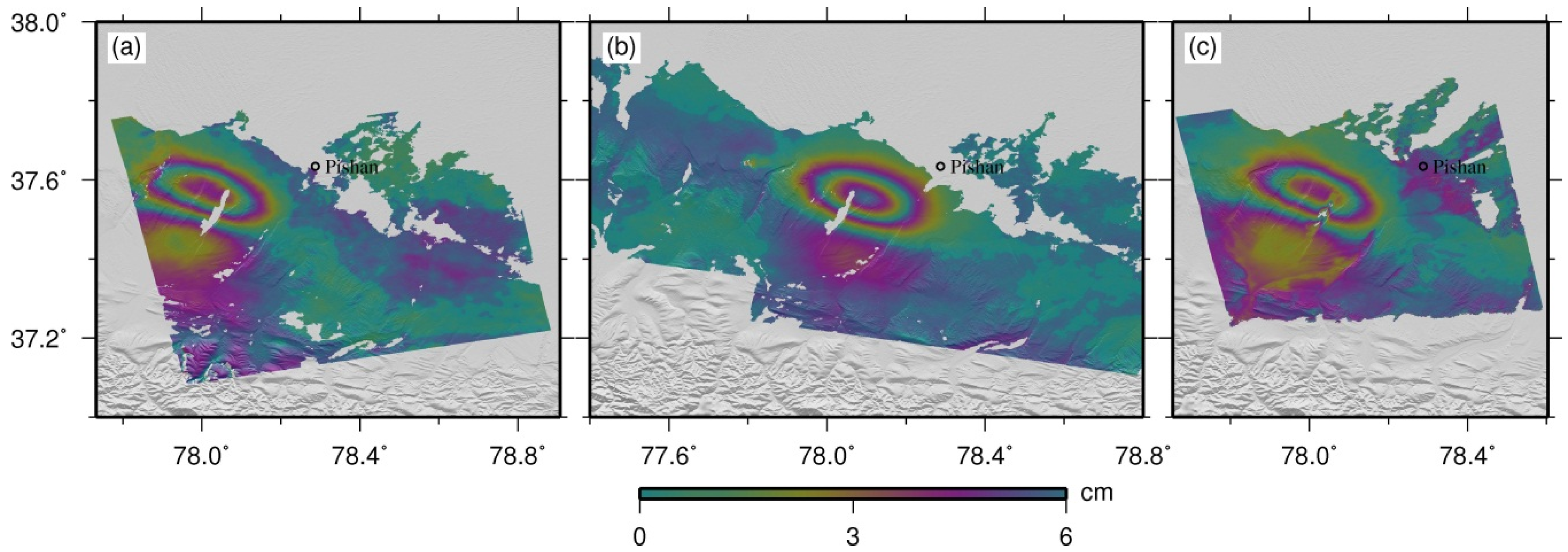
3.2. InSAR Coseismic Deformation

3.3. 2.5D Surface Deformation

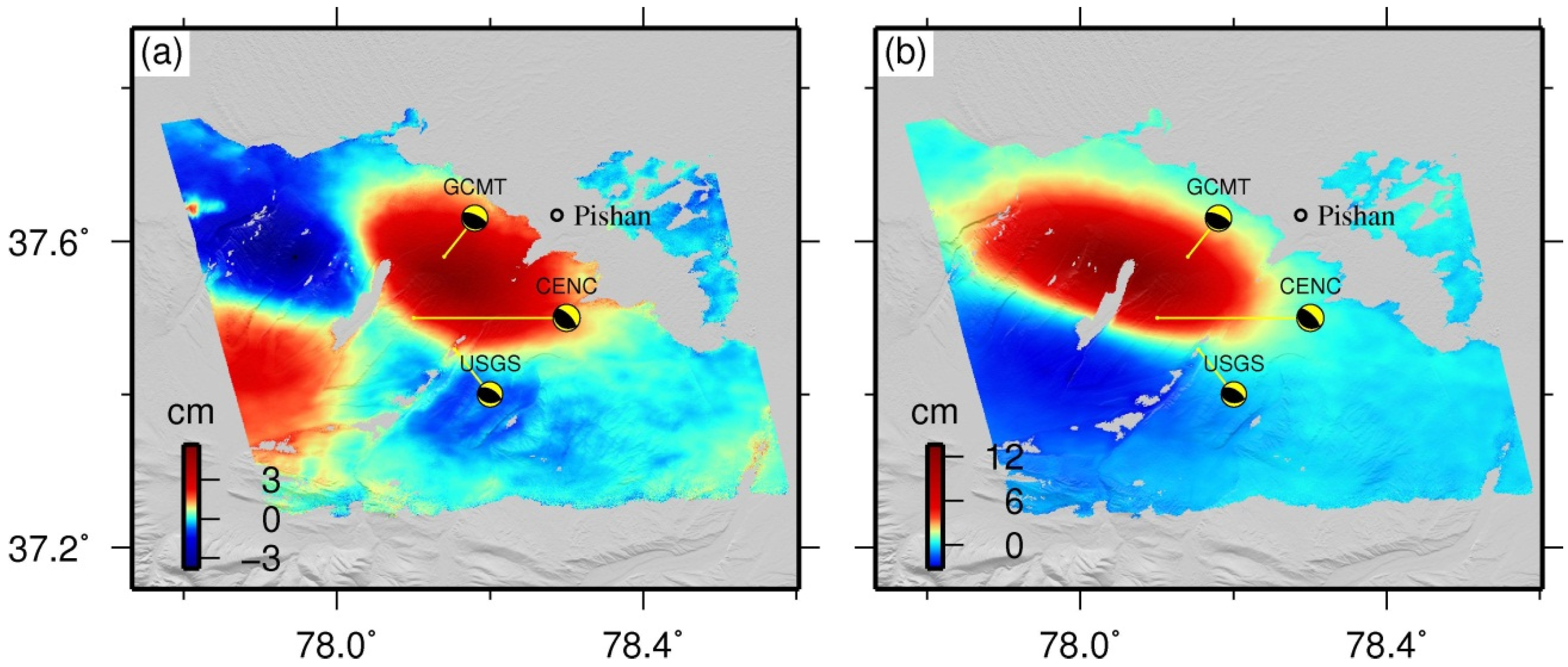
| Source | Lon. | Lat. | Strike | Dip | Rake | Depth | Length | Width | Slip | Mw |
|---|---|---|---|---|---|---|---|---|---|---|
| ° | ° | ° | ° | ° | km | km | km | m | ||
| USGS-BW | 78.154 | 37.459 | 98 | 34 | 72 | 23.0 | - | - | - | 6.2 |
| GCMT | 78.14 | 37.58 | 109 | 22 | 85 | 15.6 | - | - | - | 6.4 |
| CENC | 78.1 | 37.5 | 115 | 23 | 72 | 22 | - | - | - | 6.5 |
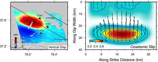
| Uniform slip model | 78.057 | 37.571 | 114.0 | 23.6 | 92.6 | 8.8 | 22.1 | 10.1 | 0.59 | 6.4 |
| ±0.4 km | ±0.3 km | ±1.6 | ±1.5 | ±3.2 | ±0.4 | ±0.5 | ±1.0 | ±0.06 | ||
| Distributed slip model | 78.057 | 37.571 | 114.0 | 25.0 | 97.0 | - | 36 | 40 | 0.34 | 6.5 |
4. Source Parameter Modeling
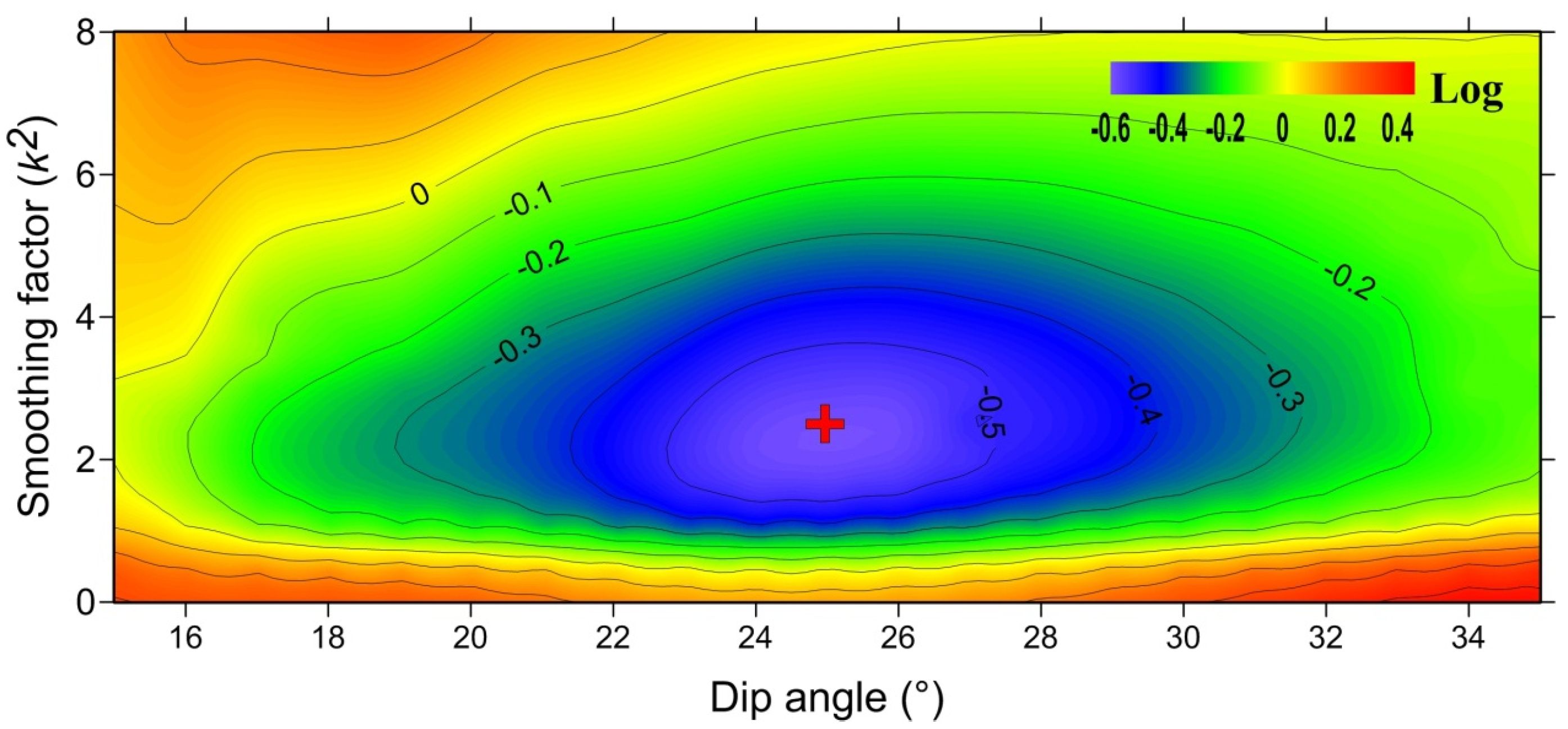
4.1. Data Reduction and Weighting
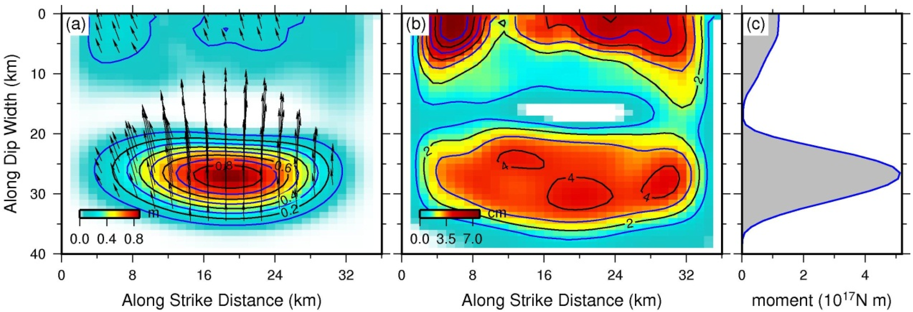
4.2. Finite Fault Slip Model


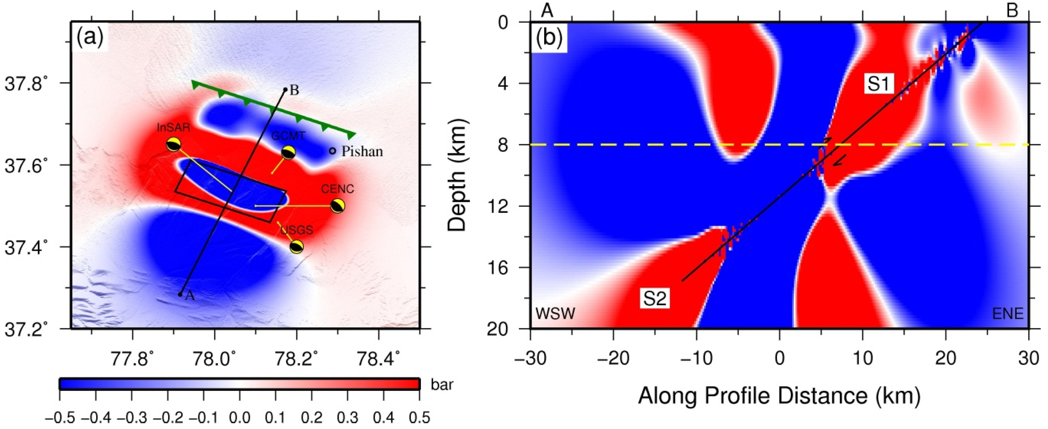
5. Stress Readjustment

6. Discussion
7. Conclusions
Acknowledgments
Author Contributions
Conflicts of Interest
References
- Lin, A.; Kano, K.-I.; Guo, J.; Maruyama, T. Late Quaternary activity and dextral strike-slip movement on the Karakax Fault Zone, northwest Tibet. Tectonophysics 2008, 453, 44–62. [Google Scholar] [CrossRef]
- Deng, Q. Map of Active Tectonics in China; Seismological Press: Beijing, China, 2007. [Google Scholar]
- Jiang, G.; Wen, Y.; Liu, Y.; Xu, X.; Fang, L.; Chen, G.; Gong, M.; Xu, C. Joint analysis of the 2014 Kangding, southwest China, earthquake sequence with seismicity relocation and InSAR inversion. Geophys. Res. Lett. 2015, 42, 3273–3281. [Google Scholar] [CrossRef]
- Walters, R.J.; Elliott, J.R.; D’Agostino, N.; England, P.C.; Hunstad, I.; Jackson, J.A.; Parsons, B.; Phillips, R.; Roberts, G. The 2009 L’Aquila Earthquake (Central Italy): An InSAR source mechanism and implications for seismic hazard. Geophys. Res. Lett. 2009, 36. [Google Scholar] [CrossRef]
- Tronin, A.A. Satellite remote sensing in seismology. A review. Remote Sens. 2010, 2, 124–150. [Google Scholar] [CrossRef]
- Jiang, G.; Xu, C.; Wen, Y.; Liu, Y.; Yin, Z.; Wang, J. Inversion for coseismic slip distribution of the 2010 Mw 6.9 Yushu Earthquake from InSAR data using angular dislocations. Geophys. J. Int. 2013, 194, 1011–1022. [Google Scholar] [CrossRef]
- Liu, Y.; Xu, C.; Wen, Y.; Fok, H.S. A new perspective on fault geometry and slip distribution of the 2009 Dachaidan Mw 6.3 earthquake from InSAR observations. Sensors 2015, 15, 16786–16803. [Google Scholar] [CrossRef] [PubMed]
- International Seismological Centre. Available online: http://www.isc.ac.uk (accessed on 23 November 2015).
- Li, J. Kinematics of Present-Day Deformation of the Tian Shan and Adjacent Regions with GPS Geodesy: Implications for Active Tectonics and Seismic Hazards. Ph.D. Thesis, China University of Geosciences, Wuhan, China, 2012. [Google Scholar]
- Ayadi, A.; Dorbath, C.; Ousadou, F.; Maouche, S.; Chikh, M.; Bounif, M.A.; Meghraoui, M. Zemmouri earthquake rupture zone (Mw 6.8, Algeria): Aftershocks sequence relocation and 3D velocity model. J. Geophys. Res. 2008, 113, 102–110. [Google Scholar] [CrossRef]
- Jiang, Z.; Wang, M.; Wang, Y.; Wu, Y.; Che, S.; Shen, Z.-K.; Burgmann, R.; Sun, J.; Yang, Y.; Liao, H.; et al. GPS constrained coseismic source and slip distribution of the 2013 Mw 6.6 Lushan, China, earthquake and its tectonic implications. Geophys. Res. Lett. 2014, 41, 407–413. [Google Scholar] [CrossRef]
- Xu, C.J.; Ding, K.H.; Cai, J.Q.; Grafarend, E.W. Methods of determining weight scaling factors for geodetic-geophysical joint inversion. J. Geodyn. 2009, 47, 39–46. [Google Scholar] [CrossRef]
- Li, S.L.; Mooney, W.D. Crustal structure of China from deep seismic sounding profiles. Tectonophysics 1998, 288, 105–113. [Google Scholar] [CrossRef]
- Molnar, P.; Tapponnier, P. Cenozoic tectonics of Asia: Effects of a continental collision. Science 1975, 189, 419–426. [Google Scholar] [CrossRef] [PubMed]
- Yin, A.; Harrison, T.M. Geologic evolution of the Himalayan-Tibetan Orogen. Annu. Rev. Earth Planet. Sci. 2000, 28, 211–280. [Google Scholar] [CrossRef]
- Avouac, J.P.; Peltzer, G. Active tectonics in southern Xinjiang, China: Analysis of terrace riser and normal fault scarp degradation along the Hotan-Qira fault system. J. Geophys. Res. 1993, 98, 21773–21807. [Google Scholar] [CrossRef]
- Matte, P.; Tapponnier, P.; Arnaud, N.; Bourjot, L.; Avouac, J.P.; Vidal, P.; Liu, Q.; Pan, Y.; Wang, Y. Tectonics of western Tibet, between the Tarim and the Indus. Earth Planet. Sci. Lett. 1996, 142, 311–330. [Google Scholar] [CrossRef]
- Shen, Z.K.; Wang, M.; Li, Y.; Jackson, D.D.; Yin, A.; Dong, D.; Fang, P. Crustal deformation along the Altyn Tagh fault system, western China, from GPS. J. Geophys. Res. 2001, 106, 30607–30621. [Google Scholar] [CrossRef]
- Peltzer, G.; Tapponnier, P.; Armijo, R. Magnitude of late Quaternary left-lateral displacements along the north edge of Tibet. Science 1989, 246, 1285–1289. [Google Scholar] [CrossRef] [PubMed]
- Wright, T.J.; Parsons, B.; England, P.C.; Fielding, E.J. InSAR observations of low slip rates on the major faults of western Tibet. Science 2004, 305, 236–239. [Google Scholar] [CrossRef] [PubMed]
- Cowgill, E.; Gold, R.D.; Xuanhua, C.; Xiao-Feng, W.; Arrowsmith, J.R.; Southon, J. Low Quaternary slip rate reconciles geodetic and geologic rates along the Altyn Tagh fault, northwestern Tibet. Geology 2009, 37, 647–650. [Google Scholar] [CrossRef]
- Yin, A.; Rumelhart, P.E.; Butler, R.; Cowgill, E.; Harrison, T.M.; Foster, D.A.; Ingersoll, R.V.; Zhang, Q.; Zhou, X.Q.; Wang, X.F.; et al. Tectonic history of the Altyn Tagh fault system in northern Tibet inferred from Cenozoic sedimentation. Geol. Soc. Am. Bull. 2002, 114, 1257–1295. [Google Scholar] [CrossRef]
- Zhou, Y.; Wang, W.M.; Xiong, L.; He, J.K. Rupture process of 12 February 2014,Yutian Mw6.9 earthquake and stress change on nearby faults. Chin. J. Geophys. 2015, 58, 184–193. [Google Scholar] [CrossRef]
- Wright, T.J.; Parsons, B.E.; Lu, Z. Toward mapping surface deformation in three dimensions using InSAR. Geophys. Res. Lett. 2004, 31, L01607. [Google Scholar] [CrossRef]
- Liu, Y.; Xu, C.; Wen, Y.; He, P.; Jiang, G. Fault rupture model of the 2008 Dangxiong (Tibet, China) Mw 6.3 earthquake from Envisat and ALOS data. Adv. Space Res. 2012, 50, 952–962. [Google Scholar] [CrossRef]
- Torres, R.; Snoeij, P.; Geudtner, D.; Bibby, D.; Davidson, M.; Attema, E.; Potin, P.; Rommen, B.; Floury, N.; Brown, M.; et al. GMES Sentinel-1 mission. Remote Sens. Environ. 2012, 120, 9–24. [Google Scholar] [CrossRef]
- De Zan, F.; Guarnieri, A.M. TOPSAR: Terrain Observation by Progressive Scans. IEEE Trans. Geosci. Remote Sens. 2006, 44, 2352–2360. [Google Scholar] [CrossRef]
- Sandwell, D.T.; Myer, D.; Mellors, R.; Shimada, M.; Brooks, B.; Foster, J. Accuracy and resolution of ALOS interferometry: Vector deformation maps of the Father’s Day intrusion at Kilauea. IEEE Trans. Geosci. Remote Sens. 2008, 46, 3524–3534. [Google Scholar] [CrossRef]
- Werner, C.; Wegmüller, U.; Strozzi, T.; Wiesmann, A. GAMMA SAR and interferometric processing software. In Proceedings of the ERS ENVISAT Symposium, Gothenburg, Sweden, 16–20 October 2001.
- González, P.J.; Bagnardi, M.; Hooper, A.J.; Larsen, Y.; Marinkovic, P.; Samsonov, S.V.; Wright, T.J. The 2014–2015 eruption of Fogo volcano: Geodetic modeling of Sentinel-1 TOPS interferometry. Geophys. Res. Lett. 2015, 42, 9239–9246. [Google Scholar] [CrossRef]
- Scheiber, R.; Moreira, A. Coregistration of interferometric SAR images using spectral diversity. IEEE Trans. Geosci. Remote Sens. 2000, 38, 2179–2191. [Google Scholar] [CrossRef]
- Farr, T.; Rosen, P.; Caro, E. The shuttle radar topography mission. Rev. Geophys. 2000, 45, 37–55. [Google Scholar] [CrossRef]
- Goldstein, R.; Werner, C. Radar interferogram filtering for geophysical applications. Geophys. Res. Lett. 1998, 25, 4035–4038. [Google Scholar] [CrossRef]
- Goldstein, R.; Zebker, H.; Werner, C. Satellite radar interferometry: Two-dimensional phase unwrapping. Radio Sci. 1988, 23, 713–720. [Google Scholar] [CrossRef]
- Wen, Y.; Xu, C.; Liu, Y.; Jiang, G.; He, P. Coseismic slip in the 2010 Yushu earthquake (China), constrained by wide-swath and strip-map InSAR. Nat. Hazards Earth Syst. Sci. 2013, 13, 35–44. [Google Scholar] [CrossRef]
- Hanssen, R.F. Radar Interferometry: Data Interpretation and Error Analysis; Kluwer Academic Publishers: Dordrecht, The Netherlands, 2001. [Google Scholar]
- Fujiwara, S.; Nishimura, T.; Murakami, M.; Nakagawa, H.; Tobita, M. 2.5-D surface deformation of M 6.1 earthquake near Mt Iwate detected by SAR interferometry. Geophys. Res. Lett. 2000, 27, 2049–2052. [Google Scholar] [CrossRef]
- Segall, P. Earthquake and Volcano Deformation; Princeton University Press: Princeton, NJ, USA, 2010. [Google Scholar]
- Pritchard, M.E.; Simons, M.; Rosen, P.A.; Hensley, S.; Webb, F.H. Co-seismic slip from the 1995 July 30 Mw = 8.1 Antofagasta, Chile, earthquake as constrained by InSAR and GPS observations. Geophys. J. Int. 2002, 150, 362–376. [Google Scholar] [CrossRef]
- Jónsson, S.; Zebker, H.; Segall, P.; Amelung, F. Fault slip distribution of the 1999 Mw 7.1 Hector Mine, California, earthquake, estimated from satellite radar and GPS measurements. Bull. Seism. Soc. Am. 2002, 92, 1377–1389. [Google Scholar] [CrossRef]
- Lohman, R.B.; Simons, M. Some thoughts on the use of InSAR data to constrain models of surface deformation: Noise structure and data downsampling. Geochem. Geophys. Geosyst. 2005, 6, 359–361. [Google Scholar] [CrossRef]
- Wang, C.; Ding, X.; Li, Q.; Jiang, M. Equation-Based InSAR Data Quadtree Downsampling for Earthquake Slip Distribution Inversion. IEEE Geosci. Remote Sens. Lett. 2014, 11, 2060–2064. [Google Scholar] [CrossRef]
- Okada, Y. Internal deformation due to shear and tensile faults in a half-space. Bull. Seismol. Soc. Am. 1992, 82, 1018–1040. [Google Scholar]
- Feng, W.; Li, Z.; Elliott, J.R.; Fukushima, Y.; Hoey, T.; Singleton, A.; Cook, R.; Xu, Z. The 2011 MW 6.8 Burma earthquake: Fault constraints provided by multiple SAR techniques. Geophys. J. Int. 2013, 195, 650–660. [Google Scholar] [CrossRef]
- Steck, L.K.; Phillips, W.S.; Mackey, K.; Begnaud, M.L.; Stead, R.J.; Rowe, C.A. Seismic tomography of crustal P and S across Eurasia. Geophys. J. Int. 2009, 177, 81–92. [Google Scholar] [CrossRef]
- Parsons, B.; Wright, T.; Rowe, P.; Andrews, J.; Jackson, J.; Walker, R.; Khatib, M.; Talebian, M.; Bergman, E.; Engdahl, E. The 1994 Sefidabeh (eastern Iran) earthquakes revisited: New evidence from satellite radar interferometry and carbonate dating about the growth of an active fold above a blind thrust fault. Geophys. J. Int. 2006, 164, 202–217. [Google Scholar] [CrossRef]
- Burgmann, R.; Ayhan, M.; Fielding, E.; Wright, T.; Mcclusky, S.; Aktug, B.; Demir, C.; Lenk, O.; Turkezer, A. Deformation during the 12 November 1999 Duzce, Turkey, earthquake, from GPS and InSAR data. Bull. Seism. Soc. Am. 2002, 92, 161–171. [Google Scholar] [CrossRef]
- Fukahata, Y.; Wright, T.J. A non-linear geodetic data inversion using ABIC for slip distribution on a fault with an unknown dip angle. Geophys. J. Int. 2008, 173, 353–364. [Google Scholar] [CrossRef]
- King, G.C.P.; Stein, R.S.; Lin, J. Static stress changes and the triggering of earthquakes. Bull. Seism. Soc. Am. 1994, 84, 935–953. [Google Scholar]
- Ziv, A.; Rubin, A.M. Static stress transfer and earthquake triggering: No lower threshold in sight? J. Geophys. Res. 2000, 105, 13631–13642. [Google Scholar] [CrossRef]
- Toda, S.; Stein, R.S.; Richards-Dinger, K.; Bozkurt, S. Forecasting the evolution of seismicity in southern California: Animations built on earthquake stress transfer. J. Geophys. Res. 2005, 110, 361–368. [Google Scholar] [CrossRef]
- Weston, J.; Ferreira, A.M.G.; Funning, G.J. Global compilation of interferometric synthetic aperture radar earthquake source models: 1. Comparisons with seismic catalogs. J. Geophys. Res. 2011, 116, 297–307. [Google Scholar] [CrossRef]
- Mai, P.M.; Spudich, P.; Boatwright, J. Hypocenter locations in finite-source rupture models. Bull. Seismol. Soc. Am. 2005, 95, 965–980. [Google Scholar] [CrossRef]
- Jiang, X.; Li, Z.X.; Li, H. Uplift of the West Kunlun Range, northern Tibetan Plateau, dominated by brittle thickening of the upper crust. Geology 2013, 41, 439–442. [Google Scholar] [CrossRef]
- Fialko, Y.; Sandwell, D.; Simons, M.; Rosen, P. Three-dimensional deformation caused by the Bam, Iran, earthquake and the origin of shallow slip deficit. Nature 2005, 435, 295–299. [Google Scholar] [CrossRef] [PubMed]
- Elliott, J.; Parsons, B.; Jackson, J.; Shan, X.; Sloan, R.; Walker, R. Depth segmentation of the seismogenic continental crust: The 2008 and 2009 Qaidam earthquakes. Geophys. Res. Lett. 2011, 38, 122–133. [Google Scholar] [CrossRef]
- Washburn, Z.; Arrowsmith, J.; Forman, S.; Cowgill, E.; Wang, X.; Zhang, Y.; Chen, Z. Late Holocene earthquake history of the central Altyn Tagh fault, China. Geology 2001, 29, 1051–1054. [Google Scholar] [CrossRef]
© 2016 by the authors; licensee MDPI, Basel, Switzerland. This article is an open access article distributed under the terms and conditions of the Creative Commons by Attribution (CC-BY) license (http://creativecommons.org/licenses/by/4.0/).
Share and Cite
Wen, Y.; Xu, C.; Liu, Y.; Jiang, G. Deformation and Source Parameters of the 2015 Mw 6.5 Earthquake in Pishan, Western China, from Sentinel-1A and ALOS-2 Data. Remote Sens. 2016, 8, 134. https://0-doi-org.brum.beds.ac.uk/10.3390/rs8020134
Wen Y, Xu C, Liu Y, Jiang G. Deformation and Source Parameters of the 2015 Mw 6.5 Earthquake in Pishan, Western China, from Sentinel-1A and ALOS-2 Data. Remote Sensing. 2016; 8(2):134. https://0-doi-org.brum.beds.ac.uk/10.3390/rs8020134
Chicago/Turabian StyleWen, Yangmao, Caijun Xu, Yang Liu, and Guoyan Jiang. 2016. "Deformation and Source Parameters of the 2015 Mw 6.5 Earthquake in Pishan, Western China, from Sentinel-1A and ALOS-2 Data" Remote Sensing 8, no. 2: 134. https://0-doi-org.brum.beds.ac.uk/10.3390/rs8020134