Examining the Spectral Separability of Prosopis glandulosa from Co-Existent Species Using Field Spectral Measurement and Guided Regularized Random Forest

Abstract

The invasive taxa of Prosopis is rated the world’s top 100 unwanted species, and a lack of spatial data about the invasion dynamics has made the current control and monitoring methods unsuccessful. This study thus tests the use of in situ spectroscopy data with a newly-developed algorithm, guided regularized random forest (GRRF), to spectrally discriminate Prosopis from coexistent acacia species (Acacia karroo, Acacia mellifera and Ziziphus mucronata) in the arid environment of South Africa. Results show that GRRF was able to reduce the high dimensionality of the spectroscopy data and select key wavelengths (n = 11) for discriminating amongst the species. These wavelengths are located at 356.3 nm, 468.5 nm, 531.1 nm, 665.2 nm, 1262.3 nm, 1354.1 nm, 1361.7 nm, 1376.9 nm, 1407.1 nm, 1410.9 nm and 1414.6 nm. The use of these selected wavelengths increases the overall classification accuracy from 79.19% and a Kappa value of 0.7201 when using all wavelengths to 88.59% and a Kappa of 0.8524 when the selected wavelengths were used. Based on our relatively high accuracies and ease of use, it is worth considering the GRRF method for reducing the high dimensionality of spectroscopy data. However, this assertion should receive considerable additional testing and comparison before it is accepted as a substitute for reliable high dimensionality reduction.

1. Introduction

Taxa of Prosopis (mesquite) cover large areas of the world’s hot arid and semi-arid environments as an introduced or native species [1]. Prosopis is a fast-growing, drought and salt-resistant plant with remarkable coppicing power [2]. It is a thorny evergreen shrub that can grow to about 5 m in height. It fixes nitrogen and is tolerant of arid conditions and saline soils [3]. The spread of the plant is caused mostly by the movement and migratory patterns of livestock through droppings [4]. Mesquite species and their hybrids became invasive in the arid northern parts of South Africa, as well as other similar environments of the world because of their adaptability to the harsh climatic conditions, vigorous growth, high seed production, leading to large seed banks, the absence of natural seed-feeding insects and the efficiency of the seed dispersal mechanism [5]. The majority of introductions of mesquite were intentional, but accidental cross-border inductions between neighboring countries have occurred [1]. It is, for example, believed that the plant was introduced inadvertently into Botswana, Nigeria and Yemen through livestock trading [6,7]. It was intentionally introduced for a number of reasons, such as to provide shade and fodder in the arid areas of Australia and South Africa [8], for sand-dune stabilization, afforestation, as well as fuelwood supply in Sudan [9], for live fencing in Malawi [10], for local greening, ornamental cultivation and soil stabilization in many Middle Eastern countries [9], initially to rehabilitate old quarries and later for afforestation and the provision of fuelwood and fodder in Kenya [11], for fuelwood production and rehabilitating degraded soil in India [3,6] and for vegetation trials in Spain [12,13].

The plants have negative impacts on ecosystems, such as the formation of extensive impenetrable thickets over large areas, loss of biodiversity, encroachment onto grazing land and excessive consumption of surface and ground water [14]. Globally, large areas of rangeland have already been lost due to the invasion of mesquite, and the problem is still occurring [14]. In South Africa, approximately 1.8 million ha of land have been invaded by the plant, and the invasion is increasing at 8% per annum [15,16,17], while over a million ha have been invaded by the plant in Australia with the potential to spread over 70% of Australia’s land area [18]. Similar problems have been reported in Kenya [19,20], Sudan and Ethiopia [21]. As a result of such environmental impacts, Prosopis was rated the world’s top 100 least wanted species in 2004 by the Invasive Species Specialist Group of the International Union for Conservation of Nature (IUCN) [22]. Various methods are used to control mesquite invasion in different countries, such as South Africa, Sudan, USA, Argentina and Ethiopia. These include mechanical removal of the plant, which often involves cutting and/or burning of the target plant [23,24], biological control by making use of beetles that feed on the plant [8,25], chemical control by treating cut tree stumps with herbicides, such as picloram [26], and, finally, indirect control, which involves a combination of methods, such as grazing and over-sowing of an area with beneficial plant species [27]. Generally, mesquite invasion control methods are normally associated with high costs that need to be minimized through efficient management. This efficient management requires up-to-date information about the spatial and temporal distribution of mesquite invasion and its negative impacts on the ecosystem services [28].

Traditionally, methods of mapping the spatio-temporal distribution of vegetation species generally need intensive fieldwork that involves visual observation and identification of species quality and quantity. Such methods are relatively expensive, time consuming and sometimes impossible to accomplish due to poor accessibility or large coverage [29]. On the other hand, remote sensing methods offer a more efficient and less costly alternative, producing timely and accurate information for mapping vegetation species [2]. Few studies have been applied in this area for investigations, such as the mapping of Prosopis density in South Africa using Landsat and MODIS EVI images [16], discriminating between stressed and healthy mesquite canopies using PALSAR L-band data and Normalized Difference Infrared Index (NDII) in Sudan [29] and mapping the extent of Prosopis invasion using Landsat imagery in Kenya [2]. However, these studies did not assess the plant at the species level due to the lack of the spectral and spatial resolutions of the remotely-sensed data used. For example, Landsat and PALSAR L-band images have a rather low spatial resolution that prevents them from resolving individual plants. In addition, multispectral data, such as Landsat images, suffer from the mixed pixel problem, where a pixel value represents a combination of objects present within the pixel area. Pixel impurity can be overcome by using hyperspectral data that provide the capability to define surface features with higher spectral and spatial resolutions [30,31]. The use of hyperspectral remote sensing in mapping vegetation species in different landscapes has been well established [32,33,34,35,36]. Unfortunately, one of the notable problems in hyperspectral data processing is that in most cases, the number of training samples (n) is limited as compared to the large number of hyperspectral spectral bands (p) [36]. This “small n large p problem” has been termed the “curse of dimensionality”, which leads to the “peaking phenomenon” or “Hughes phenomenon”, which introduces multi-collinearity into the input data matrix [37,38]. The estimation of statistic class parameters is thus rendered inaccurate and unreliable. Furthermore, the computation of such large, collinear datasets becomes time consuming and prohibitive in analysis [36,39,40].

In light of this, techniques that reduce the problem of high dimensionality without sacrificing significant information are vital. Feature selection is often considered to be a practical, as well as an important method in processing and analyzing hyperspectral data [41,42,43]. Over the last few years, the random forest algorithm has been commonly used in hyperspectral remote sensing applications as both a classification and feature selection method. Random forest developed by Breiman [43] is based on unpruned trees and bootstrap samples of the original data to improve the classification and regression trees (CART) method by combining a large set of decision trees. Hyperspectral dimensionality reduction has been shown to be a major success of random forest in remote sensing applications. However, studies have shown that random forest provides an internal measure of variable importance, but it does not automatically choose the optimal number of variables that yield the best classification accuracy [32]. Moreover, the random forest method for variable importance measurement shows a bias towards a correlated predictor [44,45]. Deng and Runger [46] thus proposed a regularization framework that can be applied to random forest (regularized random forest) and boosted trees (regularized boosted trees). The regularization framework avoids selecting a new feature for splitting the data in a tree node when that feature produces similar information to the feature already selected [46,47]. An added advantage is that the framework builds one model that may considerably reduce the training time [46]. A new method that improves on regularized random forest is called guided regularized random forest (GRRF), which uses the importance scores from an ordinary random forest to guide the feature selection process [48].

The aim of this study was therefore to investigate the possibility of spectral discrimination of Prosopis from other co-existent native tree species using in situ spectroscopy. The specific objectives of the study were to: (1) discriminate the mesquite plant (Prosopis glandulosa) from three other species (Acacia karroo, Acacia mellifera and Ziziphus mucronata) in the study area; (2) test the utility of the newly-developed guided regularized random forest in identifying key wavelengths that accurately discriminate among the tree species (multiclass classification).

2. Materials and Methods

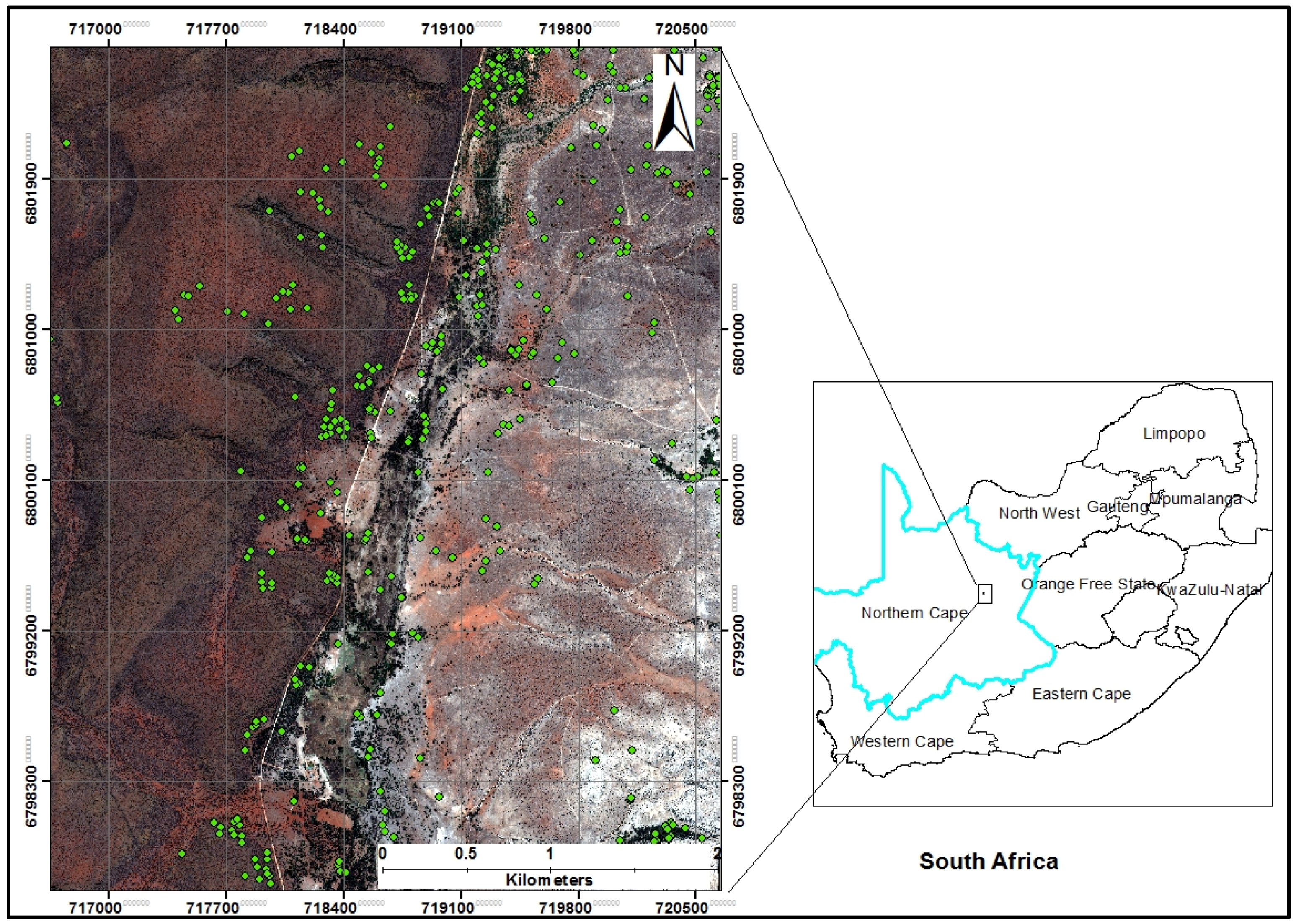
2.1. Study Area

The Northern Cape Province is a vast area covering 363,203 km², which is nearly a third of South Africa’s land area. The province is classified as a dry arid region with fluctuating temperatures and varying topographies consisting of 6 biomes [16]. Savanna and desert biomes dominate the northern part, while the west is dominated by the succulent karroo biome. The central part of the province is dominated by the Nama karroo biome. The study area is situated in the northwestern part of the province and is about 5 km from the small town of Griekwastad and 170 km from the city of Kimberley. The study area (Figure 1) covers plains with a variety of acacia, such as buffalo-thorn jujube (Ziziphus mucronata), camel thorn (Acacia erioloba), sweet thorn acacia (Acacia karroo) and black thorn acacias (Acacia mellifera), and a mixture of grasses, such as Kalahari coach (Stipagrostis amabilis), giant stick grass (Aristida meridionalis) and Lehmann’s lovegrass (Eragrostis lehmanniana) dominating the grassy plains [49]. The main activity in the study area is animal farming, mainly grazing from cattle and goats. Horses and donkeys are also prevalent in the area and are used as a cheap mode of transportation. These animals ingest the nutritious seed pods of mesquite and excrete viable seeds in their droppings, thus helping to spread mesquite over shorter distances, enabling extremely dense invasions of mesquite. As long as the seeds are not damaged by chewing, the process of digestion actually helps germination, especially since the seeds are deposited in moist, nutrient-rich dung [2].

Figure 1. A true-color composite WorldView2 image showing the location of the study area and some of the field samples.

Figure 1. A true-color composite WorldView2 image showing the location of the study area and some of the field samples.

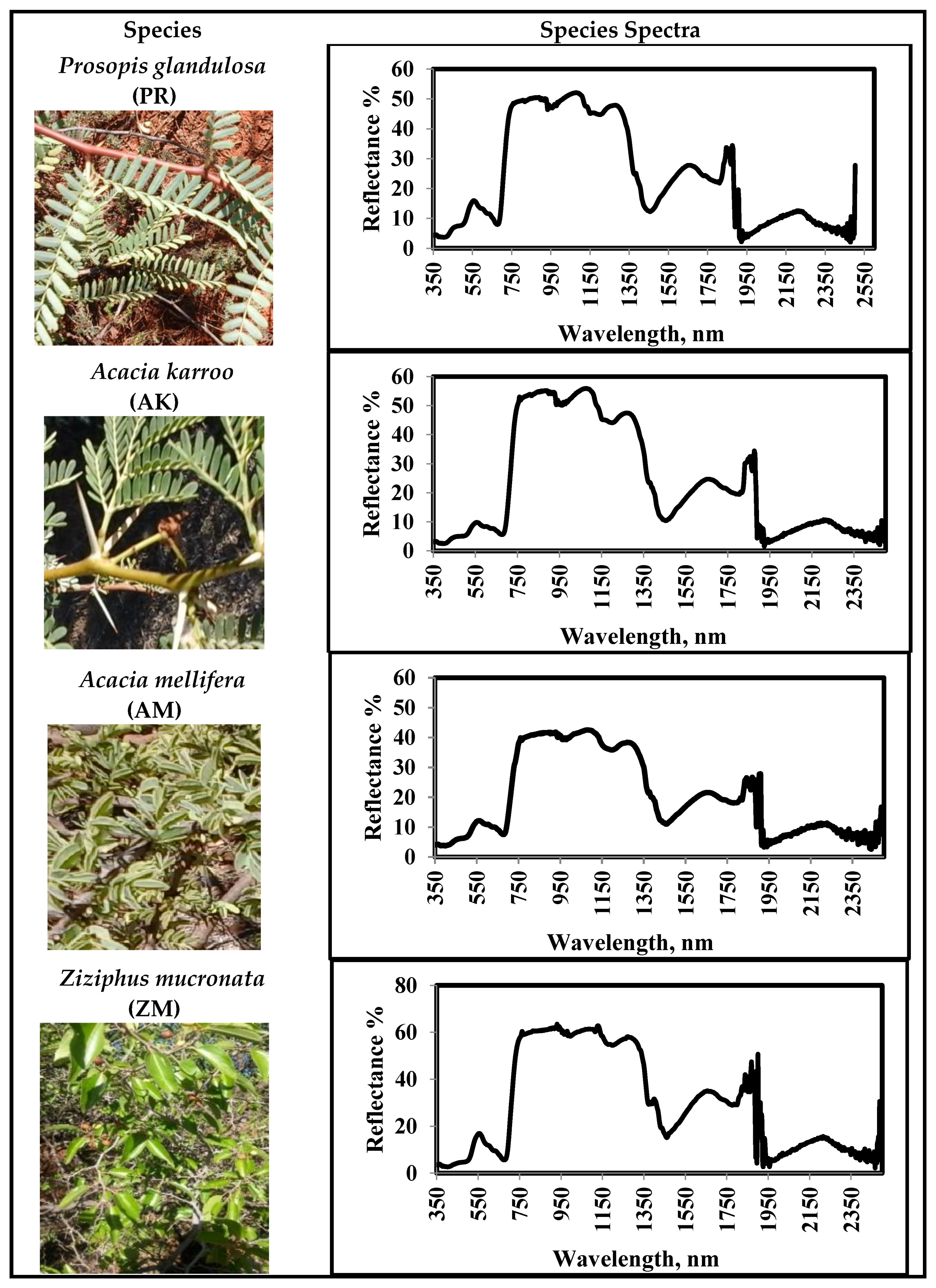
2.2. Identification of Mesquite and Other Co-Existent Tree Species

The most common tree species associated with mesquite in the area were identified in the field in summer of 2015 through field surveys [31]. In total, three main co-existent species associated with Prosopis glandulosa have been identified as the most common tree species, and these are Acacia karroo, Acacia mellifera and Ziziphus mucronata. Color digital photographs of the species were taken, and the collection of samples from each of the species, including mesquite, was sent to the C. E. Moss Herbarium Department at the School of Animal, Plant and Environmental Sciences, University of the Witwatersrand, to confirm the species identification. Acacia karroo, Acacia mellifera and Ziziphus mucronata are all indigenous plants to South Africa. They are spread throughout the country, but are most dominant in the North-West, Limpopo and Northern Cape Provinces of South Africa.

Acacia mellifera, which is known as black thorn in southern Africa, usually occurs as a multi-stemmed shrub up to 3 m high, and sometimes, it can grow as a tree to a height of 7 m [50]. The species is well adapted to dry and arid environmental conditions, and it may grow in a variety soil types, ranging from Kalahari sands to heavy and clayey soil [51].

Acacia karroo is known as sweet thorn, and it is widely distributed across different habitats of the South African region, including dry thornveld, river valley scrub, bushveld, woodland, grassland, river banks and coastal dunes of South Africa, Namibia, Angola, Botswana, Zambia and Zimbabwe [52]. Acacia karroo may grow as a shrub or small to medium-sized tree to a height of 12 m. It is a pioneer species and has the ability to encroach rapidly into grassland grazing areas, and it considered to be the most important woody invader of grasslands in South Africa [52].

Ziziphus mucronata, also known as ber, is a tropical fruit tree species that is native to the Indo-Malaysian region of South-East Asia, southern Africa, China, Australasia and the Pacific Islands. It is a spiny, evergreen and fast-growing tree with a spreading crown, stipular spines and many drooping branches [53]. The tree may grow to heights between 3 m and 12 m. The leaves are readily eaten by camels, cattle and goats [53].

2.3. Field Spectroscopy Measurements

Following the identification of the common tree species associated with mesquite, field spectral reflectance measurements were collected at canopy level over four days from 27 to 30 March 2015 under sunny and cloudless conditions between 10:00 a.m. and 02:00 p.m. The spectral reflectances were collected from mesquite and the common tree species using the Spectral Evolution^® RS-3500 Remote Sensing Portable Spectroradiometer Bundle. The spectroradiometer has a wavelength range of 350 to 2500 nm with a spectral resolution 1 nm that is resampled from inherent spectral resolutions of 3 nm at 700 nm, 8 nm at 1600 nm and 6 nm at 2100 nm [54]. Each vegetation plot (6 m × 6 m) of Prosopis and its co-existent species was sampled by cutting three to six branches from the top canopy. Piles of the branches from each sample were placed randomly on top of black thick cardboard, and the leaf reflectance was immediately measured at a nadir-looking angle at approximately 25 cm above the branches [55]. In order to derive representative reflectance spectra for each canopy (Figure 2), about 15 to 20 measurements were collected from each pile of branches by moving randomly over each canopy. Due to interferences, such as a change in atmospheric conditions, as well as irradiance of the Sun, a white reference spectral measurement was used every 10 to 20 measurements on the calibration panel to counterbalance any changes. The spectral measurements (15 to 20) from each plot were then averaged to represent the spectral reflectance of each vegetation plot (Figure 2). In total, 498 vegetation plots were sampled; 133 for Prosopis glandulosa, 108 for Acacia karroo, 133 for Acacia mellifera and 124 for Ziziphus mucronata (Table 1). In addition to the field spectral measurements, metadata giving information of general weather conditions, land cover class and coordinates were recorded for each point measured by the spectroradiometer [56].

Figure 2. Images and spectra of Prosopis glandulosa and its co-existent species.

Figure 2. Images and spectra of Prosopis glandulosa and its co-existent species.

Table 1. Sample plots of Prosopis glandulosa and its co-existent species.

Species	Training Samples (70%)	Test Samples (30%)	Total Samples
Prosopis glandulosa (PR)	93	40	133
Acacia karroo (AK)	76	32	108
Acacia mellifera (AM)	93	40	133
Ziziphus mucronata (ZM)	87	37	124

Table 1. Sample plots of Prosopis glandulosa and its co-existent species.

Species	Training Samples (70%)	Test Samples (30%)	Total Samples
Prosopis glandulosa (PR)	93	40	133
Acacia karroo (AK)	76	32	108
Acacia mellifera (AM)	93	40	133
Ziziphus mucronata (ZM)	87	37	124

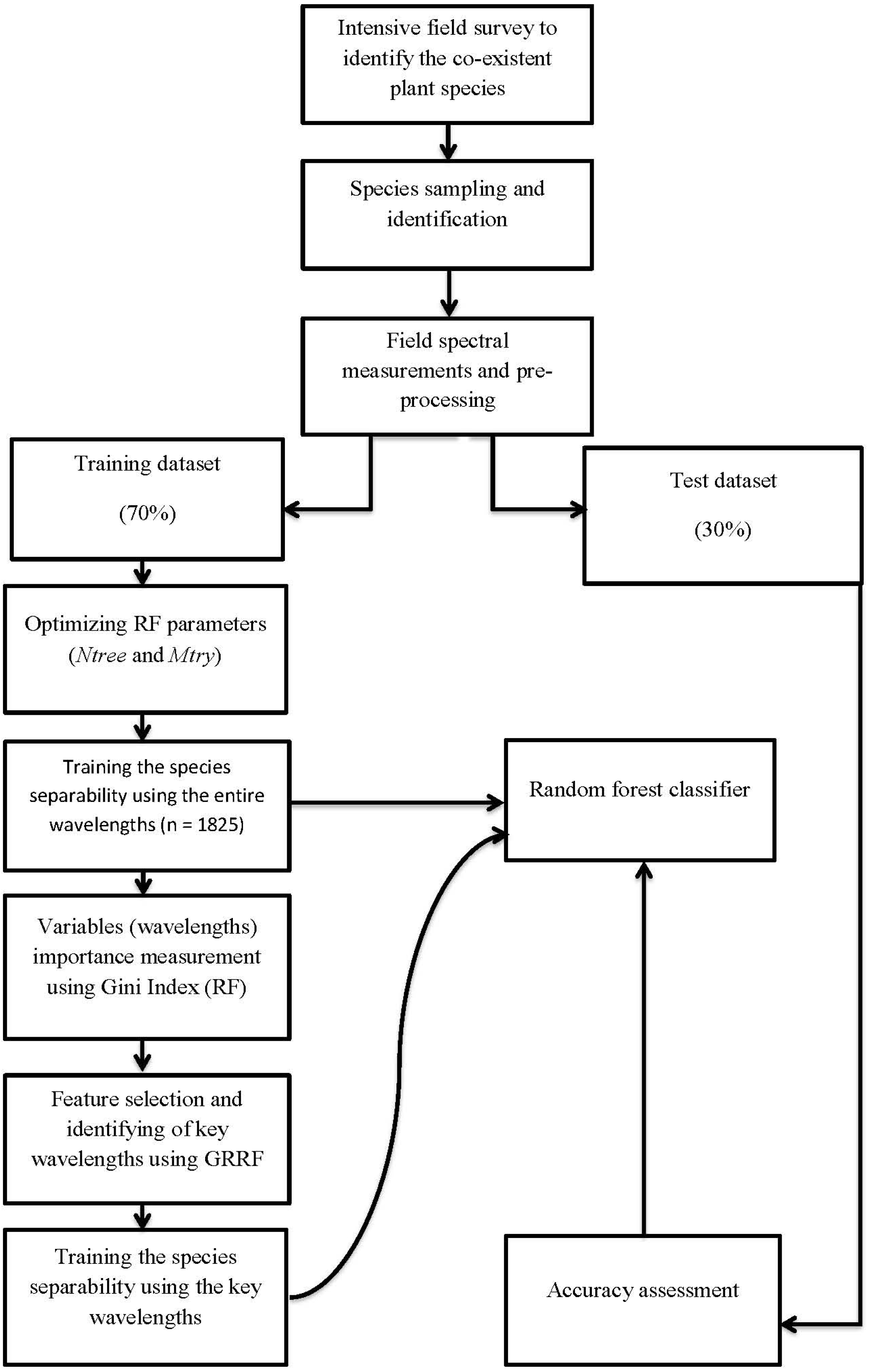
2.4. Field Spectroscopy Data Analysis

Due to noise in the reflectance spectra mainly caused by atmospheric water absorption [57], reflectance values of 325 wavelengths from three spectral regions, between 904.5 and 994.5 nm (100 bands), between 1807.2 and 2027.7 nm (90 bands) and between 2182.4 and 2503.4 nm (135 bands), were removed from the species spectra. Thus, only 1825 wavelengths were used for the spectral analysis. To reduce the “curse of dimensionality” of hyperspectral data, traditional random forest (RF) [43] and the new guided regularized random forest (GRRF) developed by Deng and Runger [47] were adapted for variable importance measurements and feature selection, respectively (Figure 3).

Figure 3. Flowchart describing the random forest (RF) and guided regularized random forest (GRRF) models used in this study.

Figure 3. Flowchart describing the random forest (RF) and guided regularized random forest (GRRF) models used in this study.

2.5. Random Forest Classifier and Variable Importance Measurement

Over the last decade, the random forest algorithm (RF) has been increasingly used to provide a new means of classifying multispectral and hyperspectral remote sensing data for different applications. RF is an ensemble decision trees developed by Breiman [43] in the field of machine learning to improve the classification and regression trees (CART). The algorithm combines bootstrap sampling to construct a large set of decision trees based on model aggregation ideas. Each tree contributes with a single vote for the assignment of the most frequent class to the input data. The two sources of randomness include: random inputs and random features. The algorithm basically benefits from two powerful techniques; bagging and random subspace selection [58]. Firstly, random forest builds many binary decision trees (ntree) to enhance the diversity of the classification trees using several bootstrap samples with replacement that are drawn from the original observations. Each single decision tree contributes with a single vote for the assignment of the most frequent class to the input data. The true classification is determined in accordance with the maximum number of votes from the collection of trees. The samples that are not in the bootstrap sample are called the out-of-bag (OOB) sample. The OOB sample (about 30% of the total data) can be used to estimate the misclassification error and variable importance. Secondly, at each node, a given number of input variables (mtry) is randomly chosen from a random subset of the features. To ensure a lower similarity (i.e., diversity) between the individual trees and, thus, a low bias, each single tree is grown without pruning on the original bootstrap sample [43,58,59]. To improve the classification accuracy, RF parameters (i.e., mtry and ntree) have to be optimized [43]. The default number of trees (ntree) is 500, while the default value for the number of variables (mtry) is √P, where P equals the number of predictor variables within a dataset [43].

For this study, a grid-search approach based on the OOB estimate of error was used to find the optimal combination for these two parameters [60]. The grid search value for mtry was varied from 1 to 10 with a single value interval, while the range of the grid search value for the ntree parameter was varied from 500 (default value) to 10,000 with an interval of 500 (20 steps). Additionally, random forest provides an internal measure of variable importance using three different methods, namely the number of times each variable is selected, the Gini importance and the permutation accuracy importance measure [61]. In this study, the Gini importance measure was adapted. The predictive power of each variable is quantified by a score (called Gini importance or Gini contrast), depending on the importance it gained over all of the trees in the random forest [43]. The ensemble does this by using the Gini index computed using the following Equations (1) to (3). The Gini index at a node $\phi$, denoted by $G \left(\phi \right)$, is given as:

$$G \left(\phi \right)= {\displaystyle \sum }_{c=1}^{numclass}{\widehat{\rho }}_c\left(1-{\widehat{\rho }}_c\right)$$

(1)

where ${\widehat{\rho }}_c$ is the proportion of observations belonging to class c at node $\phi$. The information gain of feature $f_i$ based on the Gini index on node $\phi$ is then computed as:

$$IG (f_i,\phi )= G \left(\phi \right)- {\alpha }_L G \left({\phi }^L\right)- {\alpha }_R G \left({\phi }^R\right)$$

(2)

where ${\phi }^L$ and ${\phi }^R$ denote the left and right child nodes respectively of node $\phi$ in a tree, and ${\alpha }_L$ and ${\alpha }_R$ are the proportions of observations in the left and right child nodes, respectively. As mentioned previously, in an RF model, a random subset of features is chosen at each node, and the feature with the highest information gain is used for splitting.

The overall importance score of feature $f_i$ is given by:

$$IS \left(f_i\right)= \frac{{{\displaystyle \sum }}_{\left\{split\left(f_i\right)\right\}}IG \left(f_i , \phi \right)}{ntree}$$

(3)

$\left\{split\left(f_i\right)\right\}$ is the set of all nodes over all trees ($ntree$), where $f_i$ is used for splitting.

Basically, variables associated with the OOB sample are randomly permuted, and classification trees are grown on the modified dataset. The permuted feature was used to predict the response and to obtain the accuracy. If the wavelength is initially important in the final prediction, the accuracy will drop significantly after the permutation. Thus, this difference in prediction accuracy with and without permuting the feature (wavelength) was used in this study to measure the importance of the feature. A key advantage of the random forest variable importance is that it not only deals with the impact of each variable individually, but also looks at multivariate interactions with other variables [62]. Several approaches, such as [63,64], have built on the above measure to identify the relevant set of features. However, they are either computationally expensive or do not find non-redundant set of features (Figure 3).

2.6. Feature Selection Using Guided Regularized Random Forest

Random forest has been intensively used to reduce the high dimensionality of hyperspectral data while returning relatively good accuracy levels [31,65,66,67]. However, these studies have shown that although RF provides insight into the importance of each variable in the classification process, it fails to automatically select the key number of variables that could yield the lowest error rate [31]. Moreover, studies have shown that random forest’s preference for a highly correlated predictor variable in identifying variables in high-dimensional spectral space has been identified as its major limitation [44,68]. To address this shortcoming, a regularization framework that can be applied to random forest (regularized random forest) and boosted trees (regularized boosted trees) was developed by Deng and Runger [47]. The regularization framework avoids selecting a new feature for splitting the data in a tree node when that feature produces similar information to the feature already selected. The regularized framework builds one model that may considerably reduce the training time. Therefore, guided regularized random forest (GRRF) is an enhanced regularized algorithm that uses the importance scores from an ordinary random forest to guide the feature selection process [47]. GRRF utilizes the raw feature importance scores obtained from an initial RF model. The parameters involved in the GRRF model were $mtry$, $ntree$ and $\tau$, which were optimized over a grid search using a 10-fold cross-validation on the training set. The importance score of a feature in RF is obtained by averaging the information gain (based on the Gini index) over all nodes across all trees obtained where the feature is used to split. For the purpose of GRRF, the raw importance scores obtained from RF are normalized for each feature using Equations (4) to (6).

$$NORM\_IS\left(f_i\right)=IS \left(f_i\right)/\left(ma{x}_{i=1}^F IS \left(f_i\right)\right)$$

(4)

Furthermore, the corresponding information gain is computed as:

$$I{G}_{GRRF} (f_i,\phi )= \{\begin{array}{c}IG \left(f_i,\phi \right) f_i \in F^{*}\\ {\mu }_{i}IG \left(f_i,\phi \right)otherwise\end{array}$$

(5)

where $F^{*}$ is the set of indices of features that were used for splitting in previous nodes. For the root node, $F^{*}$ = $\varnothing$. ${\mu }_i$ is an importance co-efficient for feature $f_i$ calculated as:

$${\mu }_i=\left(1-\tau \right)+ \tau I{G}_{GRRF} (f_i,\phi )$$

(6)

$\tau$ is the regularization constant. When $\tau$ = 0, we obtain the same results as from RF.

Relative studies have shown that GRRF is effective at selecting high quality feature subsets while maintaining predictive accuracies [47]. Interested readers are referred to, for example, Deng and Runger [45], Deng [46] and Deng and Runger [47] for comprehensive descriptions of GRRF theory, the principles and mathematical formulation.

2.7. Accuracy Assessment

The accuracy of the RF classifier was assessed using the independent test dataset (30%) (Figure 3). OOB, which provided an unbiased estimate of the internal RF error, was used to assess the misclassification. A confusion matrix was subsequently constructed to compute the overall accuracy (OA), user’s accuracy (UA) and producer’s accuracy (PA) as criteria for evaluating the generalization ability (accuracy) of the RF classifiers [69]. OA is a ratio (%) between the number of correctly-classified samples and the number of test samples, while UA represents the likelihood that a sample belongs to a specific class and the classifier accurately assigns it such class. PA expresses the probability of a certain class being correctly recognized.

3. Results

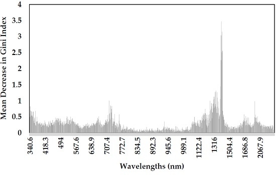
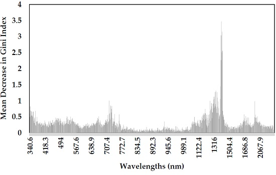
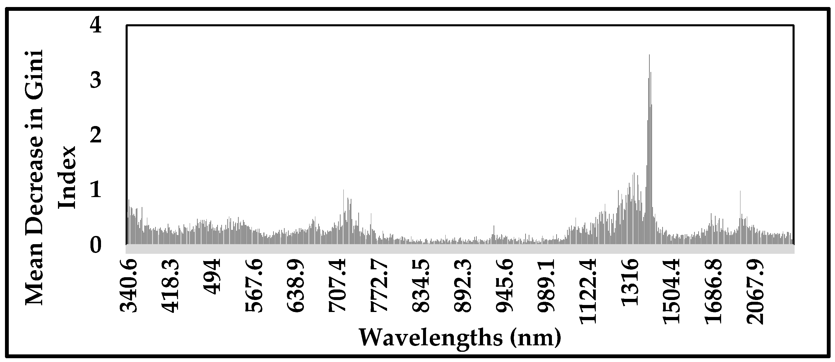
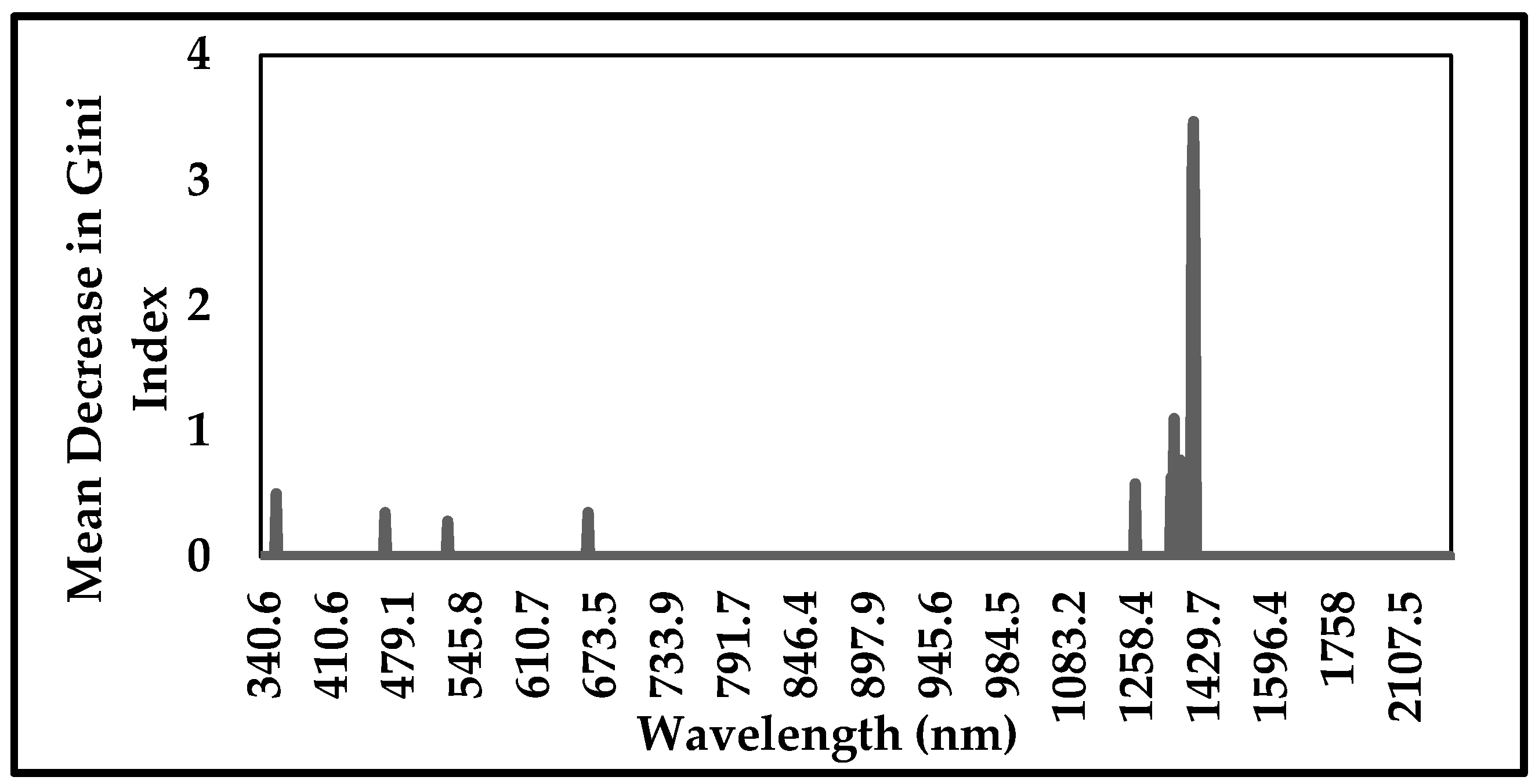
3.1. Variables Importance Measurement and Selection

The ordinary RF classifier was able to determine the importance of each wavelength in discriminating between the four species, namely Prosopis glandulosa, Acacia karroo, Acacia mellifera and Ziziphus mucronata, as shown in Figure 4. Based on the mean decrease in the Gini index, the most important wavelengths are located across the electromagnetic spectrum. For example, the wavelengths 343.7 nm and 719.4 nm are the most important wavelengths in the visible (400 to 700 nm) and red edge (690 to 720 nm) regions, respectfully. Many of the most important wavelengths for discriminating among the species are also found in the near-infrared region. These are located between 1399.6 and 1407 nm. Figure 3 clearly indicates that the top important wavelength is located at 1410.9 nm.

Figure 4. The importance of wavelengths as measured by the traditional RF using the mean decrease in the Gini index. The most important variables are those with the highest mean index.

Figure 4. The importance of wavelengths as measured by the traditional RF using the mean decrease in the Gini index. The most important variables are those with the highest mean index.

These importance scores from the random forest were used to enable GRRF’s selection of subset wavelengths that can better discriminate between the four different species. GRRF was able to identify 11 optimal wavelengths that yield the lowest OOB error. These optimal wavelengths are located at 356.3 nm, 468.5 nm, 531.1 nm, 665.2 nm, 1262.3 nm, 1354.1 nm, 1361.7 nm, 1376.9 nm, 1407.1 nm, 1410.9 nm and 1414.6 nm (Figure 5). These wavelengths were then used as input variables for the RF classifier model to discriminate between Prosopis and co-existent species.

Figure 5. Wavelengths selected by GRRF based on the importance scores as measured by the traditional RF.

Figure 5. Wavelengths selected by GRRF based on the importance scores as measured by the traditional RF.

3.2. Accuracy Assessment

The best wavelengths selected by GRRF (n = 11) were input into the random forest classifier. The lowest OOB error of 11.41% was obtained using the best combination of ntree and mtry. The classification model yielded an overall accuracy of 88.59% using the selected wavelengths (n = 11), compared to an overall accuracy of 79.19% when the total number of wavelengths (n = 1825) was used (Table 2). A comparison between the producer and user accuracies for the two datasets is shown in Table 3 for each vegetation species.

Table 2. Confusion matrix showing the overall classification and Kappa for discrimination among the four vegetation species; Prosopis glandulosa (PR), Acacia karroo (AK), Acacia mellifera (AM) and Ziziphus mucronata (ZM). The error was calculated using the out-of-bag (OOB) method and the test dataset.

Class	Using 1825 Wavelengths					Class	Using the Selected 11 Wavelengths
	AK	AM	PR	ZM	Total		AK	AM	PR	ZM	Total
AK	25	2	3	2	32	AK	27	1	2	2	37
AM	2	34	3	1	40	AM	2	36	2	0	40
PR	4	3	30	3	40	PR	1	1	36	2	40
ZM	3	1	4	29	37	ZM	2	0	2	33	37
Total	34	40	40	35	149	Total	32	38	42	37	149
OA = 79.19%						OA = 88.59%
Kappa = 0.7201						Kappa = 0.8524

Table 2. Confusion matrix showing the overall classification and Kappa for discrimination among the four vegetation species; Prosopis glandulosa (PR), Acacia karroo (AK), Acacia mellifera (AM) and Ziziphus mucronata (ZM). The error was calculated using the out-of-bag (OOB) method and the test dataset.

Class	Using 1825 Wavelengths					Class	Using the Selected 11 Wavelengths
	AK	AM	PR	ZM	Total		AK	AM	PR	ZM	Total
AK	25	2	3	2	32	AK	27	1	2	2	37
AM	2	34	3	1	40	AM	2	36	2	0	40
PR	4	3	30	3	40	PR	1	1	36	2	40
ZM	3	1	4	29	37	ZM	2	0	2	33	37
Total	34	40	40	35	149	Total	32	38	42	37	149
OA = 79.19%						OA = 88.59%
Kappa = 0.7201						Kappa = 0.8524

Table 3. Producer’s accuracy (%) and user’s accuracy (%) of the four classes (AK, AM, PR and ZM) using all of the variables (1825 wavelengths) and the most important variables (11 wavelengths).

Class	Using 1825 Wavelengths		Class	Using 11 Wavelengths
	Producer’s Accuracy (%)	User’s Accuracy (%)		Producer’s Accuracy (%)	User’s Accuracy (%)
AK	73.53	78.13	AK	84.38	84.38
AM	85.00	85.00	AM	94.74	90.00
PR	75.00	75.00	PR	85.71	90.00
ZM	82.86	78.38	ZM	89.19	89.19

Table 3. Producer’s accuracy (%) and user’s accuracy (%) of the four classes (AK, AM, PR and ZM) using all of the variables (1825 wavelengths) and the most important variables (11 wavelengths).

Class	Using 1825 Wavelengths		Class	Using 11 Wavelengths
	Producer’s Accuracy (%)	User’s Accuracy (%)		Producer’s Accuracy (%)	User’s Accuracy (%)
AK	73.53	78.13	AK	84.38	84.38
AM	85.00	85.00	AM	94.74	90.00
PR	75.00	75.00	PR	85.71	90.00
ZM	82.86	78.38	ZM	89.19	89.19

4. Discussion

Many studies have demonstrated the importance of spatial data in managing and controlling invasive plant species [70,71,72]. Since the 1800s, the invasion of the taxa of Prosopis has posed a significant threat to species diversity and caused substantial socio-economic damages world-wide [8]. Many plant invasion control methods, namely biological, chemical and mechanical, have been tried and tested over the years to reduce the impacts of mesquite with little success, as the plant is still spreading at a rate of 8% per annum in South Africa [14,15,16]. The lack of timely and accurate spatial data on the dynamics of the spread has been one of the major challenges [73]. This is due to the complexity of the mesquite characteristics, such as biology, rapid spread and many uncertainties associated with its niche colonization [74]. This study investigated the potential use of spectroscopy data in discriminating mesquite from three co-existent species in an arid environment. Results from this study show that mesquite can be accurately discriminated from other species in an arid environment of South Africa using hyperspectral data and machine learning algorithms.

The study integrated the traditional random forest and the newly-developed guided regularized random forest for hyperspectral variable selection in a multiclass classification. The traditional RF was used successfully to provide the variable importance measures to guide the regularized feature selection process. It was expected to find that many wavelengths share similar Gini information and score at a node, due to the high autocorrelation between neighboring wavelengths (1-nm interval) [75]. However, the GRRF method reduces the high dimensionality of the hyperspectral data while ensuring that such dimensionality reduction would not cause any loss of important information relevant to the object under study [76]. Many researchers have used random forest as a dimensionality reduction tool in different hyperspectral remote sensing applications [32,58,77,78,79]. However, studies have shown drawbacks to the use of random forest as a tool to measure variable importance, as well as a variable selection method [68,80]. Therefore, in this study, we introduced a newly-developed method, which has never been tested before in hyperspectral variables selection. This newly-developed method (GRRF) was able to eliminate the irrelevant and redundant wavelengths and select key wavelengths (n = 11) out of 1825 wavelengths on one iteration with less computational processes. The previous variables selection method was based on using variable selection from random forests (varSelRF) to build multiple RF models and iterations to add feature(s) with the highest importance scores(s) (forward variables selection) or to eliminate feature(s) with the least importance scores(s) in a backward variable selection method [81,82]. Such methods are computationally expensive and are not applicable for a large number of features [47]. The selected wavelengths produced a lower OOB error than the complete feature set (n = 1825 wavelengths). It is also notable that the selected wavelengths are distributed across the entire noise-free spectrum. This is because the regularization in GRRF does not select a new feature for splitting the data in a tree node if the new feature is similar in terms of information gain to the one that was already selected [45]. Such methods allow the exploration of the rich information content in hyperspectral data across the spectrum region rather than selecting only highly correlated features with redundant information [82]. The most important wavelengths selected by GRRF were at the visible and red edge (356.3 nm, 468.5 nm, 531.1 nm and 665.2 nm) and the short-wave infra-red (1262.3 nm, 1354.1 nm, 1361.7 nm, 1376.9 nm, 1407.1 nm, 1410.9 nm and 1414.6 nm) regions of the electromagnetic spectrum. The visible region of the spectrum is greatly affected by the selective absorption of the photosynthetic pigments [83]. The red edge region is the region in which the effect of vegetation biochemicals is most relevant [68]. The short-wave infrared (SWIR) is affected by water properties associated with vegetation, such as Leaf Area Index, strong leaf or canopy liquid water absorption and macronutrients [83,84,85].

The new variable selection method used in this study was first developed and tested by Deng and Runger [47] in a binary classification. The method has also shown a competitive accuracy performance in multiclass classification in this study. Following the recommendation of Deng and Runger [47], the selected wavelengths by GRRF (n = 11) were input into the RF classifier to discriminate between the Prosopis and other species (n = 4). This was due to the fact that the trees in GRRF are not designed independently of feature selection, and they may therefore have a higher variance than RF [47]. The wavelengths selected by GRRF (n = 11) yielded high classification accuracy in the RF classifier compared to the entire wavelengths (n = 1825). This was expected due to the fact that the redundant variables in a model-based analysis decrease the performance of the classifiers, because the noise in the redundant data can cause convergence instability of the classification models [39].

This high overall accuracy achieved in this study shows the potential use of hyperspectral remote sensing for mapping Prosopis at the species level and therefore provides more detail about the spatial dynamics of the Prosopis invasion. Such details are useful for effective management of the species [73]. Previous attempts of mapping Prosopis were carried out using multispectral data, such as Landsat and some environmental data, to evaluate the susceptibility of certain areas to mesquite invasion [16]. Such approaches are suitable to characterize Prosopis invasion if the plant has large spatial coverage and, thus, are unable to discriminate the species from other vegetation species. In contrast, the use of higher spatial and spectral resolution data, such as used in this study, has a great potential in fighting the invasion of the species, since species-level identification is achieved satisfactorily.

5. Conclusions

By considering the results from the study, it can be concluded that:

• One of the major problems in controlling mesquite has been the presence of mixed stands that consist of alien Prosopis mixed and indigenous species. Prosopis glandulosa can be accurately detected from its co-existent species, namely Acacia karroo, Acacia mellifera and Ziziphus mucronata, using hyperspectral data. Such potential data could provide environmental managers and ecologists insight into the development of possible appropriate spatio-temporal management practices to better control the invasive spread of mesquite.
• The problem of high dimensionality associated with spectroscopy data processing can be reduced considerably by making use of the new-developed GRRF method. The new GRRF method created high quality feature variables for the traditional RF classifier and can thus be seen as a more efficient and effective feature selection tool to reduce the high dimensionality in spectroscopy data. However, this assertion should receive considerable additional testing and comparison with the commonly-used variable selection methods before it is accepted as a substitute for reliable high dimensionality reduction.
• The wavelengths selected by GRRF showed the greatest discriminatory power of Prosopis from other species across the spectrum regions, mainly visible, red edge and short-wave infrared regions. These wavelengths are located at 356.3 nm, 468.5 nm, 531.1 nm, 665.2 nm, 1262.3 nm, 1354.1 nm, 1361.7 nm, 1376.9 nm, 1407.1 nm, 1410.9 nm and 1414.6 nm.

Overall, the results of this study offer a potential for using remote sensing to guide the physical, biological and chemical controls of Prosopis invasion. The results of this study still however need to be tested in different landscapes to establish a good understanding of the spectral characteristic of Prosopis and other co-existent vegetation at the species level. In addition, more studies are still needed to upscale these results to airborne or space-borne sensor resolutions to determine the optimal spectral and spatial resolutions to detect Prosopis taxa. These studies should consider the canopy structures of the species, as well as the understory and soil background characteristic.

References

1. Shackleton, R.T.; Le Maitre, D.C.; Pasiecznik, N.M.; Richardson, D.M. Prosopis: A global assessment of the biogeography, benefits, impacts and management of one of the world's worst woody invasive plant taxa. AoB Plants 2014, 6. [Google Scholar] [CrossRef] [PubMed]
2. Zeila, A. Mapping and managing the spread of prosopis juliflora in Garissa County, Kenya. Ph.D. Thesis, Kenyatta University, Nairobi, Kenya, 2011. [Google Scholar]
3. Klinken, R.; Shepherd, D.; Parr, R.; Robinson, T.; Anderson, L. Mapping mesquite (prosopis) distribution and density using visual aerial surveys. Rangel. Ecol. Manag. 2007, 60, 408–416. [Google Scholar] [CrossRef]
4. Awale, A.I.; Sugule, A.J. Proliferation of Honey Mesquite (Prosopis juliflora) in Somaliland: Opportunities and Challenges. Available online: http://agris.fao.org/agris-search/search.do?recordID=SO2009100043 (accessed on 14 February 2016).
5. Lloyd, J.; Berg, E.; Badenhorst, N. Mapping the Spatial Distribution and Biomass of Prosopis in the Northern Cape Province, South Africa, with the Aid of Remote Sensing and Geographic Information Systems; Report No. GW/A/98/68; Agricultural Research Council-Institute for Soil, Climate and Water: Pretoria, South Africa, 2002. [Google Scholar]
6. Pasiecznik, N.M.; Felker, P.; Association, H.D.R. The'prosopis Juliflora'-'Prosopis Pallida'complex: A Monograph; HDRA: Coventry, UK, 2001. [Google Scholar]
7. Geesingis, D.; Al Khawlani, M.; Abba, M.L. Management of introduced prosopisspecies: Can economic exploitation control an invasive species? Unasylva 2004, 217, 36–44. [Google Scholar]
8. Zimmermann, H. Biological control of mesquite, prosopis spp.(fabaceae), in South Africa. Agric. Ecosyst. Environ. 1991, 37, 175–186. [Google Scholar] [CrossRef]
9. Ghazanfar, S. Invasive prosopis in Sultanate of Oman. Aliens 1996, 3, 10–11. [Google Scholar]
10. Chikuni, M.; Dudley, C.; Sambo, E. Prosopis glandulosa torrey (leguminosae-mimosoidae) at Swang'oma, Lake Chilwa Plain: A blessing in disguise? Malawi J. Sci. Technol. 2005, 7, 10–16. [Google Scholar]
11. Choge, S.; Clement, N.; Gitonga, M.; Okuye, J. Status Report on Commercialization of Prosopis Tree Resources in Kenya; KEFRI: Nairobi, Kenya, 2012. [Google Scholar]
12. Laxén, J.P. Is Prosopis A Curse or A Blessing?: An Ecological Economic Analysis of An Invasive Alien Tree Species in Sudan; Tropical Forestry Reports; University of Helsinki: Helsinki, Finland, 2007. [Google Scholar]
13. Elfadl, M.A.; Luukkanen, O. Field studies on the ecological strategies of Prosopis juliflora in a dryland ecosystem: A leaf gas exchange approach. J. Arid Environ. 2006, 66, 1–15. [Google Scholar] [CrossRef]
14. Pasiecznik, N. Prosopis-pest or providence, weed or wonder tree? ETFRN 1999, 28, 14–15. [Google Scholar]
15. Versfeld, D.; Le Maitre, D.; Chapman, R. Alien Invading Plants and Water Resources in South Africa: A Preliminary Assessment; WRC report (no. TT 99/98); Water Research Commission: Pretoria, South Africa, 1998. [Google Scholar]
16. Berg, E.C.; Kotze, I.; Beukes, H. Detection, quantification and monitoring of prosopis in the Northern Cape Province of South Africa using remote sensing and GIS. South Afr. J. Geomat. 2014, 2, 68–81. [Google Scholar]
17. Le Maitre, D.C.; Richardson, D.M.; Chapman, R.A. Alien plant invasions in south africa: Driving forces and the human dimension: Working for water. South Afr. J.Sci. 2004, 100, 103–112. [Google Scholar]
18. Osmond, R. Mesquite Best Practice Manual: Control and Management Options for Mesquite (prosopis spp.) in Australia; Department of Natural Resources and Mines: Brisbane, Australia, 2003. [Google Scholar]
19. Maundu, P.; Kibet, S.; Morimoto, Y.; Imbumi, M.; Adeka, R. Impact of prosopis juliflora on kenya's semi-arid and arid ecosystems and local livelihoods. Biodiversity 2009, 10, 33–50. [Google Scholar] [CrossRef]
20. Witt, A. Impacts of invasive plants and their sustainable management in agro-ecosystems in Africa: A review. CABI Afr. 2010, 2010, 1102–1109. [Google Scholar]
21. Mwangi, E.; Swallow, B. Invasion of Prosopis Juliflora and Local Livelihoods: Case Study from the Lake Baringo Area of Kenya; World Agroforestry Centre: Nairobi, Kenya, 2005. [Google Scholar]
22. Baillie, J.; Hilton-Taylor, C.; Stuart, S.N. 2004 Iucn Red List of Threatened Species: A Global Species Assessment; IUCN: Gland, Switzerland, 2004. [Google Scholar]
23. Harding, G. Status of prosopis as a weed. Appl. Plant Sci. Toegep. Plantwet. 1987, 1, 43–48. [Google Scholar]
24. Coetzer, W.; Hoffmann, J. Establishment ofneltumius arizonensis (coleoptera: Bruchidae) on mesquite (prosopisspecies: Mimosaceae) in South Africa. Biol. Control 1997, 10, 187–192. [Google Scholar] [CrossRef]
25. Zachariades, C.; Hoffmann, J.; Roberts, A. Biological control of mesquite (prosopis species)(fabaceae) in South Africa. Afr. Entomol. 2011, 19, 402–415. [Google Scholar] [CrossRef]
26. Mampholo, R.K. To determine the extent of bush encroachment with focus on prosopis species on selected farms in the Vryburg district of north west province/by ramakgwale Klaas mampholo. Ph.D. Thesis, North-West University, Mahikeng, South Africa, 2006. [Google Scholar]
27. Nie, W.; Yuan, Y.; Kepner, W.; Erickson, C.; Jackson, M. Hydrological impacts of mesquite encroachment in the upper San Pedro watershed. J. Arid Environ. 2012, 82, 147–155. [Google Scholar] [CrossRef]
28. Hoshino, B.; Karamalla, A.; Manayeva, K.; Yoda, K.; Suliman, M.; Elgamri, M.; Nawata, H.; Yasuda, H. Evaluating the invasion strategic of mesquite (prosopis juliflora) in eastern Sudan using remotely sensed technique. J. Arid Land Stud. 2012, 22, 1–4. [Google Scholar]
29. Barry, P.; Mendenhall, J.; Jarecke, P.; Folkman, M.; Pearlman, J.; Markham, B. EO-1 hyperion hyperspectral aggregation and comparison with EO-1 advanced land imager and landsat 7 ETM+. Proc. IEEE 2002. [Google Scholar] [CrossRef]
30. Liew, S.C.; Chang, C.W.; Lim, K.H. Hyperspectral land cover classification of EO-1 hyperion data by principal component analysis and pixel unmixing. Proc. IEEE 2002. [Google Scholar] [CrossRef]
31. Adam, E.; Mutanga, O.; Rugege, D.; Ismail, R. Discriminating the papyrus vegetation (cyperus papyrus l.) and its co-existent species using random forest and hyperspectral data resampled to hymap. Int. J. Remote Sens. 2012, 33, 552–569. [Google Scholar] [CrossRef]
32. Artigas, F.; Yang, J. Hyperspectral remote sensing of marsh species and plant vigour gradient in the New Jersey Meadowlands. Int. J. Remote Sens. 2005, 26, 5209–5220. [Google Scholar] [CrossRef]
33. Cho, M.A.; Sobhan, I.; Skidmore, A.K.; de Leeuw, J. Discriminating species using hyperspectral indices at leaf and canopy scales. Int. Arch. Spat. Infor. 2008, 2008, 369–376. [Google Scholar]
34. Fung, T.; Ma, F.Y.; Sui, W.L. Hyperspectral data analysis for subtropical tree species identification. In Proceedings of the 1999 ASPRS Annual Conference, Portland, OR, USA, 2–6 June 1999.
35. Kumar, L.; Skidmore, A.K. Use of derivative spectroscopy to identify regions of difference between some australian eucalypt species. In Proceedings of 9th Australasian Remote Sensing and Photogrammetry Conference, Sydney, Australia, 20–24 July 1998.
36. Hsu, P. Feature extraction of hyperspectral images using wavelet and matching pursuit. ISPRS J. Photogramm. Remote Sens. 2007, 62, 78–92. [Google Scholar] [CrossRef]
37. Melgani, F.; Bruzzone, L. Classification of hyperspectral remote sensing images with support vector machines. IEEE Trans. Geosci. Remote Sens. Lett. 2004, 42, 1778–1790. [Google Scholar] [CrossRef]
38. Kavzoglu, T.; Mather, P.M. The role of feature selection in artificial neural network applications. Int. J. Remote Sens. 2002, 23, 2919–2937. [Google Scholar] [CrossRef]
39. Bajcsy, P.; Groves, P. Methodology for hyperspectral band selection. Photogramm. Eng. Remote Sens. 2004, 70, 793–802. [Google Scholar] [CrossRef]
40. Shaw, G.; Manolakis, D. Signal processing for hyperspectral image exploitation. IEEE Signal Proc. Mag. 2002, 19, 12–16. [Google Scholar] [CrossRef]
41. Pal, M. Random forest classifier for remote sensing classification. Int. J. Remote Sens. 2005, 26, 217–222. [Google Scholar] [CrossRef]
42. Borges, J.S.; Marcal, A.R.S.; Dias, J.M.B. Evaluation of feature extraction and reduction methods for hyperspectral images. In Proceedings of New Developments and Challenges in Remote Sensing, Rotterdam, the Netherlands, 29 May–2 June 2006.
43. Breiman, L. Random forests. Mach. Learn. 2001, 45, 5–32. [Google Scholar] [CrossRef]
44. Strobl, C.; Boulesteix, A.; Kneib, T.; Augustin, T.; Zeileis, A. Conditional variable importance for random forests. BMC Bioinform. 2008, 9, 307. [Google Scholar] [CrossRef] [PubMed] [Green Version]
45. Deng, H.; Runger, G. Feature selection via regularized trees. 2012. [CrossRef]
46. Guided Random Forest in the RRF Package. Available online: http://arxiv.org/abs/1306.0237 (accessed on 14 February 2016).
47. Deng, H.; Runger, G. Gene selection with guided regularized random forest. Pattern Recognit. 2013, 46, 3483–3489. [Google Scholar] [CrossRef]
48. Mucina, L.; Rutherford, M.C. The Vegetation of South Africa, Lesotho and Swaziland; South African National Biodiversity Institute: Strelitzia, South African, 2006. [Google Scholar]
49. Adam, E.M.; Mutanga, O.; Rugege, D.; Ismail, R. Field spectrometry of papyrus vegetation (cyperus papyrus l.) in swamp wetlands of St Lucia, South Africa. Proc. IEEE 2009. [Google Scholar] [CrossRef]
50. Hagos, M.; Smit, G. Soil enrichment by acacia mellifera subsp. Detinens on nutrient poor sandy soil in a semi-arid Southern African savanna. J. Arid Environ. 2005, 61, 47–59. [Google Scholar] [CrossRef]
51. Smit, G.; Richter, C.; Aucamp, A. Bush encroachment: An approach to understanding and managing the problem. In Veld Management in South Africa; University of Natal Press: Scottsville, KY, USA, 1999; pp. 246–260. [Google Scholar]
52. Taylor, C.; Barker, N. Species limits in vachellia (acacia) karroo (mimosoideae: Leguminoseae): Evidence from automated issr DNA “fingerprinting”. South Afr. J. Bot. 2012, 83, 36–43. [Google Scholar] [CrossRef]
53. Priyanka, C.; Kumar, P.; Bankar, S.P.; Karthik, L. In vitro antibacterial activity and gas chromatography—Mass spectroscopy analysis of acacia karoo and ziziphus mauritiana extracts. J. Taibah Univ. Sci. 2015, 9, 13–19. [Google Scholar] [CrossRef]
54. Spectral Evolution Rs-3500_User's Manual. Available online: http://www.spectralevolution.com/applications_Validate.html (accessed on 14 February 2016).
55. Bian, M.; Skidmore, A.K.; Schlerf, M.; Wang, T.; Liu, Y.; Zeng, R.; Fei, T. Predicting foliar biochemistry of tea (camellia sinensis) using reflectance spectra measured at powder, leaf and canopy levels. ISPRS J. Photogramm. Remote Sens. 2013, 78, 148–156. [Google Scholar] [CrossRef]
56. Milton, E.; Schaepman, M.; Anderson, K.; Kneubühler, M.; Fox, N. Progress in field spectroscopy. Remote Sens. Environ. 2009, 113, S92–S109. [Google Scholar] [CrossRef]
57. Zhao, D.; Huang, L.; Li, J.; Qi, J. A comparative analysis of broadband and narrowband derived vegetation indices in predicting lai and ccd of a cotton canopy. ISPRS J. Photogramm. Remote Sens. 2007, 62, 25–33. [Google Scholar] [CrossRef]
58. Lin, X.; Sun, L.; Li, Y.; Guo, Z.; Li, Y.; Zhong, K.; Wang, Q.; Lu, X.; Yang, Y.; Xu, G. A random forest of combined features in the classification of cut tobacco based on gas chromatography fingerprinting. Talanta 2011, 82, 1571–1575. [Google Scholar] [CrossRef] [PubMed]
59. Genuer, R.; Poggi, J.-M.; Tuleau-Malot, C. Variable selection using random forests. Pattern Recognit. Lett. 2010, 31, 2225–2236. [Google Scholar] [CrossRef]
60. Tian, F.; Yang, L.; Lv, F.; Zhou, P. Predicting liquid chromatographic retention times of peptides from the drosophila melanogaster proteome by machine learning approaches. Anal. Chimic. Acta 2009, 644, 10–16. [Google Scholar] [CrossRef] [PubMed]
61. Strobl, C.; Boulesteix, A.; Zeileis, A.; Hothorn, T. Bias in random forest variable importance measures: Illustrations, sources and a solution. BMC Bioinform. 2007, 8, 25. [Google Scholar] [CrossRef] [PubMed] [Green Version]
62. Strobl, C.; Zeileis, A. Exploring the statistical properties of a test for random forest variable importance. In Compstat 2008—Proceedings in Computational Statistics, Porto, Portugal, 30 January 2008.
63. Díaz-Uriarte, R.; De Andres, S.A. Gene selection and classification of microarray data using random forest. BMC Bioinform. 2006, 7, 3. [Google Scholar] [CrossRef] [PubMed]
64. Kursa, M.B.; Rudnicki, W.R. Feature selection with the boruta package. J. Statis. Soft. 2010, 36, 1–13. [Google Scholar]
65. Vincenzi, S.; Zucchetta, M.; Franzoi, P.; Pellizzato, M.; Pranovi, F.; De Leo, G.A.; Torricelli, P. Application of a random forest algorithm to predict spatial distribution of the potential yield of ruditapes philippinarum in the Venice lagoon, Italy. Ecol. Model. 2011, 222, 1471–1478. [Google Scholar] [CrossRef]
66. Abdel-Rahman, E.M.; Ahmed, F.B.; Ismail, R. Random forest regression for sugarcane yield prediction in umfolozi, South Africa based on landsat TM and ETM+ derived spectral vegetation indices. In Sugarcane: Production, Cultivation and Uses; Goncalves, J.F., Correia, K.D., Eds.; NOVA Science Publishers, Inc: Hauppauge NY, USA, 2012; pp. 257–284. [Google Scholar]
67. Abdel-Rahman, E.M.; Ahmed, F.B.; Ismail, R. Random forest regression and spectral band selection for estimating sugarcane leaf nitrogen concentration using EO-1 hyperion hyperspectral data. Int. J. Remote Sens. 2013, 34, 712–728. [Google Scholar] [CrossRef]
68. Adjorlolo, C.; Mutanga, O.; Cho, M.A.; Ismail, R. Spectral resampling based on user-defined inter-band correlation filter: C3 and C4 grass species classification. Int. J. Appl. Earth Obs. Geoinf. 2013, 21, 535–544. [Google Scholar] [CrossRef]
69. Mather, P.; Tso, B. Classification Methods for Remotely senSed Data; CRC press/Taylor and Francis Group: London, UK, 2003. [Google Scholar]
70. Asner, G.P.; Jones, M.O.; Martin, R.E.; Knapp, D.E.; Hughes, R.F. Remote sensing of native and invasive species in Hawaiian forests. Remote Sens. Environ. 2008, 112, 1912–1926. [Google Scholar] [CrossRef]
71. Shouse, M.; Liang, L.; Fei, S. Identification of understory invasive exotic plants with remote sensing in urban forests. Int. J. Appl. Earth Obs. Geoinf. 2013, 21, 525–534. [Google Scholar] [CrossRef]
72. Amaral, C.H.; Roberts, D.A.; Almeida, T.I.; Souza Filho, C.R. Mapping invasive species and spectral mixture relationships with neotropical woody formations in southeastern Brazil. ISPRS J. Photogramm. Remote Sens. 2015, 108, 80–93. [Google Scholar] [CrossRef]
73. Wise, R.M.; Wilgen, B.W.; Le Maitre, D.C. Costs, benefits and management options for an invasive alien tree species: The case of mesquite in the northern cape, South Africa. J. Arid Environ. 2012, 84, 80–90. [Google Scholar] [CrossRef]
74. Shiferaw, H.; Teketay, D.; Nemomissa, S.; Assefa, F. Some biological characteristics that foster the invasion of prosopis juliflora (SW.) dc. At middle awash rift valley area, north-eastern Ethiopia. J. Arid Environ. 2004, 58, 135–154. [Google Scholar] [CrossRef]
75. Kumar, L.; Dury, S.J.; Schmidt, K.; Skidmore, A. Imaging spectrometry and vegetation science. In Image Spectrometry; Meer, F.D.d., Jong, S.M.D., Eds.; Kluwer Academic Publishers: London, UK, 2003; Volume 3, pp. 111–156. [Google Scholar]
76. Adam, E.; Mutanga, O. Spectral discrimination of papyrus vegetation (cyperus papyrus l.) in swamp wetlands using field spectrometry. ISPRS J. Photogramm. Remote Sens. 2009, 64, 612–620. [Google Scholar] [CrossRef]
77. Chan, J.C.; Paelinckx, D. Evaluation of random forest and adabboost tree based ensembles classification and spectral band selection for ecotope mapping airborne hyperspectral imagery. Remote Sens. Environ. 2008. [Google Scholar] [CrossRef]
78. Zhang, G.; Li, H.; Fang, B. Discriminating acidic and alkaline enzymes using a random forest model with secondary structure amino acid composition. Proc. Biochem. 2009, 44, 654–660. [Google Scholar] [CrossRef]
79. Adam, E.; Mutanga, O.; Ismail, R. Determining the susceptibility of eucalyptus nitens forests to coryphodema tristis (cossid moth) occurrence in mpumalanga, South Africa. Int. J. Geogr. Inf. Sci. 2013, 27, 1–15. [Google Scholar] [CrossRef]
80. Mansour, K.; Mutanga, O.; Everson, T.; Adam, E. Discriminating indicator grass species for rangeland degradation assessment using hyperspectral data resampled to Aisa eagle resolution. ISPRS J. Photogramm. Remote Sens. 2012, 70, 56–65. [Google Scholar] [CrossRef]
81. Ismail, R.; Mutanga, O. Discriminating the early stages of sirex noctilio infestation using classification tree ensembles and shortwave infrared bands. Int. J. Remote Sens. 2011, 32, 4249–4266. [Google Scholar] [CrossRef]
82. Adam, E.; Mutanga, O.; Abdel-Rahman, E.M.; Ismail, R. Estimating standing biomass in papyrus (cyperus papyrus l.) swamp: Exploratory of in situ hyperspectral indices and random forest regression. Int. J. Remote Sens. 2014, 35, 693–714. [Google Scholar] [CrossRef]
83. Ceccato, P.; Flasse, S.; Tarantola, S.; Jacquemoud, S.; Grégoire, J. Detecting vegetation leaf water content using reflectance in the optical domain. Remote Sens. Environ. 2001, 77, 22–33. [Google Scholar] [CrossRef]
84. Carter, G. Ratios of leaf reflectances in narrow wavebands as indicators of plant stress. Int. J. Remote Sens. 1994, 15, 697–703. [Google Scholar] [CrossRef]
85. Ghulam, A.; Qin, Q.; Teyip, T.; Li, Z.-L. Modified perpendicular drought index (MPDI): A real-time drought monitoring method. ISPRS J. Photogramm. Remote Sens. 2007, 62, 150–164. [Google Scholar] [CrossRef]