Article

Extracting Soil Water Holding Capacity Parameters of a Distributed Agro-Hydrological Model from High Resolution Optical Satellite Observations Series

1
Centre d’Etudes Spatiales de la BIOsphère (CESBIO), Université Toulouse III Paul Sabatier, 18 Avenue Edouard Belin, 31401 Toulouse, France
2
Centre National d’Etudes Spatiales (CNES), CESBIO, 31401 Toulouse, France
3
IUT “A” Paul Sabatier, site d’Auch, 24 rue d’Embaquès, 32000 Auch, France
4
INRA—UMR1069 Sol Agro et hydrosystème Spatialisation (SAS), 35000 Rennes, France
5
Agrocampus Ouest, UMR1069, SAS, 35000 Rennes, France
6
Department of Geographical Sciences, University of Maryland, College Park, MD 20742, USA
7
NASA, Goddard Space Flight Center, Greenbelt, MD 20771, USA
8
CNRS, CESBIO, 31401 Toulouse, France
9
Laboratoire Ecologie Fonctionnelle et Environnement (EcoLab), Université de Toulouse, UPS, INPT, Avenue de l’Agrobiopole, BP 32607 Auzeville-Tolosane, 31326 Castanet-Tolosan Cedex, France
10
CNRS-Ecolab, ENSAT, Avenue de l’Agrobiopole, 31326 Castanet-Tolosan Cedex, France
*
Author to whom correspondence should be addressed.
These authors contributed equally to this work.
Submission received: 12 October 2015 / Revised: 21 January 2016 / Accepted: 25 January 2016 / Published: 17 February 2016
(This article belongs to the Special Issue Remote Sensing in Precision Agriculture)

Abstract

:
Sentinel-2 (S2) earth observation satellite mission, launched in 2015, is foreseen to promote within-field decisions in Precision Agriculture (PA) for both: (1) optimizing crop production; and (2) regulating environmental impacts. In this second scope, a set of Leaf Area Index (LAI) derived from S2 type time-series (2006–2010, using Formosat-2 satellite) is used to spatially constrain the within-field crop growth and the related nitrogen contamination of surface water simulated at a small experimental catchment scale with the distributed agro-hydrological model Topography Nitrogen Transfer and Transformation (TNT2). The Soil Water Holding Capacity (SWHC), represented by two parameters, soil depth and retention porosity, is used to fit the yearly maximum of LAI (LAX) at each pixel of the satellite image. Possible combinations of soil parameters, defining 154 realistic SWHC found on the study site are used to force spatially homogeneous SWHC. LAX simulated at the pixel level for the 154 SWHC, for each of the five years of the study period, are recorded and hereafter referred to as synthetic LAX. Optimal SWHCyear_I,pixel_j, corresponding to minimal difference between observed and synthetic LAXyear_I,pixel_j, is selected for each pixel, independent of the value at neighboring pixels. Each re-estimated soil maps are used to re-simulate LAXyear_I. Results show that simulated and synthetic LAXyear_I,allpixels obtained from SWHCyear_I,allpixels are close and accurately fit the observed LAXyear_I,allpixels (RMSE = 0.05 m2/m2 to 0.2 and R2 = 0.99 to 0.94), except for the year 2008 (RMSE = 0.8 m2/m2 and R2 = 0.8). These results show that optimal SWHC can be derived from remote sensing series for one year. Unique SWHC solutions for each pixel that limit the LAX error for the five years to less than 0.2 m2/m2 are found for only 10% of the pixels. Selection of unique soil parameters using multi-year LAX and neighborhood solution is expected to deliver more robust soil parameters solutions and need to be assessed further. The use of optical remote sensing series is then a promising calibration step to represent crop growth within crop field at catchment level. Nevertheless, this study discusses the model and data improvements that are needed to get realistic spatial representation of agro-hydrological processes simulated within catchments.

Graphical Abstract

1. Introduction

Excess nitrogen fertilizer in agricultural areas is a large source of nitrogen emissions in European fresh water and raises management challenges to societies. The goal to sustain a high-performance crop production system is not always compatible with preserving resources from pollution and overexploitation. In this context, understanding and describing the functioning of cropland areas is crucial to achieve the overlapping objectives of maintaining efficient food production systems and sustainable water resource management plan.
In that scope, Precision Agriculture (PA) aims specifically at adapting fertilization practices to local context and crop requirements. It contributes to optimizing fertilizer use, i.e., the economic performance and as a consequence minimizing nitrogen loss to water bodies. PA is then identified as a set of “environmentally friendly” practices that can be part of water management strategy in agricultural areas [1].
PA relies on high spatial resolution of geo-information, i.e., the spatial resolution of the agricultural machinery intervention. High Spatial and Temporal Resolution (HSTR) Remote Sensing (RS) data have been identified early to provide useful geo-information for diagnosing restrictive growing conditions [2]. Two applications are identified: an operational monitoring of crop stressors and requirements to adapt fertilization dates and amount in space [3,4], and enhancing the understanding of the functioning of croplands areas, to quantify the spatial variability of agro-environmental variables [5,6,7] together with the heterogeneity of physical properties, especially soil characteristics [8]. The first operational application requires appropriate schedules of RS data delivery and analysis to build up and apply site-specific agricultural practices in near real-time [9]. The second consists of geo-information data analysis to better inform the crop management in the long term using process based models. For instance, crop model predictive performances of agro-environmental variables (yield, vegetation indices, and emergence date) are improved by assimilating HSTR RS data [5,6,10]. Soil texture and soil moisture can be derived from direct approaches based on remote sensing data: (1) soil texture from the top soil layer from radar data [11,12] and hyperspectral data [13,14]; and (2) soil moisture of the first centimeters from radar [15,16]. Indirect approaches have also been explored to retrieve root zone water content and depth from inverse modeling of crop model using remote sensing derived biophysical parameters of crops cover [8] and surface soil moisture [17] to improve the prediction of within-field crop yields.
Nitrogen contamination of surface water has been studied by developing coupled model approaches to represent the agro system functioning (crop model) according to the hydrological system (hydrological model) it relies on [18,19,20,21,22]. Agro-hydrological modeling approach is constructed to clearly link both agronomical processes with spatially explicit hydrological fluxes. These approaches have been widely used to simulate the nitrate contamination in agricultural area, as the nitrogen cycle highly depends on crop’s uptake and hydrological fluxes. Most of these models are spatially distributed and require spatially explicit information: soil properties, land cover, crop type, sowing and harvesting dates, and fertilizer input. They simulate infiltration, runoff and evapotranspiration from crop [23,24,25] and nutrients transfer and transformation within the catchment [19,21,26]. Generally, the calibration and validation is performed using river discharge at the outlet of the watershed, groundwater and surface water storage fluctuations, and in-stream or groundwater nitrate concentrations. Crop productivity simulated by the crop model can be validated using basin averaged yields [26].
This spatially explicit modeling approach of water and nutrient cycles at catchment scales can make good use of HSTR RS, by detecting crop growth at catchment scales. Indeed, new satellite missions directed by European Space Agency systematically provide HSTR radar and optical data acquisition of cultivated areas (respectively, Sentinel-1 and -2). For instance, Sentinel-2 (S2) mission provide high spatial (10–20 m) and spectral (12 bands) resolution images of crop cover every five days everywhere. Recent studies have used spatial observations derived from satellite images to spatially represent evapotranspiration fluxes from the agricultural landuse in agro-hydrological models [27,28]. More recently, the distributed agro-hydrological model TNT2 (for Topography Nitrogen Transfer and Transformation) has been used to test new optimization procedures based on biophysical variables time series derived from S2 type time series [10]. In this previous study, Leaf Area Index (LAI) maps were derived from Formosat-2 satellite acquisition time series. They were used to compensate for the lack of a-priori spatial knowledge of the sowing date needed to simulate spatial crop growth and associated water and nitrogen transfers in a small experimental catchment. The spatial optimization of crop cover dynamics based on sowing date calibration had a non-negligible impact on predicted evapotranspiration and monthly discharge [29] and had a high impact on predicted nitrogen uptake by crops which consequently improved the prediction of nitrogen leaching in the river.
Whereas the spatial calibration of agricultural practices was done at the crop field level, LAI derived from satellite and field observation series show a high spatial heterogeneity within crop field, which can vary from 1 to 4 m2/m2 in within a few tens of meters. These heterogeneities are related to local soil and hydrological conditions affecting the crop growth rather than the climatic variability or fertilization rates applied within the crop field. The present work starts from this observation and is built upon this previous model calibration. Here we explore the water stress factor impacts on crop growth by setting the local Soil Water Holding Capacity (SWHC), i.e., the maximum quantity of water storage in soils and available for plant growth, which is partly driving the water fluxes from soil evaporation and crop transpiration. A previous study using the land surface model ISBA-A-gs [30] have already been evaluated regarding the water uptake of land cover by constraining the root growth and soil depth at the district level using agricultural yield statistics in France [31]. This study shows that efforts should focus on more detailed soil and root density profile description together with satellite vegetation products.
To realize this objective, we used the TNT2 model based on the crop model STICS [32], which explicitly describes dynamically the root growth, and LAI products with 8-m spatial resolution to constrain the simulated crop growth at this high spatial resolution and for a small study area. A previous global sensitivity analysis of the TNT2 model to spatial inputs and parameters was performed in an agricultural catchment in Brittany, West France, to explore the sensitivity of combined parameters on multiple output variables [33]. Among other results, it demonstrates that yields are sensitive to soil depth and parameters related to nitrogen cycle. On the contrary, spatial distribution of soil parameters gives low sensitivity with respect to water and nitrogen in-stream fluxes. The authors of this study emphasized the need to evaluate the specific sensitivity of the model to the soil spatial organization in relation to topography.
Based on this previous study, we have developed a method to integrate remotely sensed observations of crop development derived from the Formosat-2 acquisitions series with TNT2 to explore the within field variability of agro-hydrological processes such as the crop productivity, nitrogen excess and evapotranspiration fluxes. We have performed a calibration of the crop cover development at the satellite image pixel level by optimizing the maximum LAI (LAX) simulated for each year and pixel with the LAX extracted from the interpolation of LAI derived from Formosat-2 acquisition time series. Two soil parameters were used to constrain the LAX, soil depth and retention porosity, together defining the local SWHC, i.e., the maximum quantity of soil water available for plant growth. The study is thus only exploring water stress factors related to limitation of soil water availability.

2. Materials and Methods

2.1. Study Site Description

The Montoussé catchment [34] at Auradé (Gers, France) is an agricultural research site monitored since 1983 to investigate the impact of fertilizers inputs on nitrate concentrations in river water (Figure 1). The crop rotation system consists mainly of sunflower and winter wheat rotation, fertilized only with mineral fertilizers. This catchment belongs today to the French network of experimental catchments (SOERE-RBV) and to the international Critical Zone Exploration Network (CZEN).
The catchment is small, hilly and 88.5% of the surface is used for agriculture. The elevation varies between 172 and 276 meters above sea level. The substratum consists of impervious Miocene molasses deposits. Only a shallow aquifer is present, since the substratum is rather impermeable (clays) except some sand lenses that supply springs. Average daily temperature was 14.5 °C, ranging from 0 to 1 °C in winter and 29 to 30 °C in summer, giving an average potential evapotranspiration (PET) of 1020 mm·year−1. The period 2006–2010 was marked by similar annual precipitations: the mean was 664 mm·year−1, ranging from 628 to 737 mm·year−1, but hot springs and summers produced a higher PET (1039 mm·year−1). The annual discharge at the outlet is highly variable (from 6% to 33% of the rainfall during the 1985–2001 period) and represents 4% to 15% of the rainfall during the 2006–2010 study period. The climate variability in the catchment, in term of temperature and precipitation, is considered homogeneous due to its small size. Global radiation, precipitation, air temperature and PET have been measured at 800 m from the eastern margin of the experimental catchment since 2005 in addition to atmospheric flux measurements [35,36].

2.1.1. Soil Type, Hydrological Characteristics and Spatial Heterogeneity

The geological substratum is essentially impermeable, which is highly favorable to surface and subsurface runoff (hereafter called lateral flow). The subsurface flows are responsible for the major geochemical transfer of nitrate [37], metals [38] and pesticides [39] at the watershed scale, especially during storm and flood events. The soil type is predominantly non-permeable clay-limestone. A high-resolution pedological map was constructed for the experimental catchment (Figure 2a) in 2006 by Sol-Conseil and EcoLab. Twelve soil types were delineated for the catchment based on 200 auger drillings for the 325 ha. Cambisols account for 80% of the soil types in the catchment, underlined by impermeable molassic bedrock [40]. Ten soil pits have been dug to describe soil profiles of 10 soil types [41]—Annexe III in the thesis (in French). Thickness, soil bulk density, organic matter content and texture are given for each soil pit in function to depth (Table 1). Two soil types are located in the lower part of the catchment and are deeper (2 m) than soils in the middle slope (1 m depth). The deepest soils contain 2.1% organic matter in the first layer (0–20 cm), and 1.2% up to 45 cm. The other soils generally contain around 2% organic matter in the first layers, decreasing with depth to 0.5% at 30 cm. Most of the soils are made with 30%–42% clay in the first layers, increasing generally with depth, except small sandy lenses that are composed of 80% sand at 30 cm depth, located in the middle slope. The soil horizons show a high variability in term of texture. Soil depth is also highly variable in each soil type: it has, for instance, a depth of 200 and 150 cm, respectively, for Pit 1 and Pit 2 in the Cambisol calcaric colluvic soil.
This high heterogeneity of soil structure within and between soil types, highly related to the topography, is considered to explain an important part of the crop growth heterogeneity observed in the catchment.

2.1.2. LAI Monitoring from Satellite

A systematic acquisition of cloud free Formosat-2 (F2, [42]) images has been done since 2006 in the area (ground coverage of 24 km). In total, 105 images acquired between 2006 and 2010 were analyzed to derive the surface Leaf Area Index (LAI) at the resolution of F2 data (8 × 8 m resample to 5 × 5 m, using Gdal library nearest neighbor method, to the model resolution). For a given site, F2 data may be acquired every day under a constant viewing angle. A monthly acquisition of quasi cloud free images have been scheduled to sample the crop growth dynamic and to perform accurate atmospheric corrections by estimating the aerosol optical thickness using a multi-temporal method [43]. All bands of F2 images were first pre-processed for geometric, radiometric and atmospheric corrections as well as cloud and cloud-shadow filtering [44]. LAI were derived from reflectance surfaces using four spectral bands (488, 555, 650 and 830 nm) [45] using the BV-NNET tool (Biophysical Variable Neural NETwork). BV-NNET [46] is based on the inversion of a radiative transfer model, namely PROSAIL [47], using artificial neural networks. The LAI retrieval method is fully described and validated using the same F2 dataset in [48]. A main advantage of this method is that it does not require any prior calibration with in-situ measurements. Figure 1 presents a part of the F2 acquisition timeline (2006–2010) that is the study period. Four LAI maps, from 20 April 2007, 19 June 2008 and 30 June 2007 and 31 July 2008, show the time lag between maturity stage of wheat and sunflower. These products, a comprehensive observation of the crop growth dynamic, show high heterogeneity in space (inter and intra crop field) and time (between years).

2.1.3. Maximal LAI (LAX) Estimated from F2 Series

The LAI derived from F2 time series has been interpolated in a previous work at the pixel level [10] by fitting a double logistic equation against discrete satellite-derived LAI. The crop dynamics, sampled by the LAI retrieved from satellite, is expressed as a function of a cumulative daily temperature (ΣT), which is a basic formalism of crop models (Equation (2)).
L A I ( Σ T ) = K n + ( K x K n ) 1 + exp [ a × ( Σ T T i ) ] ( K x K n ) 1 + exp [ b × ( Σ T T f ) ]
Kn and Kx are, respectively, the minimum and maximum of the interpolated LAI. Ti and Tf are, respectively, the cumulative temperature when the LAI reaches Kx/2 during the growth and the senescence phases. Parameters a and b correspond to the local slope of the temperatures Tf and Ti, respectively. The LAI values simulated by the model remain stable during the maturity stage, as they correspond to dry LAI, which is different in this respect from LAI derived from the satellite observations that corresponds to a green area index and decreases quickly as leaves dry during senescence. Thus, simulated and observed LAI time series are not expected to be similar during the maturity stage, leading to difficulties in the estimation of the performances of the model on interpolated and simulated LAI profiles.
The maximum LAI (LAX), an integrative indicator of the crop development, is defined as the maximum of the interpolated function. LAX is thus defined per pixel and year. Figure 2c gives a fine but qualitative picture of the spatial crop growth heterogeneity from aerial image; the second gives a coarser but quantitative picture of the crop growth through the LAX retrieve from F2 time series. Small areas within crop field are identified in the aerial photograph, showing delay in the crop development; delays are also observable between crop fields. The LAX product shows the same spatial heterogeneity within and between crop fields.
This figure illustrates that LAX is a good quantitative descriptor of the crop productivity at the pixel size. LAX is used in this study as an integrative estimator of crop development rather than the whole LAI time-series to evaluate the performances of the model.

2.2. TNT2 Model Description and Application in the Study Site

TNT2 is a coupling approach of the crop model STICS [32] and a distributed hydrological model based on concepts developed for TopModel [49]. These concepts describe the runoff production from soil saturation within the catchment. The saturated area is linked to a local infiltration rate and sub-surface flow, which mainly depends on the catchment slope shape derived from the Digital Elevation Model (DEM) and a vertical soil hydraulic conductivity profile. The vertical profile of conductivity is defined as a transmissivity at the surface (T0 in meters), which decreases exponentially with depth (exponential decay factor, m). These two parameters are set for each soil type.

2.2.1. Spatial Water and Nitrogen Transfer Simulation

The catchment is described as a cluster of 3D columns. Each surface of the top of a column corresponds to a pixel of the Digital Elevation Model (DEM). Figure 2a presents the DEM in terms of the Topographic saturation index (TSI, Equation (2)) computed using multiple flow direction algorithms. TSI is defined as follow:
T S I = ln ( a / tan ( β ) )
where a and β are, respectively, the upstream area and the local slope.
TSI is used to distribute the water table depth under the assumption that groundwater gradients always equal topographic gradients. This hydrological scheme structures the lateral surface and subsurface flow in soil and aquifer. Each height of column is divided into two soil layers, root growth zone and a shallow aquifer layer. The soil and aquifer porosity is described as a dual porosity: the retention (micro) and drainage (macro) porosities. The porosity volume has to be set up for each layer and for each soil type that is spatially delineated by the soil raster map.
The water flow paths follow a multi-directional scheme (a pixel can flow in several pixels), which depends directly on the downstream slope calculated from the DEM (5 × 5 m, Figure 2a). This theoretical representation of hydrological routing scheme is considered more appropriate to take into account spatial processes of hydrological transfer from cells to cells such as saturated area extent [21].
Water percolation and nitrogen leaching are computed using cascading horizontal layers similar to Burns’ model [50] according to soil porosity characteristics. Both spatial soil characteristics and multi-directional scheme derived from DEM define a spatially explicit distribution of recharge and deficit of soil water saturation. In addition, cropping pattern and associated agricultural practices are given at crop field level (much larger size than the DEM grid).

2.2.2. A-priori Soil Parameters

Figure 2a represents the spatial SWHC defined in the model by both soil depth and retention porosity for two soil layers that can be explored by roots. It was set up for each soil type described by soil pits (Table 1, and in [26]).

2.2.3. Model Application in the Study Site

This spatially distributed model has been applied in the study site to simulate the spatial water and nitrogen fluxes as a function of crop rotations and fertilization practices. It was already evaluated in term of in-stream discharge and nitrogen fluxes at the outlet for the period 1985–2001 [26]. A lumped calibration of the hydrological parameters T0, m and drainage porosity was made for all the soil types on stream water discharge. Soil depth and retention porosity, hereafter called depth (meters) and micmac (from micro-porosity vs. macro-porosity, the ratio between retention porosity and drainage porosity), define the virtual SWHC. They were derived from soil pit descriptions associated with each soil type (Figure 2a). Soil nitrogen mineralization and denitrification rates are calibrated by optimizing nitrate fluxes at the outlet of the catchment.
We focused the study on the period 2005–2010, where hydrological variables together with LAI derived from F2 images are available. Discharge and nitrate concentration were continuously recorded at the outlet of the catchment area using the continuous sampling protocol described in [37]. The crop succession was derived from Registre Parcellaire Graphique (RPG) database and the crop cover supervised classification of F2 and SPOT images. The RPG is the annual farmer declarations of the land cover for crop-field blocks, a statement that is mandated by the European Common Agricultural Policy (CAP). Fertilizer amount were recorded from farmer enquiries obtained from the farmer association “association des agriculteurs d’Auradé”. A first spatial calibration of the crop emergence date using the set of LAI described previously has been performed by a re-estimation of the sowing date at the crop field level [10].

2.3. SWHC Re-Estimation Based on LAX

It is still necessary to re-estimate this “a-priori” SWHC defined by depth and micmac parameters for several reasons:
  • Soil map does not represent the real heterogeneity. Soil units correspond to a mix of soil types, within which one soil type is dominant. Heterogeneity remains within soil units, especially soil depth.
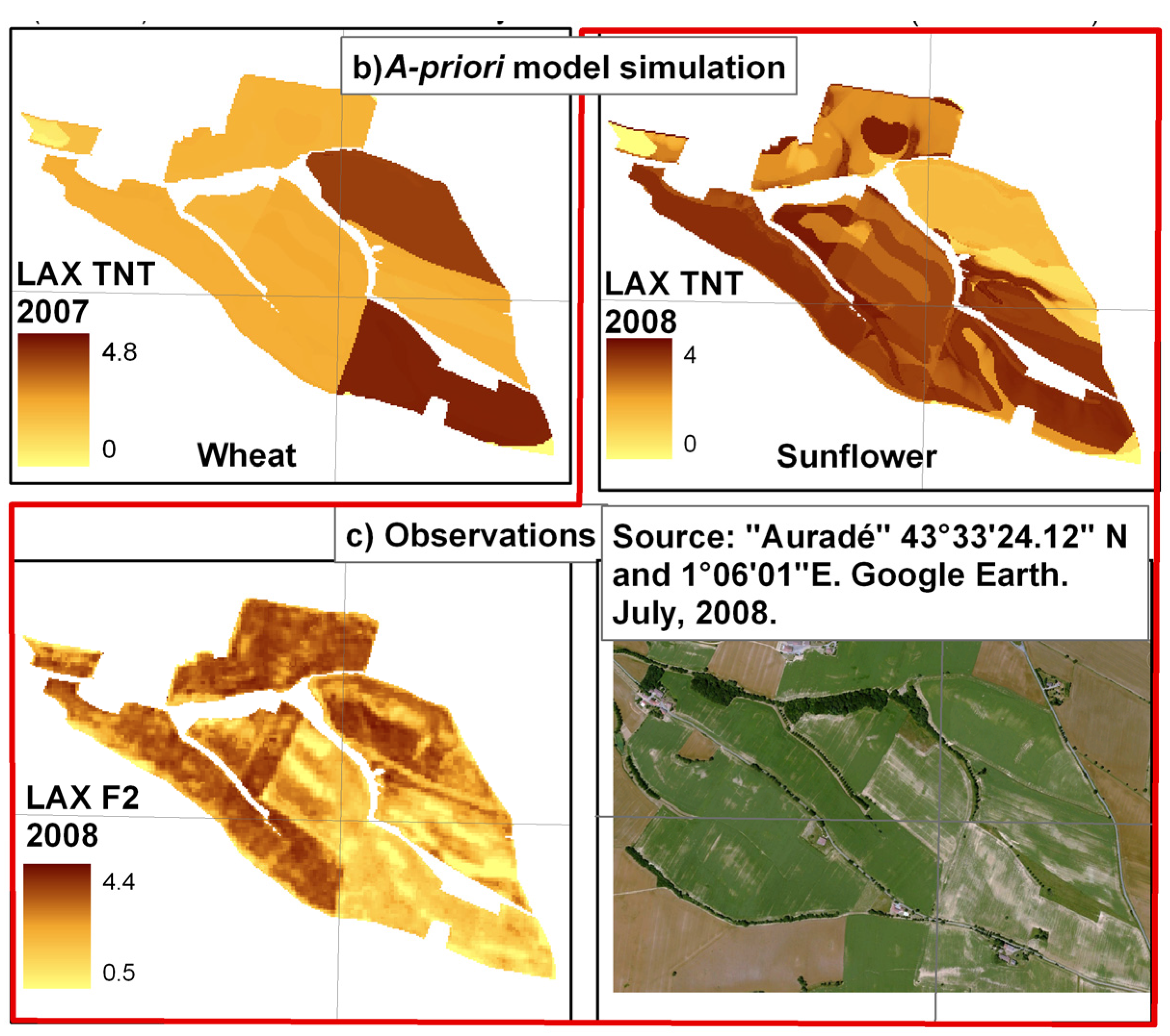
  • Soil parameters greatly impact the sunflower crop growth. Observed and simulated crop growth heterogeneity is highly influenced by soil parameters, especially for sunflower. Figure 2b shows that “a-priori” simulations from TNT2 lead to a lower heterogeneity of wheat LAX than sunflower. This heterogeneity is directly linked to the soil map delineation.
We considered the soil parameters defining SWHC (depth and micmac) as the crop growth drivers that need to be re-estimated to optimize simulated LAX derived from F2 time series. On the contrary, the soil hydrological parameters To and m are not used, even if they can dynamically impact soil water content in each computing soil layers (5 cm) by setting the drainage rate. Indeed, they also greatly impact simulated discharge at the outlet of the catchment. A spatial calibration procedure using the four soil parameters (T0, m, depth and retention porosity) can be set up at the catchment scale, but this study focuses only on few crop fields in upstream areas that are described in the next section. The choice of these soil parameters was justified by a sensitivity analysis of the simulated yield to soil depth performed in [33]. This previous study also identified a high sensitivity of crop productivity to parameters related to nitrogen cycle (mineralization rates and initial organic matter content).
Due to the high uncertainty in the knowledge of fertilization rates, the crop nitrogen related crop growth stress has been deactivated. This means that the optimized SWHC could be in certain cases impacted by the fact that nitrogen shortages have restricted observed LAX, the restriction of simulated LAX is only explained by water stress (for instance, low SWHC). Integration of nitrogen stress will be considered when uncertainty behind fertilizer input data will be minimized.

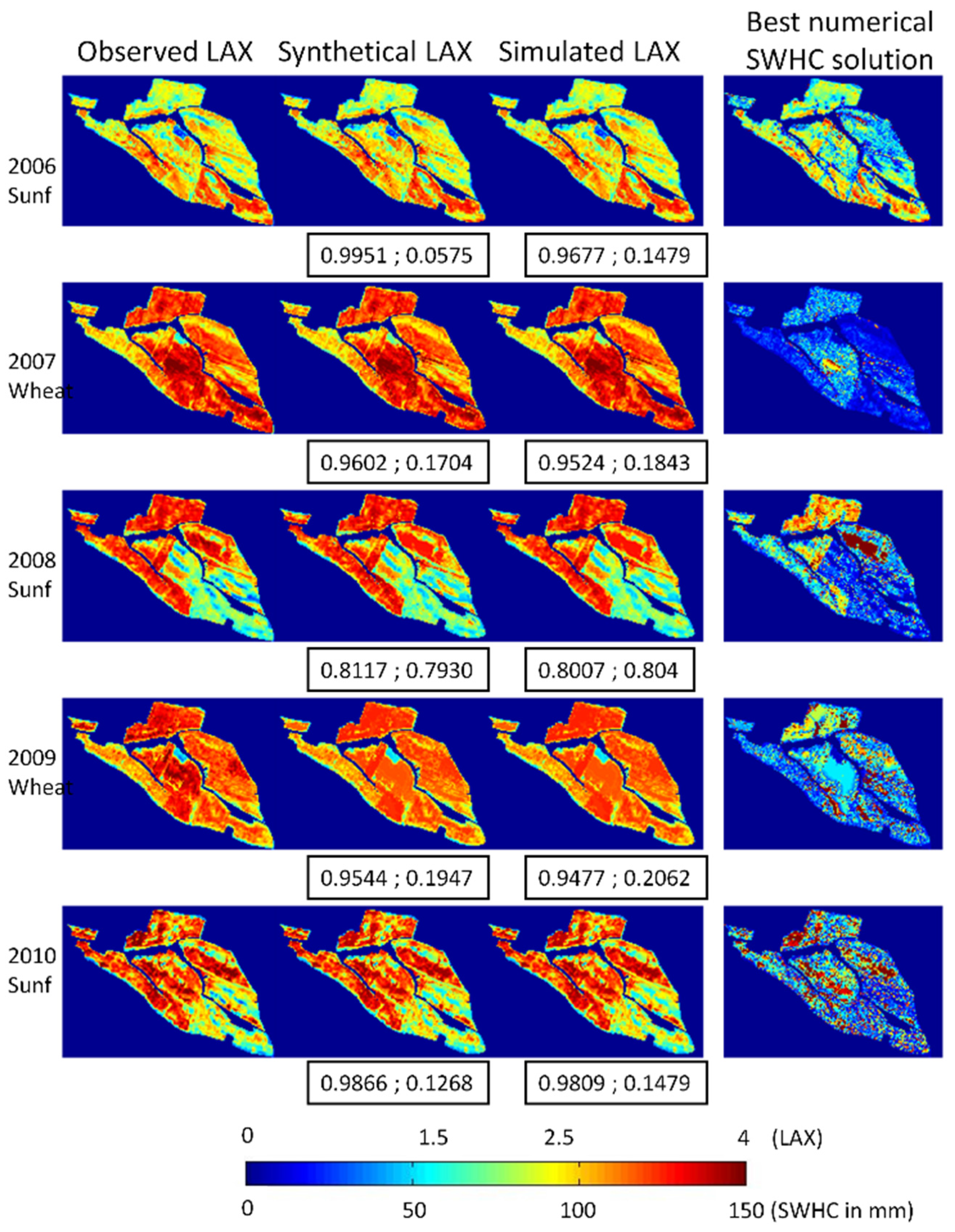
2.3.1. Generation of Synthetic LAX Based on SWHC

The selected crop fields shown in Figure 1 (underlined in red) and in Figure 2b were cultivated with wheat in 2007 and 2009 and sunflower in 2006 and 2008, and the model simulations of LAX, based on “a-priori” knowledge of SWHC from soil survey, show high variations depending on soil type delineation and hydrological pathways (derived from the multi-directional scheme based on TSI, Equation (2)). We simulated synthetic LAX for each year (2006 to 2010) in this homogeneous part in term of crops rotation of the catchment, in order to save computational time. We tested the impact of a set of realistic depth and Micmac values on LAX. Eleven soil depth values were tested, from 0.2 to 1 m, with a 0.1 step, and both 1.5 and 2 m; 14 retention porosity values were tested from 0.04 to 0.3 with intervals of 0.2 to 0.3. This corresponds to 154 pairs of parameter values that were used to force homogeneous SWHC for all the pixel in the tested area. We used a Matlab script to run in parallel the 154 TNT2 simulations and store output variables (LAX and maximum of biomass (BiomaX)) simulated for each pixel and year in a matrix. A simulation corresponds to a six-year period (2005–2010) at the catchment level (134,013 cells or modeling units). One simulation lasts for 4 to 5 h on the laboratory computing server and it took about four days to run independently the 154 simulations on eight cores. LAX and BiomaX of each growing season (2006 to 2010) are recorded at the cell size level for the studied area, corresponding to one-fifth of the catchment (33,422 cells, Figure 2). The two agronomical variables, which are good estimators of crop productivity, have spatially contrasted sensitivity to soil parameters (see sensitivity response of two pixels for both variables in Figure 3).

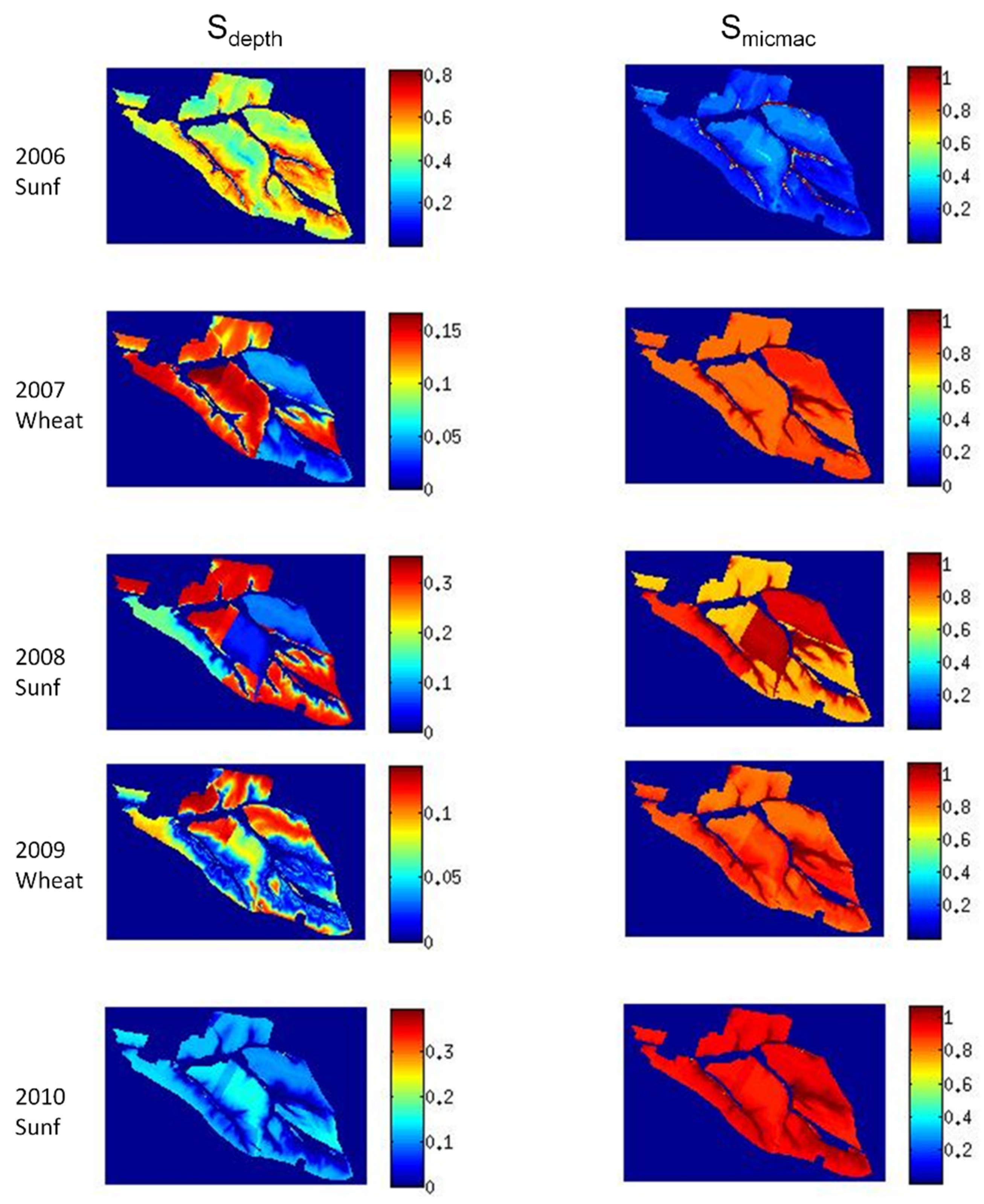
2.3.2. Spatial Sensitivity of LAX to Depth and Micmac

We used the sobol index [51], a variance decomposition method aiming at determining the part of the variance of the LAX resulting from each soil parameter value depthi, i = 1,…,11 and micmacj, j = 1,…,14. Two global measurements of the sensitivity of LAX (micmac and depth) to each input micmac and depth value tested is given by the first order Sobol index:
S d e p t h = V a r d e p t h i [ E d e p t h 1 , , d e p t h 11 L A X d e p t h i ] V a r d e p t h 1 , , d e p t h 11 [ L A X ]   f o r   i = 1 , , 11 .
S m i c m a c = V a r m i c m a c j [ E m i c m a c 1 , , m i c m a c 14 L A X m i c m a c j ] V a r m i c m a c 1 , , m i c m a c 11 [ L A X ]   f o r   j = 1 , , 14 .
These indices have been defined for each pixel and year. They are spatially represented in Figure 4 to represent the spatial and temporal sensitivity.

2.3.3. Selection Method for Numerical Best Solution of SWHC

From the 154 soil parameters pairs, we selected the closest LAX to the observed one for each year and pixel (Figure 5, respectively, columns 2 and 1). The associated LAX is called “synthetic” in the following since it was obtained from a composite of model runs. The associated soil parameter pairs are shown as the resulting best solution of SWHC in column 4. These sets of re-estimated soil parameters are then used to run the model and simulate agro-environmental variables of interest: LAX (column 3), biomass and BiomaX, daily evapotranspiration, nitrogen transfers and uptake by crops.

3. Results

3.1. Crop Growth Sensitivity

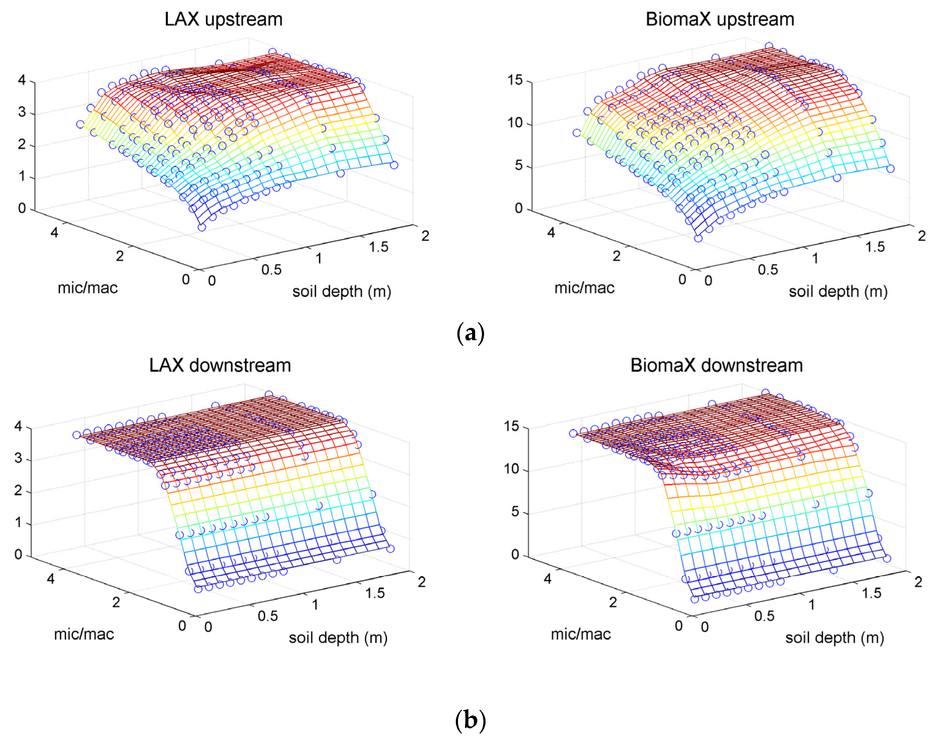
3.1.1. Sensitivity of LAX and BiomaX to Soil Parameters and TSI

A surface response of the LAX and maximum of biomass (BiomaX) to both depth and micmac is represented in Figure 3 for two locations: one in upstream (up) and one in downstream (down) areas, keeping in mind that surface responses gradually vary with the location in the slopes. Each blue circle corresponds to the result of a simulation for the cell, for the year 2006, corresponding to the sunflower.
An asymmetry of the surface response is noticeable along the increasing soil depth values for both LAX and BiomaX. Several LAX can be obtained for the same SWHC and multiple BiomaX are possibly simulated for the same LAX. Deepest soils tend to limit water stresses impacts on the biomass production during the maturity stage, when LAX is reached. A part of the downstream catchment, corresponding to the highest TSI close to the hydrological pathways, shows no sensitivity of the LAX and BiomaX to soil depth (Figure 3b). Indeed, SWHC is filled every day by the runoff and lateral flow coming from upstream parts of the catchment. Saturated conditions are simulated in these areas, whatever the soil depth value is. Crop water stress is only simulated for low retention porosity values. The model does not take into account the water excess stressors yet. These stressors are commonly observed in these clayey soils.

3.1.2. Spatial LAX Sensitivity

The LAX sensitivity to each soil parameter is represented by the Sobol indices (Sdepth and Smicmac, respectively, Equations (3) and (4)). Figure 4 shows the spatial distribution of the LAX sensitivity to the soil parameters. The soil depth explains 40% to 80% of the total sensitivity for the year 2006 (Figure 4, first line left), which is marked by dry climatic conditions in comparison to the other years. This sensitivity to soil depth decreases in low and flat areas (red colors) close to the drainage network: LAX becomes insensitive to depth in the drainage network and its neighborhood (see also Figure 3b). Water stressors are dominant this year; therefore, the soil depth is more of a limiting factor for soil water content than the retention porosity.
For the other years, sensitivity to both parameters appears to change: only 5% to 15% of the sensitivity is explained by the soil depth in 2007 (wheat in the studied part of the watershed), and is also highly dependent on the agricultural practices as the values change markedly from field crop to another. The differences of sobol indices distribution between years highlight the climatic effect on LAX sensitivity. It appears that the LAX values, simulated at a pixel level, are limited to a more or less large part of the possible LAX by stressors associated to local environment: cell position in the slope, agricultural practices, and climatic conditions. Indeed, the increase of the depth increases highly the SWHC, which globally decrease the water stress on crop growth.

3.2. Inversion of SWHC with LAX

3.2.1. Best Numerical Solutions of SWHC for One Year

We explored the capacities of the model to reproduce the spatial LAX derived from F2 image series for each year (Figure 5). Numerical best solutions of SWHC are selected at the pixel size each year. From the 154 pairs of soil parameter tested, we selected the pair giving the minimum distance between observed and synthetic LAX for each pixel (column 1 and column 2). The resulting correlation coefficient between synthetic and observed LAX are above 0.95 and RMSE below 0.2, except for the year 2008, which indicates a good ability of the model to simulate observed heterogeneity of LAX. The pairs of soil parameters used to obtain these selected synthetic LAX were used to set spatial soil parameters for each pixel (Figure 5, column 4). The model was run again with these spatial parameters to simulate LAX (Figure 5, column 3).
Contrary to synthetic LAX, which has been computed with a spatially homogeneous SWHC (i.e., soil parameters from adjacent cells were identical), simulated LAX is computed with spatial heterogeneous soil parameters. Similar LAX are obtained (column 2 and 3), although re-estimation of soil parameters induces a slight increase in the differences with observed LAX that were observed between observed and synthetic LAX. This indicates that the spatial heterogeneity of the parameters defining the SWHC have low influence on the neighborhood LAX simulations.
The model is generally able to reproduce the observed LAX heterogeneity using this spatial calibration method, except for areas where hydrological conditions are influenced by upstream fluxes rather than local soil parameters. Nevertheless, Figure 5 highlights the fact that the soil parameters selection method, based on minimal distance between observed and simulated LAX, fails in finding similar solutions between years.

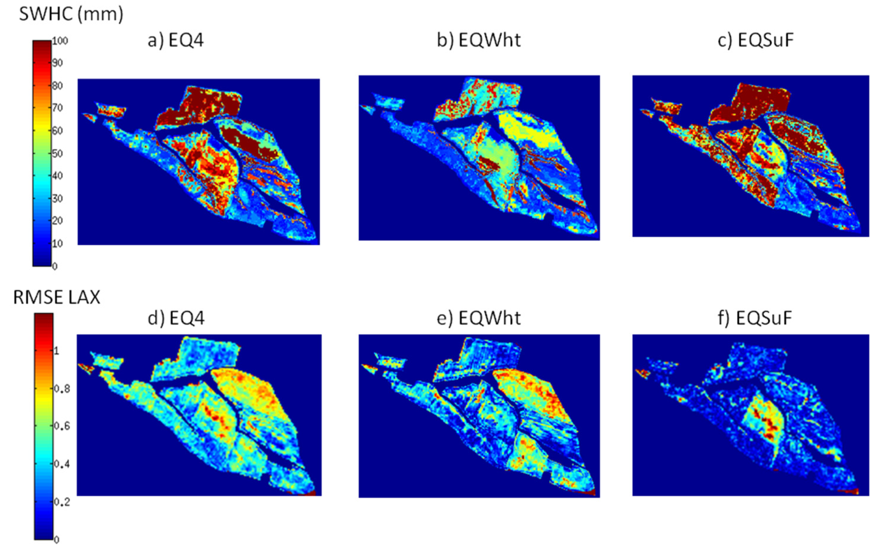
3.2.2. Multi-Year Best Numerical Solutions of SWHC

It is expected that the soil parameters are stable from year to another. However, we could not find an accurate, unique and realistic SWHC numerical solution that could fit the LAX for several years. Figure 6 shows the best numerical solutions of SWHC (up) that minimize the differences between observed and simulated LAX (in term of RMSE) for the four years (2007–2010, Figure 6a), for both wheat growth periods (i.e., only 2007 and 2009, Figure 6b), and for both sunflower growth periods (i.e., only 2008 and 2010, Figure 6c). These scenarios are named, respectively, EQ4, EQWht and EQSunF. This shows that a year-to-year constant SWHC is able to reproduce the spatial LAX variability observed from remote sensing for several years with variable error (RMSE from 0 to 1.2, RMSE = 1 corresponding to an underestimation about 25% of the LAX value). Highest errors are obtained for the wheat. In terms of SWHC, the best numerical fitting of solutions obtained for sunflower LAX is similar to the best solution for the whole period. This suggests that the sunflower is the more constraining crop for retrieving SWHC. Indeed, this is a non-irrigated summer crop. Its development highly depends on soil water content and weather conditions throughout its growth.

4. Discussion

We discuss next the basic improvements we envisage to surpass the limits described in the present study. By the way, we must keep in mind that finding a unique SWHC solution appropriate for all the study period would mean that: (1) only water stress factors explain the LAX heterogeneity observed throughout years; and (2) SWHC does not change in time, especially porosity. Expecting a unique SWHC numerical solution is not obvious, as compaction and cracking processes linked to agricultural practices and high clay content in soil profiles modify soil structure in time. Unique soil parameter calibrated from RS would be a proxy of soil properties heterogeneity impacting crop growth. This is a major improvement in the spatial agro-hydrological modeling of water and nitrogen cycle in watersheds.

4.1. Impacts of Spatial Patterns of Water and Nitrogen Uses

This new calibration step allows constraining the spatial crop nitrogen uptake, biomass production and evapotranspiration for each pixel. Based on LAX optimization, spatial patterns of simulated biomass, evapotranspiration and nitrogen content in crop are simulated within fields. Figure 7 illustrates the spatial heterogeneity of crop development for a day during the development stage of the sunflower (4 July 2006, for instance), using the best numerical solution of SWHC in 2006. Calibrating the spatial heterogeneity of LAX allows simulating LAI development and biomass production heterogeneity. On this day, LAI and biomass are not linearly related (Figure 7a,d). For a LAI value around 2, Biomass simulated values ranged from 2 to 8 t/ha. Local situations related to soil water content can lead to contrasting biomass production stressors for the same simulated LAX. This is consistent with the asymmetry observed between LAX and BiomaX sensitivity to soil parameter combination (Figure 3): several BiomaX are possibly simulated for the same LAX.
The impact of lateral flow and runoff on crop growth is highly visible on the simulated daily evapotranspiration showing that downstream areas are subjected to higher evapotranspiration rates (Figure 7). Indeed, these areas are more humid, as soil water content is highly influenced by upstream water flows. Middle slope cells with high biomass have generally low ETR during this specific summer day. This is linked to a soil water deficit that arises after the development of the crop: crop water uptake emptied the soil layers and therefore limited the ETR on this day. Figure 7e,f illustrates the relation between crop biomass and nitrogen content simulated for 4 July 2006 and the cumulative ETR simulated since January until this date. Highest Biomass production (around 8 t/ha for this day) are reached for 330 mm of ETR (Figure 7e), but high heterogeneity are simulated, depending on the importance of the evaporation fraction in the ETR, i.e., the cell position in the catchment (Figure 7b).
Crop nitrogen content also shows a strong correlation with slopes, with an increase when getting closer to the drainage network, followed by a drop of nitrogen content for crops located in cells composing this network (Figure 7c). Hydrological flows highly impact LAI growth, nitrogen uptake and biomass production in these hydrological active areas. Biomass and nitrogen content are also impacted by, respectively, sowing date and fertilization rates that are specific to each crop field, and that explain the visible delineations associated with crop field limits. In that virtual experiment, biomass production is not impacted by the fertilization rate, as the nitrogen stress factors are deactivated, i.e., the growth of biomass is enabled even in the case of nitrogen shortage. This is why there is a nonlinear relation between biomass and nitrogen content (Figure 7f): in the case of nitrogen shortage, uptake by the plant is limited but diluted in the unrestricted growing biomass, which is not realistic. Spatial calibration improves simulated LAX spatial variability, with many possibilities of biomass and nitrogen uptake estimates.

4.2. Limits and Improvements of the Model and Inversion Method

Simulations based on a-priori soil parameters can be improved in term of spatial distribution of crop productivity identified by the LAX retrieved from remote sensing series. A numerical best solution of SWHC was selected among many possible solutions for each year, based on the sensitivity of LAX to soil parameters simulated for each pixel. The differences between solutions found each year show that the selection of the optimal solution does not lead to constant soil parameters as: (1) the nitrogen stress factors behind the observed LAX are accounted for as water stress factors, and have an impact on the SWHC solution; (2) dynamic root growth simulated by the STICS model defines the maximum soil depth explored by roots but not the true soil depth; and (3) surface soil porosity changes dynamically with compaction and cracking processes.

4.2.1. Realistic SWHC

At first, the model-based estimation of the SWHC was made on the observed crop growth descriptor (LAX). The SWHC derived from one year of LAX corresponds to a volume of water used by the crop in the soil depth explored by roots. Therefore we believe that the SWHC cannot at this stage correspond to a good descriptor of the soil structure. Methods based on several years of LAI observation, together with SWHC field measurements and other remotely sensed agro-environmental variables (biomass, soil moisture), are expected to obtain more realistic physical soil parameters retrieval.
The re-estimation of “a-priori” soil descriptions impacts the crop growth and nitrogen excess at a catchment scale. The model is able to better reproduce the crop productivity descriptor, the LAX derived from remote sensing series. Nevertheless, new questions arise from this spatial calibration, especially the issue of equifinality. There are multiple combinations leading to similar LAX for each pixel. For instance, there are 50 pairs of parameter on average that lead to very small differences (<0.2) between simulated and observed LAX, varying between 0 to 154 pairs throughout pixels. The number of numerical solutions in each pixel varies from year to year, and common solutions decrease with the number of years taken into account. Over the five years simulated, common solutions for each pixel are found for less than 10% of the pixels constituting the study area, meaning that the model is generally not capable to simulate the LAXs observed with this threshold of precision (0.2) for the five years of crop succession with a constant set of soil parameters.

4.2.2. Limitations of this Virtual Experiment

The distributed model TNT2 does not yet take into account the orientation and slopes as an input factor for energy balance at the pixel size. Usually, standard global solar radiation (RG) measurements made for flat conditions with sensors installed on meteorological station are used to force the model. Process based crop models are sensitive to this forcing variable as both photosynthesis and potential and actual evapotranspiration are primarily driven by solar radiation [52]. In the study site, steep slopes (between 0% to 35%) and south–north orientations lead to contrasting incoming energy, depending on the location in the watershed. RG can be nearly twice as high for south oriented steep slopes compared to north oriented steep slopes. This effect has to be taken into account to obtain realistic estimations of incident energy intercepted by crops. RG spatial variation may have the opposite effect: better exposure to solar radiation may stimulate crop photosynthesis but also lead to additional water stress through higher evapotranspiration rates.
We have also neglected the nitrogen stress factors by deactivating the crop growth stress function related to nitrogen shortages. In that case, nitrogen related soil parameters that have a high influence on crop productivity [33] are not taken into account to extract SWHC parameters. Indeed, fertilizer inputs and soil organic matter mineralization are derived from “a-priori” knowledge and used as input parameters but large uncertainties remain. Hyper-spectral data acquisitions during bare ground period may offer the capacity to detect surface soil organic matter heterogeneity [53] that partly drives the heterogeneity of crop growth in the study site.
Retrieval of realistic soil parameter combinations from crop cover remote sensing series needs to take into account the spatial heterogeneity of RG, biomass and soil organic matter.

4.2.3. Spatial Interactions between Crop Growth and Hydrology

Contrary to 1D crop models which are developed at the crop field scale, such as STICS, or at the satellite image pixel level, such as Simple Algorithm For Yield Estimate (SAFY, [54]) and its modules (Simple Algorithm For Yield and Evapotranspiration estimates, SAFYE [55]), the distributed agro-hydrological model simulates the interaction between hydrological flow and crop growth to estimate the water and nutrient fluxes into surface and groundwater. In major parts of the catchment, local crop growth does not depend on both depth and retention porosity set for adjacent cells. Nevertheless, the position of each cell in the hydrological network highly impacts the crop growth sensitivity to the SWHC set for the cell.
More than that, down-slope areas exhibit specific functioning (Figure 3 and Figure 4). These areas correspond to saturated area along the drainage network when the groundwater level reaches the soil surface layers during the year. Crop growth is more influenced by the runoff and lateral flows that fill the SWHC than the soil parameters themselves. Some dominant processes in saturated area, such as water excess stressors that delay soil warming, slow down crop growth and hence limit its productivity are not taken into account yet. Furthermore, saturated area extent is derived from DEM (TSI, Equation (2)), and is not always realistic. Wetness index derived from dynamic distributed model is a better predictor of spatial distribution of saturated areas than the index derived from topography only [56]. It is important to validate this distribution derived from DEM as it highly impacts the modeling results in term of ETR and Nitrogen uptake by crops (Figure 7). Previous studies have used 1D models based on FAO-56 dual crop coefficient water balance model fed with high resolution NDVI image time series to estimate the spatial evapotranspiration fluxes in semi-arid and irrigated agrosystems [57]. Such models, based on remote sensing are not designed to simulate lateral flows and their impacts on the spatial redistribution of evapotranspiration, which could lead to very different results in the present hilly and non-irrigated context.
Further developments of the coupling approach are envisaged by monitoring these hydrologic active areas to better constrain the interactions between crop growth, hydrological fluxes and nitrogen transfers. Indeed, the use of soil moisture time series retrieved from high spatial resolution radar remote sensing can provide a spatial detection of these saturated areas [58]: valuable geo-information for improving the concepts and spatial description of interactions between the crop and hydrological model.

4.2.4. LAX and LAI Retrieval Uncertainty

LAI maps encompass an uncertainty that affect the LAX uncertainty and thus the TNT2 soil depth and retention porosity retrieval. The BV-NET model was validated at the pixel level using Elementary Sampling Units (ESU) and yielded an overall non-systematic error of 0.35 m2·m−2 (35%) [48]. However, we can notice that validation relies on indirect measurements: LAI derived from hemispherical photograph have an uncertainty of 0.56 m2·m−2 [59] that exceed those of BV-NET products. Finally, it is important to remember that LAI maps are retrieved using a self-calibrated approach and reliable Formosat-2 measurements [43], meaning that the spatial variability of the map uncertainty is uniform.
These elements can be used to set a threshold to select a pool of possible numerical solutions of SWHC for several years by taking the uncertainty of the LAI measurement into account.

5. Conclusions and Perspectives

This study is a first, promising attempt to derive spatial soil parameters of an agro-hydrological model from RS time-series with a distributed agro-hydrological model dedicated to topography-based simulation of nitrogen transfer and transformation. Within-field crop heterogeneity derived from spatial and temporal high-resolution satellite observation series are used to characterize crop growth using the Leaf Area Index at the pixel level (8 m).
It is possible to find optimal soil parameters related to the SWHC that fit the simulated LAX to the observations at the pixel level for each year and with acceptable computation time. On the contrary, unique SWHC solutions for each pixel, which limit the LAX error for the five-year period to less than 0.2 m2/m2, are found for only 10% of the pixels. Selection of unique soil parameters using multi-year LAX and neighborhood solution are expected to deliver more robust soil parameters solutions and need to be assessed further.
This study illustrates the importance of spatial calibration of SWHC, and beyond that the water stressors linked to soil and hydrological parameters, on nitrogen cycle simulation. It draws the path toward an improvement of the nitrogen cascade understanding in agricultural catchment by considering spatially nitrogen crop uptake and excess in well-monitored catchments.
From a modeling point of view, the 2D approach of the TNT2 model is considered more appropriate in this non-irrigated and hilly context than 1D model approaches that only simulate evapotranspiration considering NDVI retrieved from satellite remote sensing [57].
Several improvements of the spatial calibration method are identified before retrieving realistic soil parameters map: (1) identify realistic saturated downstream areas; (2) taking spatial variation of global radiation as a function of slope orientation into account; and (3) testing the ability to find SWHC solutions for multiple years and multiple crops from BiomaX and LAX detection. Radar detection of soil moisture and surface properties and biomass dynamics from Sentinel-1 observation series are foreseen to bring appropriate additional spatial predictors of crop growth stressors. Massive systematic satellite observations are becoming widely available thanks to the satellite missions Sentinel-1 and -2, which will provide high spatial resolution of optical and radar images with a 4–5-day frequency of overpass. These observations are foreseen to better predict the nitrogen runoff from cultivated area and future studies will focus on the importance of remote sensing in estimating nitrogen contamination of surface water by integrating the within-field heterogeneity of soil and crop functioning into agro-hydrological models.

Acknowledgments

This work has been conducted in the frame of the project Agro-hydrology from Space, co-funded by the living planet fellowship program from European Spatial Agency (ESA) and the research program BAG’AGES funded by the Agence de l’Eau Adour-Garonne (AEAG). This work has also received financial supports from CNRS-INSU Observatoire Spatial Regional (OSR) funds and both ANR ESCAPADE and ANR RUEdesSOLS research programs. We would like to warmly thank the Association des Agriculteurs d’Auradé (today Groupement des Agriculteurs de la Gascogne Toulousaine) for their cooperation. The BVEA (Bassin Versant Expérimental d’Auradé) is a regional platform of research and innovation in Midi-Pyrénées that is involved in the French SOERE Network RBV (Experimental catchment network) and in the international Critical Zone Exploration Network (CZEN). The study has been conducted by Sylvain Ferrant thanks to both CNES (the French Space Agency) post doctoral research grant and Living Planet fellowship from ESA. The authors would like to thank the CESBIO field team and computer services for their vital contribution to the work developed here.

Author Contributions

Sylvain Ferrant designed this virtual experiment, ran the model, analyzed the data and wrote the manuscript. Vincent Bustillo, Simon Gascoin, Enguerand Burel, Jordy Salmon-Monviola, Patrick Durand and Nathalie Jarosz participated in discussions during the experiment design and the evaluation of the results and gave valuable methodological advices. LAI data have been produced thanks to the support of Martin Claverie, Valérie Demarez, Eric Ceschia and Gérard Dedieu. Valuable methodological support has been provided by Tiangang Yin and Vincent Rivalland. Hydrological and hydro-chemical data have been provided by Anne Probst and Jean-Luc Probst. Ahmad Al-Bitar and Yann Kerr gave comments, suggestions to the manuscript and checked the writing.

Conflicts of Interest

The authors declare no conflict of interest.

References

  1. Bongiovanni, R.; Lowenberg-Deboer, J. Precision Agriculture and Sustainability. Precis. Agric. 2004, 5, 359–387. [Google Scholar] [CrossRef]
  2. Robert, P.C. Precision Agriculture: A challenge for crop nutrition management. Plant Soil 2002, 247, 143–149. [Google Scholar] [CrossRef]
  3. Haboudane, D.; Miller, J.R.; Pattey, E.; Zarco-Tejada, P.J.; Strachan, I.B. Hyperspectral vegetation indices and novel algorithms for predicting green LAI of crop canopies: Modeling and validation in the context of precision agriculture. Remote Sens. Environ. 2004, 90, 337–352. [Google Scholar] [CrossRef]
  4. Houlès, V.; Guérif, M.; Mary, B. Elaboration of a Nitrogen nutrition indicator for winter wheat based on Leaf Area Index and chlorophyll content for making nitrogen recommendations. Eur. J. Agron. 2007, 27, 1–11. [Google Scholar] [CrossRef]
  5. Launay, M.; Guerif, M. Assimilating remote sensing data into a crop model to improve predictive performance for spatial applications. Agric. Ecosyst. Environ. 2005, 111, 321–339. [Google Scholar] [CrossRef]
  6. Jégo, G.; Pattey, E.; Liu, J. Using Leaf Area Index, Retrieved from Optical Imagery, in the STICS Crop Model for Predicting Yield and Biomass of Field Crops. Field Crops Res. 2012, 131, 63–74. [Google Scholar] [CrossRef]
  7. Morel, J.; Bégué, A.; Todoroff, P.; Martiné, J.-F.; Lebourgeois, V.; Petit, M. Coupling a sugarcane crop model with the remotely sensed time series of fIPAR to optimise the yield estimation. Eur. J. Agron. 2014, 61, 60–68. [Google Scholar] [CrossRef]
  8. Varella, H.; Guérif, M.; Buis, S.; Beaudoin, N. Soil Properties estimation by inversion of a crop model and observations on crops improves the prediction of agro-environmental variables. Eur. J. Agron. 2010, 33, 139–147. [Google Scholar] [CrossRef]
  9. Hank, T.B.; Bach, H.; Mauser, W. Using a remote sensing-supported hydro-agroecological model for field-scale simulation of heterogeneous crop growth and yield: Application for wheat in central Europe. Remote Sens. 2015, 7, 3934–3965. [Google Scholar] [CrossRef]
  10. Ferrant, S.; Gascoin, S.; Veloso, A.; Salmon-Monviola, J.; Claverie, M.; Rivalland, V.; Dedieu, G.; Demarez, V.; Ceschia, E.; Probst, J.L.; et al. Agro-hydrology and multi temporal high resolution remote sensing: Toward an explicit spatial processes calibration. Hydrol. Earth Syst. Sci. 2014, 18, 5219–5237. [Google Scholar] [CrossRef]
  11. Ulaby, F.T.; Batlivala, P.P.; Dobson, M.C. Microwave backscatter dependence on surface roughness, soil moisture, and soil texture: Part I-bare soil. IEEE Trans. Geosci. Electron. 1978, 16, 286–295. [Google Scholar] [CrossRef]
  12. Niang, M.A.; Nolin, M.C.; Jégo, G.; Perron, I. Digital Mapping of soil texture using RADARSAT-2 polarimetric synthetic aperture radar data. Soil Sci. Soc. Am. J. 2014, 78, 673–684. [Google Scholar] [CrossRef]
  13. Kruse, F.A. Use of airborne imaging spectrometer data to map minerals associated with hydrothermally altered rocks in the Northern Grapevine Mountains, Nevada, and California. Remote Sens. Environ. 1988, 24, 31–51. [Google Scholar] [CrossRef]
  14. Ben-Dor, E.; Taylor, R.G.; Hill, J.; Demattê, J.A.M.; Whiting, M.L.; Chabrillat, S.; Sommer, S. Imaging spectrometry for soil applications. Adv. Agron. 2008, 97, 321–392. [Google Scholar]
  15. Zribi, M.; Hégarat-Mascle, S.; Ottlé, C.; Kammoun, B.; Guerin, C. Surface Soil moisture estimation from the synergistic use of the (multi-Incidence and Multi-Resolution) active microwave ERS wind scatterometer and SAR Data. Remote Sens. Environ. 2003, 86, 30–41. [Google Scholar] [CrossRef]
  16. Zribi, M.; Dechambre, M. A new empirical model to retrieve soil moisture and roughness from C-Band radar data. Remote Sens. Environ. 2003, 84, 42–52. [Google Scholar] [CrossRef]
  17. Sreelash, K.; Sekhar, M.; Ruiz, L.; Buis, S.; Bandyopadhyay, S. Improved modeling of groundwater recharge in agricultural watersheds using a combination of crop model and remote sensing. J. Indian Inst. Sci. 2013, 93, 189–207. [Google Scholar]
  18. Refsgaard, J.; Thorsen, M.; Jensen, J.; LKleeschulte, S.; Hansen, S. Large scale modelling of groundwater contamination from nitrate leaching. J. Hydrol. 1999, 211, 117–140. [Google Scholar] [CrossRef]
  19. Arnold, J.G.; Allen, P.M.; Bernhardt, G. A comprehensive surface-groundwater flow model. J. Hydrol. 1993, 142, 47–69. [Google Scholar] [CrossRef]
  20. Whitehead, P.; Wilson, E.; Butterfield, D. A semi-distributed integrated nitrogen model for multiple source assessment in catchment. Part 1. model structure and process equations. Sci. Total Environ. 1998, 210/211, 547–558. [Google Scholar] [CrossRef]
  21. Beaujouan, V.; Durand, P.; Ruiz, L.; Aurousseau, P.; Cotteret, G. A hydrological model dedicated to topography-based simulation of nitrogen transfer and transformation: Rationale and application to the geomorphology-denitrification relationship. Hydrol. Process. 2002, 16, 493–507. [Google Scholar] [CrossRef]
  22. Ledoux, E.; Gomez, E.; Monget, J.; Viavattene, C.; Viennot, P.; Ducharne, A.; Benoit, M.; Mignolet, C.; Schott, C.; Mary, B. Agriculture and groundwater nitrate contamination in the Seine Basin. The STICS-MODCOU modelling chain. Sci. Total Environ. 2007, 375, 33–47. [Google Scholar] [CrossRef] [PubMed]
  23. Viaud, V.; Durand, P.; Merot, P.; Sauboua, E.; Saadi, Z. Modeling the impact of the spatial structure of a hedge network on the hydrology of a small catchment in a temperate climat. Agric. Water Manag. 2005, 74, 135–163. [Google Scholar] [CrossRef]
  24. Ferrant, S.; Caballero, Y.; Perrin, J.; Gascoin, S.; Dewandel, B.; Aulong, S.; Dazin, F.; Ahmed, S.; Maréchal, J.C. Projected impacts of climate change on farmers’ extraction of groundwater from crystalline aquifers in South India. Sci. Rep. 2014, 4. [Google Scholar] [CrossRef] [PubMed]
  25. Perrin, J.; Ferrant, S.; Massuel, S.; Dewandel, B.; Marechal, J.C.; Aulong, S.; Ahmed, S. Assessing water availability in a semi-arid watershed of Southern India using a semi-distributed model. J. Hydrol. 2012, 460–461, 143–155. [Google Scholar] [CrossRef]
  26. Ferrant, S.; Oehler, F.; Durand, P.; Ruiz, L.; Salmon-Monviola, J.; Justes, E.; Dugast, P.; Probst, A.; Probst, J.L.; Sanchez-Perez, J.M. Understanding nitrogen transfer dynamics in a small agricultural catchment: Comparison of a distributed (TNT2) and a semi distributed (SWAT) modelling approaches. J. Hydrol. 2011, 406, 1–15. [Google Scholar] [CrossRef] [Green Version]
  27. Cheema, M.J.M.; Immerzeel, W.W.; Bastiaanssen, W. Spatial Quantification of groundwater abstraction in the Irrigated Indus Basin. Groundwater 2014, 52, 25–36. [Google Scholar] [CrossRef] [PubMed]
  28. Immerzeel, W.W.; Gaur, A.; Zwart, S.J. Integrating Remote sensing and a process-based hydrological model to evaluate water use and productivity in South Indian Catchment. Agric. Water Manag. 2008, 95, 11–24. [Google Scholar] [CrossRef]
  29. Martin, E.; Gascoin, S.; Grusson, Y.; Murgue, C.; Bardeau, M.; Anctil, F.; Ferrant, S.; Lardy, R.; LeMoigne, P.; Leenhardt, D.; et al. On the use of hydrological models and satellite data to study the water budget of river basins affected by human activities: Examples from the Garonne Basin of France. Surv. Geophys. 2016, in press. [Google Scholar]
  30. Calvet, J.-C.; Noilhan, J.; Roujean, J.-L.; Bessemoulin, P.; Cabelguenne, M.; Olioso, A.; Wigneron, J.-P. An interactive vegetation SVAT model tested against data from six contrasting sites. Agric. For. Meteorol. 1998, 92, 73–95. [Google Scholar] [CrossRef]
  31. Canal, N.; Calvet, J.-C.; Decharme, B.; Carrer, D.; Lafont, S.; Pigeon, G. Evaluation of root water uptake in the ISBA-A-Gs land surface model using agricultural yield statistics over France. Hydrol Earth Syst Sci 2014, 18, 4979–4999. [Google Scholar] [CrossRef]
  32. Brisson, N.; Mary, B.; Ripoche, D.; Jeuffroy, H.; Ruget, F.; Nicollaud, B.; Gate, P.; Devienne-Barret, F.; Antonioletti, R.; Durr, C.; et al. Stics: A generic model for the simulation of crops and their water and nitrogen balances. I. Theory and parameterization applied to wheat and corn. Agron. Paris 1998, 18, 311–346. [Google Scholar] [CrossRef]
  33. Moreau, P.; Viaud, V.; Parnaudeau, V.; Salmon-Monviola, J.; Durand, P. An approach for global sensitivity analysis of a complex environmental model to spatial inputs and parameters: A case study of an agro-hydrological model. Environ. Model. Softw. 2013, 47, 74–87. [Google Scholar] [CrossRef]
  34. BVEA. Availabel oneline: http://www.ecolab.omp.eu/bvea/ (accessed on 14 February 2016).
  35. Béziat, P.; Ceschia, E.; Dedieu, G. Carbon balance of three crop succession over two cropland sites in South West of France. Agric. For. Meteorol. 2009, 149, 1628–1645. [Google Scholar] [CrossRef] [Green Version]
  36. Tallec, T.; Béziat, P.; Jarosz, N.; Rivalland, V.; Ceschia, E. Crop’s water use efficiencies in temperate climate: Comparison of stand, ecosystem and agronomical approaches. Agric. For. Meteorol. 2013, 168, 69–81. [Google Scholar] [CrossRef]
  37. Ferrant, S.; Laplanche, C.; Durbe, G.; Probst, A.; Dugast, P.; Durand, P.; Sanchez-Perez, J.M.; Probst, J.L. Continuous measurement of nitrate concentration in a highly event-responsive agricultural catchment in South-West of France: Is the gain of information useful? Hydrol. Proc. 2012, 12, 1751–1763. [Google Scholar] [CrossRef] [Green Version]
  38. Roussiez, V.; Probst, A.; Probst, J.-L. Significance of floods in metal dynamics and export in a small agricultural catchment. J. Hydrol. 2013, 499, 71–81. [Google Scholar] [CrossRef]
  39. Taghavi, L.; Probst, J.-L.; Merlina, G.; Marchand, A.-L.; Durbe, G.; Probst, A. Flood event impact on pesticide transfer in a small agricultural catchment (Montoussé at Auradé, South West France). Int. J. Environ. Anal. Chem. 2010, 90, 390–405. [Google Scholar] [CrossRef]
  40. Macary, F.; Almeida-Dias, J.; Uny, D.; Probst, A. Assessment of the Effects of best environmental practices on reducing pesticide contamination in surface water, using multi-criteria modelling combined with a GIS. Int. J. Multicriteria Decis. Mak. 2013, 3, 178–211. [Google Scholar] [CrossRef]
  41. Perrin, A.-S. Rôle Des Fertilisants Azotés Dans L’érosion Chimique Des Bassins Versants Carbonatées: Implication Dans La Consommation de CO2 et La Composition Chimique Des Eaux de Surface. Ph.D. Thesis, Université de Toulouse, Toulouse, France, March 2008. [Google Scholar]
  42. Chern, J.S.; Wu, A.M.; Lin, S.F. Lesson learned from Formosat-2 mission operations. Acta Astronaut. 2006, 59, 344–350. [Google Scholar] [CrossRef]
  43. Hagolle, O.; Dedieu, G.; Mougenot, B.; Debaeker, V.; Duchemin, B.; Meygret, A. Correction of aerosol effects on multi-temporal images acquired with constant viewing angles: Application to formoat-2 images. Remote Sens. Environ. 2008, 112, 1689–1701. [Google Scholar] [CrossRef] [Green Version]
  44. Hagolle, O.; Huc, M.; Pascual, D.V.; Dedieu, G. A multi-temporal method for cloud detection, applied to FORMOSAT-2, VENuS, LANDSAT and SENTINEL-2 Images. Remote Sens. Environ. 2010, 114, 1747–1755. [Google Scholar] [CrossRef] [Green Version]
  45. Claverie, M.; Demarez, V.; Duchemin, B.; Hagolle, O.; Ducrot, D.; Dejoux, J.F.; Huc, M.; Keravec, P.; Béziat, P.; Fieuzal, R.; et al. Maize and sunflower biomass estimation in Southwest France using high spatial and temporal resolution remote sensing data. Remote Sens. Environ. 2012, 124, 844–857. [Google Scholar] [CrossRef] [Green Version]
  46. Baret, F.; Hagolle, O.; Geiger, B.; Bicheron, P.; Miras, B.; Huc, M.; Berthelot, B.; Nino, F.; Weiss, M.; Samain, O.; et al. LAI, fAPAR and fCover CYCLOPES Global products derived from VEGETATION. Part 1: principles of the algorithm. Remote Sens. Environ. 2007, 3, 275–286. [Google Scholar] [CrossRef] [Green Version]
  47. Jacquemoud, S.; Verhoef, W.; Baret, F.; Bacour, C.; Zarco-Tejada, P.J.; Asner, G.P.; François, C.; Ustin, S.L. PROSPECT + SAIL models: A review of use for vegetation characterization. Remote Sens. Environ. 2009, 113, 56–66. [Google Scholar] [CrossRef]
  48. Claverie, M.; Vermote, E.F.; Weiss, M.; Baret, F.; Hagolle, O.; Demarez, V. Validation of coarse spatial resolution LAI and FAPAR time series over cropland in Southwest France. Remote Sens. Environ. 2013, 139, 216–230. [Google Scholar] [CrossRef]
  49. Beven, K. Distributed modelling in hydrology: Applications of topmodel concept. Adv. Hydrol. Process. 1997, 350, 59–79. [Google Scholar]
  50. Burns, I. A model for predicting the redistribution of salts applied to fallow soils after excess of rainfall or evaporation. J. Soil Sci. 1974, 25, 165–178. [Google Scholar] [CrossRef]
  51. Sobol, I.M. Sensitivity estimates for non linear mathematical models. Math. Model. Comput. Exp. 1993, 1, 407–414. [Google Scholar]
  52. Trnka, M.; Eitzinger, J.; Kapler, P.; Dubrovský, M.; Semerádová, D.; Žalud, Z.; Formayer, H. Effect of estimated daily global solar radiation data on the results of crop growth models. Sensors 2007, 7, 2330–2362. [Google Scholar] [CrossRef]
  53. Gmur, S.; Vogt, D.; Zabowski, D.; Moskal, L.M. Hyperspectral analysis of soil nitrogen, carbon, carbonate, and organic matter using regression trees. Sensors 2012, 12, 10639–10658. [Google Scholar] [CrossRef]
  54. Duchemin, B.; Maisongrande, P.; Boulet, G.; Benhadj, I. A Simple algorithm for yield estimates: evaluation for semi-arid irrigated winter wheat monitored with green Leaf Area Index. Environ. Model. Softw. 2008, 23, 876–892. [Google Scholar] [CrossRef]
  55. Claverie, M. Estimation spatialisee de la biomasse et des besoins en eau des cultures a l’aide de donnees satellitales a hautes resolutions spatiale et temporelle: Application Aux agrosystemes du sud-ouest de la France. Ph.D. Thesis, Université de Toulouse, Toulouse, France, 2012. [Google Scholar]
  56. Grabs, T.; Seibert, J.; Bishop, K.; Laudon, H. Modeling spatial patterns of saturated areas: A comparison of the topographic wetness index and a dynamic distributed model. J. Hydrol. 2009, 373, 15–23. [Google Scholar] [CrossRef] [Green Version]
  57. Saadi, S.; Simonneaux, V.; Boulet, G.; Raimbault, B.; Mougenot, B.; Fanise, P.; Ayari, H.; Lili-Chabaane, Z. Monitoring irrigation consumption using high resolution NDVI image time series: Calibration and validation in the Kairouan Plain (Tunisia). Remote Sens. 2015, 7, 13005–13028. [Google Scholar] [CrossRef]
  58. Baghdadi, N.; Aubert, M.; Zribi, M. Use of TerraSAR-X data to retrieve soil moisture over bare soil agricultural fields. IEEE Geosci. Remote Sens. Lett. 2012, 9, 512–516. [Google Scholar] [CrossRef] [Green Version]
  59. Demarez, V.; Duthoit, S.; Baret, F.; Weiss, M.; Dedieu, G. Estimation of leaf area and clumping indexes of crops with hemispherical photographs. Agric. For. Meteorol. 2008, 148, 644–655. [Google Scholar] [CrossRef] [Green Version]
Figure 1. Study site location in southwest France and satellite time series acquisitions details. Four 8 meters resolution Leaf Area Index (LAI) products are shown: high and low LAI correspond to, respectively, well developed wheat and first growing stage sunflower in April; low LAI value for the dry wheat and high LAI for the maturity stage of sunflower in June 2007. The next year (2008), opposite location of crops are observed, implied by the sunflower and winter wheat crop succession. The area used to test the methodology corresponds to the underlined crop field in red. It corresponds to a homogeneous area in term of crop cover: sunflower in 2006, 2008 and 2010, and winter wheat in 2007 and 2009.
Remotesensing 08 00154 g001
Figure 2. Details of the Topography Nitrogen Transfer and Transformation (TNT2) model spatial input (a) with “a-priori” Soil Water Holding Capacity (SWHC) parameters derived from soil map and soil survey and the Topographic saturation index (TSI) value (Equation (1)) derived from Digital Elevation Model; (b) Simulation of maximum LAI (LAX) for the wheat (2007) and the sunflower (2008) with “a-priori” soil parameters; (c) LAX derived from satellite series and aerial photography of the sunflower crop cover in July 2008. The red polygon highlight the simulations and observations for the year 2008.
Remotesensing 08 00154 g002aRemotesensing 08 00154 g002b
Figure 3. Sunflower maximum of LAI (LAX) and biomass (BiomaX in t/ha) sensitivity to soil parameters for the year 2006: retention/drainage porosity ratio (mic/mac) and soil depth, for a pixel located in upstream area (a); and downstream area (b). Each blue circle corresponds to a TNT2 simulation.
Remotesensing 08 00154 g003
Figure 4. Sobol indices of each sensitivity surfaces of LAX for each pixel and each year (line). Sdepth and Smicmac (respectively, Equations (1) and (2)) represent the sobol sensitivity of LAX to the soil depth parameter (depth, first column) and Smicmac the sensitivity to the retention porosity parameter (micmac, micro–macro porosity ratio). The higher the value is, the higher the sensitivity is.
Remotesensing 08 00154 g004
Figure 5. Observed, synthetic and simulated LAX (in column) for each year (in line). The fourth column represents the best numerical solution of SWHC for each year selected from the best fit between synthetic LAX (second column) and observed LAX (first column). The third column shows simulated LAX after having reset soil parameters using the best numerical solution of the fourth column. Numbers in the boxes represent the correlation coefficient and the RMSE between synthetic and observed LAX (second column) and simulated and observed LAX (third column) for each year.
Remotesensing 08 00154 g005
Figure 6. The optimal SWHC derived by minimizing the distance between observed and synthetic LAX over (a) four years (2007–2010); (b) two years for winter wheat (2007 and 2009); and (c) two years in Sunflower (2008 and 2010) are presented. The RMSE computed between observed and simulated LAX is presented for each method (df). RMSE around 1 corresponds to 25% of the maximum LAI (max(LAX) = 4) observed for the studied crops.
Remotesensing 08 00154 g006
Figure 7. Sunflower development simulated for the year 2006 after reinitializing soil parameters: (a); Simulation of the biomass on 14 July 2006 with the relationship between LAI this day and Biomass (b); The corresponding evapotranspiration for this day (c); Biomass of each pixel is shown as a function of cumulative evapotranspiration from January to July (d); The corresponding N content in crop on 4 July (e); High heterogeneity between biomass and nitrogen content in sunflower is simulated because the nitrogen stress factors do not influence biomass growth in these simulations (f).
Remotesensing 08 00154 g007
Table 1. Soil types and physical characteristics in Auradé catchment (source from Sol-Conseil and EcoLab).
Soil NameSurface Proportion (%)Layers (cm)Sand (%)Silt (%)Clay (%)Organic Matter (%)C/NApparent Density
Cambisol calcaric locally endostagnic (*)31.00–2525.936.937.228.31.67
25–502936.234.81.57.41.69
50–10031.234.8340.96.81.72
>1001755.627.40.46.3-
Fluvic cambisol calcaric19.00–2021.741.436.92.18.21.52
20–4515.445.539.11.271.64
45–708.852.139.10.96.51.73
70–14011.948.639.50.96.21.6
140–1802237.540.50.75.81.53
Cambisol calcaric colluvic soil pit 110.00–2523.337.938.81.77.91.58
25–6519.736.543.80.44.51.7
65–12019.43644.60.23.11.76
120–13039.129.231.70.12.6-
130–16052.328.918.80.11.7-
160–20075.9168.10.25.8-
Cambisol calcaric colluvic soil pit 2Same soil than previous0–25-----1.67
25–6018.338.643.11.57.41.69
60–15013.639.946.50.441.72
Rendzic leptosol (molassic material)4.50–251945.435.61.58.91.74
25–4037.942.1200.35.7-
40–7036.546.317.20.48.4-
>7037.450.512.10.23.7-
Cambisol hypereutric (farmed)1.60–251837.244.82.391.33
25–8020.637.841.61.27.91.7
80–12015.23648.80.65.1-
120–15016.946.536.60.55.9-
Cambisol hypereutric (forested)Same soil than previous0–1520.636.742.75.312.2-
15–5018.736.245.11.58.4-
50–10013.735.3510.75.6-
100–15011.435.752.90.33.2-
Rendzic leptosol0.90–2070.424.714.92.110.1-
(calcaric material)>206323.613.418.9-
Stagnic luvisol0.70–2530.147.822.11.38.4-
25–8023.449.826.80.97.8-
80–1201340.546.50.54.9-
Cambisol dystric episkeletic0.20–3020.249.630.21.58.9-
30–6012.741.745.60.55.8-
60–10011.635.253.20.55.4-
* This soil also covers an extra 28% of the area in the upper part of the slopes, but is shallower (30 to 50 cm).

