1. Introduction
A large amount of high spatial resolution (HSR) images are now available for precise land-use/land-cover investigation. The improvement of the spatial resolution of remote sensing images (less than 1 m) enables the analysis of the structure of ground objects. A lot of research has been undertaken on accurate ground object recognition (e.g., trees, buildings, roads) in HSR images [
1,
2,
3,
4,
5,
6,
7,
8]. However, the high-level semantic concepts, such as residential areas or commercial areas, cannot be acquired by these methods because of the so-called “semantic gap” between the low-level features and the high-level semantic concepts [
9,
10,
11,
12].
To bridge the semantic gap, scene classification methods based on the bag-of-visual-words (BOVW) model [
13,
14,
15,
16,
17,
18], part detectors [
19,
20], and neural networks [
21,
22,
23] have been proposed, among which the BOVW model is one of the most popular approaches. In scene classification based on the BOVW model, the low-level features are extracted from the image by a local feature extraction method, e.g., mean/standard deviation statistics [
9], the gray-level co-occurrence matrix [
24], or scale invariant feature transform [
25], and the low-level features are then assigned to their closest visual words in a “visual vocabulary”, which is a codebook learned from a large set of local low-level features with
k-means clustering. The BOVW scene classification method then employs the statistical histogram of the visual words in the image to describe the image, and classifies it by a non-linear support vector machine (SVM) classifier [
14,
26]. Instead of classifying the histogram of visual words, the scene classification methods based on the probabilistic topic model [
27,
28], such as latent Dirichlet allocation (LDA) [
9,
27,
29,
30,
31], are used to generate the latent topics of the visual words, and they then use the topics to represent the HSR image. To consider the spatial arrangement of the visual words in the images, different scene classification methods have been proposed with different spatial organization methods, such as the spatial pyramid matching (SPM) method [
32,
33], the pyramid of spatial relations method [
15], and the concentric circle-structured multi-scale method [
16]. The spatial relationship between visual words has also been taken into account by designing a spatial co-occurrence kernel for SVM [
33,
34]. However, all of these methods are designed based on the BOVW histogram description of HSR images, which loses a lot of details of the low-level features during the hard assignment to visual words.
To overcome this shortcoming, feature coding methods, e.g., sparse coding [
35,
36,
37,
38,
39,
40], use a coding vector to characterize each low-level feature. The coefficients of the low-level features are then reconstructed using multiple visual words instead of only one visual word. However, due to the complexity of HSR scene images, the feature coding methods all need a large codebook to code the complex low-level features precisely and obtain a satisfactory performance, which is computationally expensive. In order to decrease the size of the codebook, scene classification under the Fisher kernel (FK) coding framework [
41,
42] has been introduced for HSR images to characterize the low-level features with a gradient vector instead of a coding vector derived according to the distance.
Under the FK coding framework, a probabilistic generative model, such as the Gaussian mixture model (GMM), is employed to estimate the distribution of the low-level features, and the low-level features are then converted into mid-level features given the distribution of the low-level features by the gradient of the log-likelihood, which is called the FK coding procedure. The parameter space learned by the probabilistic generative model can be functionally viewed as the codebook of the low-level features. By converting the low-level features into the parameter space, the FK coding is able to preserve a lot of details of the low-level features in the coding process, which leads to a compact representation and a reduction in the size of the codebook.
In this paper, to further improve the performance of the scene classification, a local FK (LFK) coding scene classification method under the FK coding framework is proposed to incorporate the spatial information, where the local GMM (LGMM), a probabilistic generative model, is proposed to consider the spatial arrangement during estimation of the distribution of the low-level features, and the LFK coding is developed to code the spatial arrangement information into the representation. The scene classification methods developed under the FK coding framework, both with and without the incorporation of the spatial information, are called FK-S and FK-O, respectively. The contributions of this work consist of two main aspects:
- (1)
The introduction of a compact representation for HSR scene classification under the FK coding framework. By generating a compact representation by the use of a gradient vector instead of the count statistics in the BOVW model, the details of the low-level features can be preserved during the coding procedure, while the size of the codebook can be decreased to accelerate the speed of the codebook learning process for the HSR scene classification.
- (2)
The incorporation of spatial information into the scene classification under the FK coding framework, where the LGMM is able to incorporate the spatial information during the codebook learning of the low-level features, and LFK coding is correspondingly proposed to utilize this local information in the codebook.
The experimental results show that the proposed scene classification methods under the FK coding framework are able to greatly reduce the computational cost by the compact representation with a small codebook, and they can improve the performance of HSR scene classification.
The remainder of this paper is organized as follows.
Section 2 describes scene classification under the FK coding framework for HSR imagery, which is followed by
Section 3 and
Section 4, where the experimental datasets, the experimental scheme, the results, and analysis are reported. In
Section 5, a discussion about the proposed method is conducted. Finally, conclusions are made in
Section 6.
2. Fisher Kernel Coding Framework
To reduce the size of the codebook and preserve the details of the low-level features as much as possible, the FK coding framework is introduced to obtain compact descriptions for the scene classification of HSR images. Under the FK coding framework, a scene classification method is proposed to incorporate the spatial information of the HSR scenes. In the following parts, the FK coding framework is introduced for the representation of HSR images in Part A, while the scene classification methods under the FK coding framework, both with and without the incorporation of the spatial information (denoted by FK-S and FK-O, respectively), are described in Part B and C, respectively.
2.1. Fisher Kernel Coding Framework for the Representation of HSR Scenes
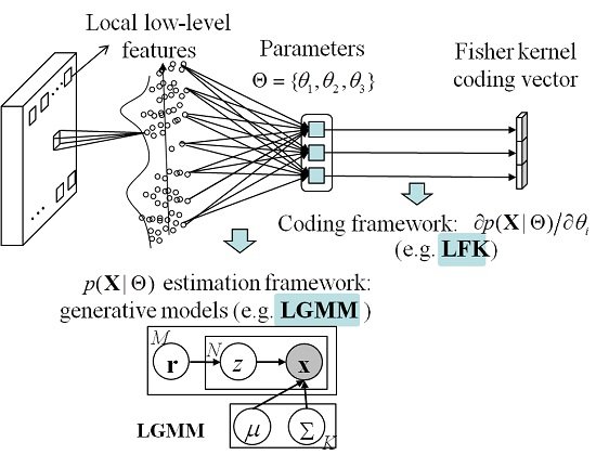
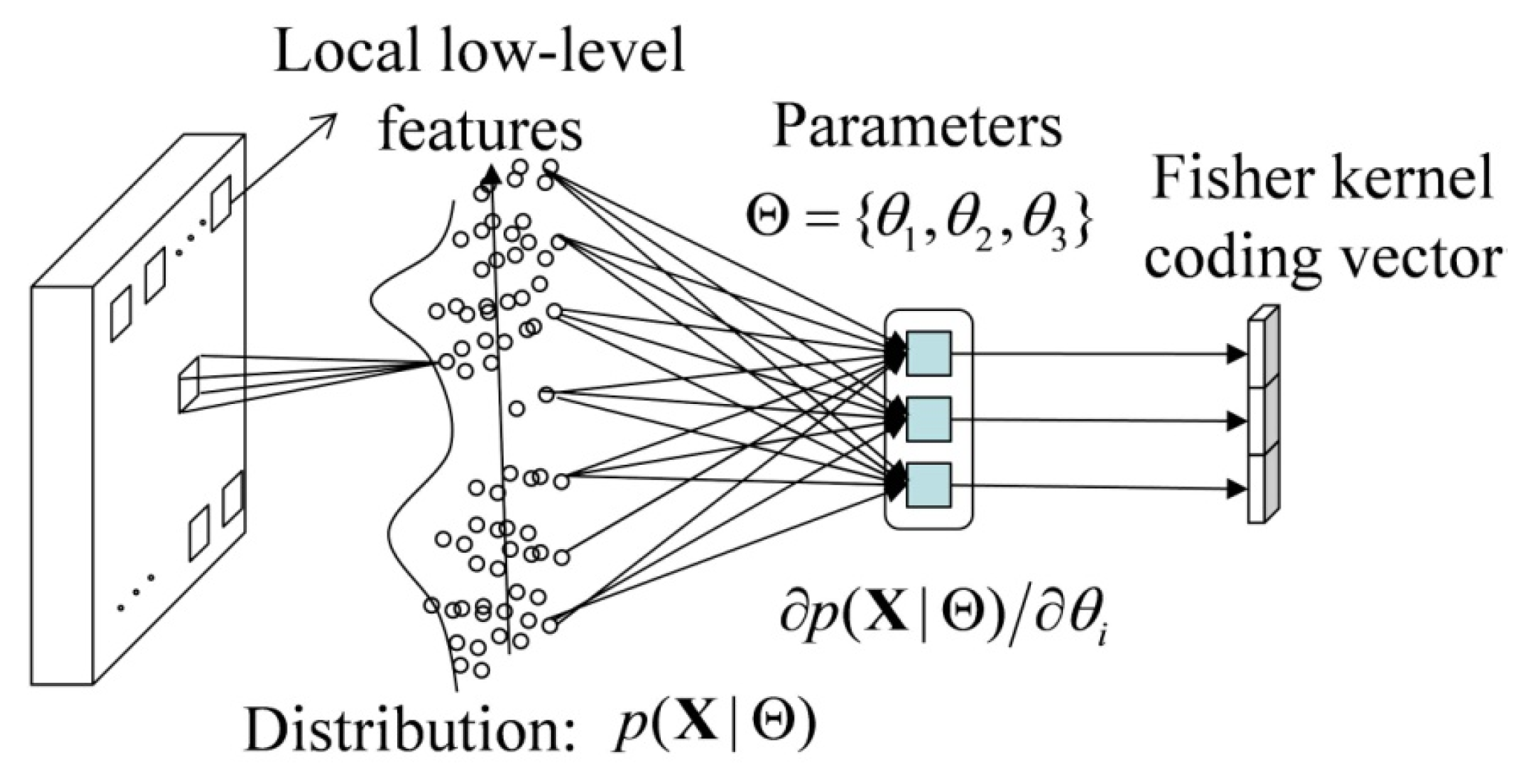
The Fisher kernel (FK) is a technique that combines the advantages of the generative and discriminative approaches by describing a signal with a gradient vector of its probability density function (PDF) with respect to the parameters of the PDF.
Figure 1 shows the FK coding framework that is used to obtain the representation of the HSR imagery.
We let
p be the PDF of the local low-level features. The set of local low-level features in a HSR image
can then be characterized by the gradient vector
, where
n is the number of patches in the image, and Θ is the set of parameters of the PDF. The gradient vector describes the magnitude and direction that the parameters are modified to fit the data. To normalize the gradient vector, the Fisher information matrix is recommended, which measures the amount of information that
X carries about the unknown Θ of the PDF, and can be written as:
The normalized gradient vector is then derived by:
Finally, the normalized gradient vector is used to represent the HSR image, and is classified by a discriminative classifier, such as SVM. Under this FK coding framework, the method of local low-level feature extraction, the probabilistic generative model, and the discriminative classifier can be changed according to the characteristics of these models and the HSR images.
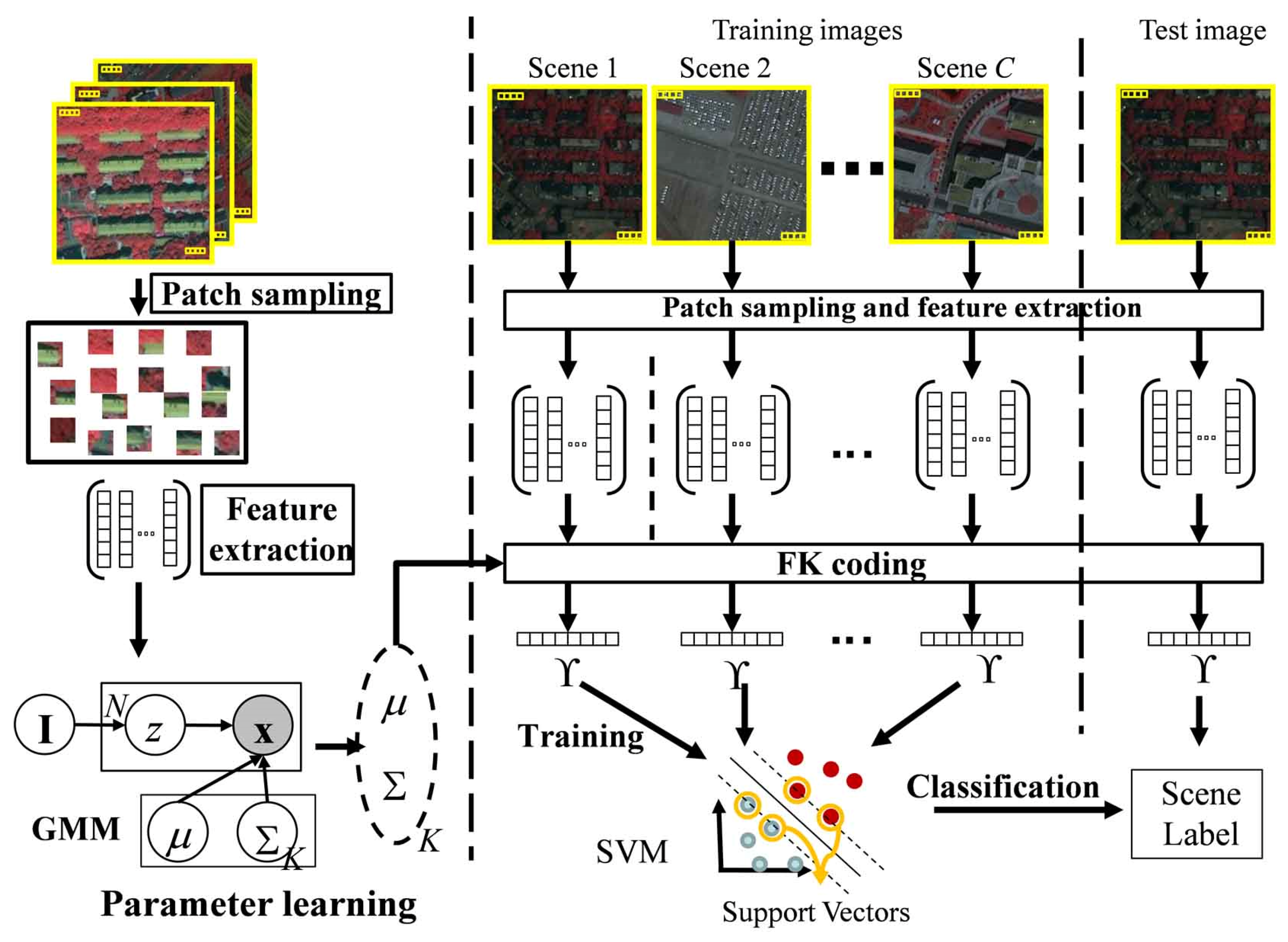
2.2. Scene Classification without the Consideration of the Spatial Information (FK-O)
In this part, FK-O is introduced to classify HSR scenes without the consideration of the spatial information. Under the FK coding framework, the GMM is employed as the probabilistic generative model to estimate the PDF of the low-level features. The FK coding is then performed to obtain the coding vectors to represent the HSR scenes. Finally, the coding vectors of the training images are used to train the discriminative classifier, SVM, which is used to classify the coding vectors of the test images (
Figure 2). The details are as follows.
2.2.1. Patch Sampling and Feature Extraction
For each scene image, the patches are evenly sampled from each region with a certain size and spacing (e.g., 8 × 8 pixels size and 4 pixels spacing), which are empirically selected to obtain a good scene classification performance. The local low-level features can then be extracted from the patches. To acquire the low-level features, there are many local descriptors, such as the descriptors based on the gray-level co-occurrence matrix [
24] and scale invariant feature transform (SIFT) [
25]. In this work, the mean/standard deviation statistics [
9] are used to extract the low-level features because of their simplicity and performance in HSR scene classification.
We let
x be the low-level features extracted from the patch, where
x can be obtained by computing the mean and standard deviation features of this patch with Equation (3). In Equation (3),
B is the number of spectral bands of the image,
n is the number of pixels in the patch, and
vp,b is the
b-th band value of the
p-th pixel in the patch
2.2.2. Fisher Kernel Coding and Scene Classification
To obtain a compact representation of the HSR scene, the FK coding method is introduced to code the low-level features into mid-level coding vectors, without losing too many details. Before the FK coding, the distribution of the low-level features should be estimated by the GMM. We let xj be the low-level feature of the j-th patch, and the sets of patches used to learn the parameters of the GMM can then be denoted by , where are the priors of the Gaussians, and Σ are the mean and covariance matrix of the k-th Gaussian component, D (D = 2B) is the dimension of the features, and K is the number of Gaussian components. For the FK coding, the covariance matrix Σ of each cluster is usually approximated by a diagonal matrix σ, where the diagonal elements are the variances of the features of the pixels in the cluster. We let d be the index of the components of the features, .
Given the low-level features
in an image, where
, and
n is the number of patches in the image, the image can then be described by the normalized gradient vector (Equation (4)) under the FK coding framework.
The FK coding vector with respect to
and
can be derived as shown in Equations (5) and (6), respectively, where the posterior probability
can be obtained by Equation (7),
The Fisher vector of an image can be written as
, where
and
. From Equations (5) and (6), it can be seen that the low-level features are coded by the gradient between the low-level features and the parameters of the Gaussian components, which infers that the coding vector can preserve the details of the low-level features as much as possible, compared to the traditional feature coding method based on the distance. In addition, in order to improve the performance, L
2-normalization and power normalization are recommended by Perronnin
et al. [
41]. After the FK coding, each image can be represented by an FK coding vector
.
Finally, the coding vectors of the training images are used to train an SVM classifier [
43], while the coding vector of the test image is classified by the trained SVM. During the training of the SVM classifier, the histogram intersection kernel (HIK) is adopted due to its performance in image classification [
44]. The HIK is defined as shown in Equation (8), where
q is the index of the component of the coding vector,
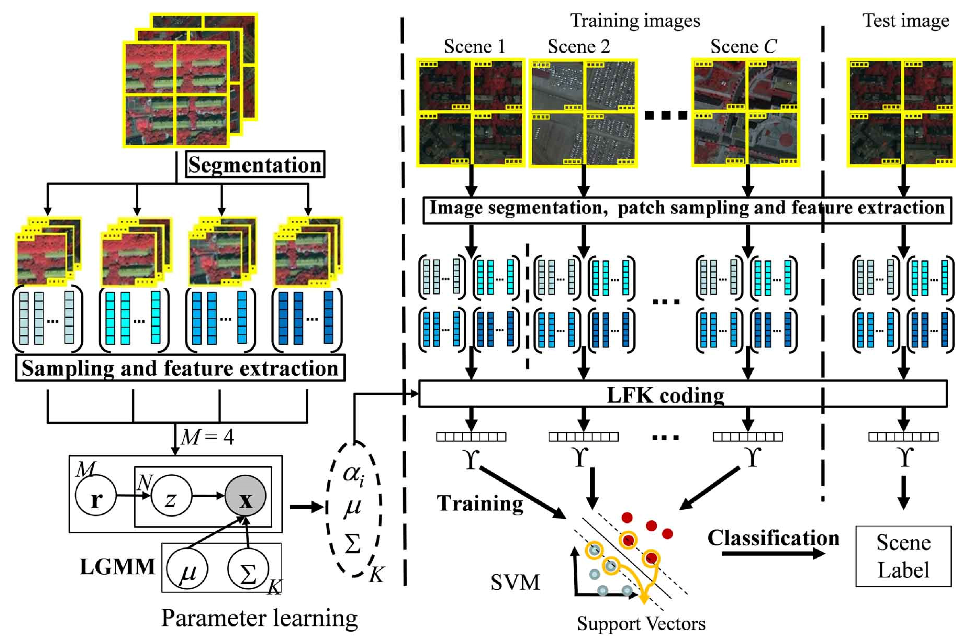
2.3. Scene Classification with the Consideration of the Spatial Information (FK-S)
In order to consider the spatial information, the scene classification method under the FK coding framework for HSR scenes, FK-S, is proposed in this part. The procedure of the proposed method is shown in
Figure 3.
Instead of the GMM, FK-S uses the LGMM to estimate the distribution of the low-level features by considering the difference between different regions of the HSR scenes, while LFK is developed to code the HSR images to adapt to the change brought about by the change of distribution estimation method. The details of FK-S are described in the following parts.
2.3.1. Image Segmentation, Patch Sampling, and Feature Extraction
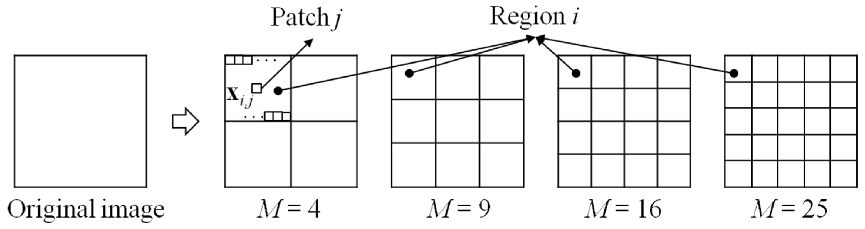
For each scene image, chessboard segmentation is used to split the whole image into multiple regions, while the patches are evenly sampled from each region with a certain size and spacing. The local low-level features can then be extracted from the patches.
Figure 4 shows the multiple regions of an image produced by chessboard segmentation with different numbers of regions
M, where
i is the index of the regions,
j is the index of the patches, and
xi,j is the low-level feature extracted from the
j-th patch in the
i-th region.
As in FK-O, FK-S also employs the mean/standard deviation statistics to extract the low-level features (Equation (3)). We let xi,j,d be the d-th component of xi,j, and , where D is the dimension of the low-level features. All the regions of the images can then be denoted as , where M is the number of regions, is the set of low-level features in the i-th region, and ni is the number of patches in the i-th region.
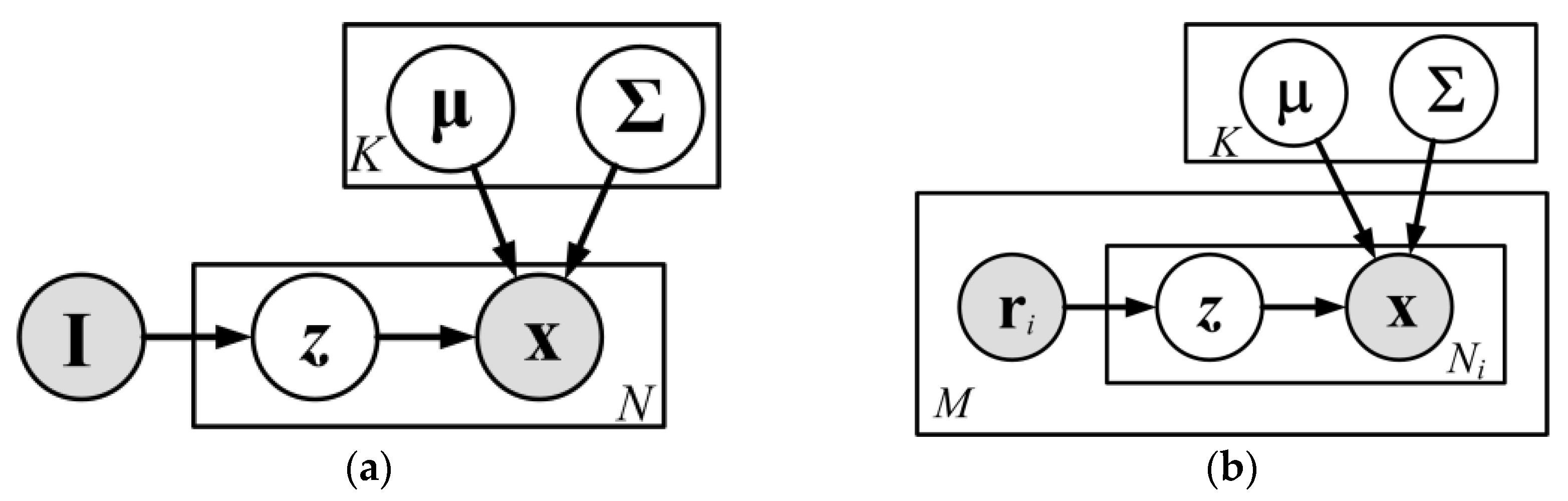
2.3.2. Learning the Parameters of the Local Gaussian Mixture Model (LGMM)
Considering that the traditional GMM (
Figure 5a) generates all the features
x in the whole scope of the images from Gaussians with the same priors
P(
z|
I) (also known as mixing weights), which ignores the spatial arrangement of the HSR images during the estimation of the distribution of the low-level features, the LGMM (
Figure 5b) is used to learn the distribution of the low-level features, where the features
x in the different regions are generated from Gaussians with different priors
. In particular, for the
i-th region
ri, the identities of the Gaussians
z are generated from the priors
P(
z|
ri), and the features
x in this region can then be extracted from the Gaussians identified by the corresponding
z. Due to the different treatment of different regions, the LGMM is able to estimate different sets of priors of Gaussians for different regions
, which reflects the different distributions of low-level features in the different regions. Therefore, the distribution of the low-level features estimated by the LGMM can take into account the spatial arrangement of the low-level features.
We let z
i,j be the latent value of the low-level feature
xi,j in
ri, and the probability of pixel
being drawn from the
k-th Gaussian (
) is described in Equation (9), where
and
are the mean vector and the covariance matrix of the
k-th Gaussian, respectively,
In order to learn the parameters of the distribution of the low-level features for the HSR scenes, a number of images are randomly selected from the HSR image dataset, and should be divided into
M regions by chessboard segmentation (
Figure 3). All the low-level features of patches in the same region of all the selected images are collected and form a new set of features
, where
,
, and
nl,i is the number of patches in the
i-th region of the
l-th selected image. Assuming that all the local low-level features are independent, the log-likelihood of all the features can be formulated by Equation (10), where
. The log-likelihood of all the features is then parameterized by
.
The expectation-maximization (EM) algorithm is employed to estimate the parameters of the LGMM, as in the GMM. The EM algorithm begins with an initial estimate and repeats the following two steps:
E-step. Compute the expected value
of the log-likelihood function with respect to the conditional distribution
, according to Equation (11).
In Equation (11)
, can be calculated by Equation (12),
M-step. Maximize
with the constraint that
to obtain the update equation of parameters
. To solve this problem, Lagrange multipliers
are introduced into the objective function
. The new objective function
can then be rewritten as:
To obtain the updated equation of
,
, and
, the objective functions are obtained by isolating the terms with
,
, and
, respectively, and can be written as:
By maximizing the objective functions, the updated equations of
,
, and
can be obtained as shown in Equations (17)–(19), respectively:
The EM algorithm is terminated when the last two values of the log-likelihood are close enough (below some preset convergence threshold) or the number of iterations reaches the preset number. Similarly, assuming that the components of the feature vectors are independent, the covariance matrix
of each Gaussian can be replaced with a diagonal matrix
. Equations (9) and (19) can then be rewritten as Equations (20) and (21), respectively, where
,
The M sets of features are then used to learn the parameters by the use of the LGMM.
2.3.3. Local Fisher Kernel (LFK) Coding and Scene Classification
To incorporate the spatial information contained in the parameters obtained by the LGMM, an LFK coding method is proposed under the FK coding framework.
Given the low-level features
in an image, the LFK coding vector of the image can then be described by Equation (22) under the FK coding framework, where
ni is the number of patches in the
i-th region of the image,
The LFK coding vector with respect to
,
, and
can be derived as shown in Equations (23)–(25), respectively, where the posterior probability
can be obtained by Equation (12) with the parameters
,
Finally, the LFK coding vector of an image can be written as , where , , and . It is worth noting that the LFK coding vector with respect to the priors contains the spatial information obtained by the LGMM, and the number of components of M(K−1) should be kept at less than 50% of the dimension of the LFK coding vector, 2KD+M(K−1), to ensure that the spatial information is less important than the low-level feature information in the coding vector. Therefore, the number of regions M should be less than 2KD/(K−1)≈2D. In addition, when M is a small number, the importance of the spatial information decreases, and we recommend that M should be set as larger than 1. For example, when the number of bands of the images B = 3, then D = 2B = 6, and 1 < M < 2D = 12. Between M = 4 and M = 9, we recommend M = 9, because it can explore more spatial information for the HSR scene images.
As in FK-O, L2-normalization and power normalization are recommended to improve the performance of FK-S. After the LFK coding, each image can be represented by an LFK coding vector . Finally, the coding vectors of the training images are used to train an SVM classifier with HIK, while the coding vector of the test image is classified by the trained SVM.
Both FK-O and FK-S are developed under the FK coding framework, where the low-level features are coded by the gradient between the low-level features and the parameters of the Gaussian components, which leads to the ability to preserve more of the details of the low-level features than the traditional feature coding method based on the distance.
4. Results and Accuracies
The FK-O method obtained the highest classification accuracies when the number of Gaussians
K was set to 128, 64, and 32 for the UCM dataset, the Google dataset, and the Wuhan IKONOS dataset, respectively, while the FK-S method obtained the best performance when
K was set to 128, 128, and 32 for the UCM dataset, the Google dataset, and the Wuhan IKONOS dataset, respectively. For all the datasets, when the number of regions
M was set to 9, FK-S acquired the best accuracy. The classification accuracies of the different methods for the three image datasets are reported in
Table 1. Here, it can be seen that the feature coding methods under the FK coding framework, namely FK-O and FK-S, acquired accuracies of 91.38 ± 1.54(%) and 91.63 ± 1.49(%) for the UCM dataset, 90.16 ± 0.82(%) and 90.40 ± 0.84(%) for the Google dataset, and 89.67 ± 4.19(%) and 90.71 ± 4.41(%) for the Wuhan IKONOS dataset, respectively.
(1) Comparison between the feature coding methods under the FK coding framework and the traditional methods based on the BOVW. When compared to the traditional BOVW method, scene classification based on FK-O and FK-S improved the classification accuracy by about 19% for the UCM dataset and about 9%–10% for the Google dataset and the Wuhan IKONOS dataset. In contrast to the SPM-MeanStd method, FK-O and FK-S increased the accuracy by about 6%, 4%, and 2% for the UCM dataset, the Google dataset, and the Wuhan IKONOS dataset, respectively. Compared to the LDA and P-LDA methods, FK-O and FK-S improved the accuracy by more than 9%, 8%, and 5% for the UCM dataset, the Google dataset, and the Wuhan IKONOS dataset, respectively.
(2) Comparison between before and after considering the spatial information. For all the datasets, the FK-S scene classification method obtained slightly higher classification accuracies than the FK-O scene classification method, which suggests that considering the spatial information during the parameter learning and coding can improve the classification performance.
(3) Comparison between the linear kernel and HIK kernel of SVM. The FK-O (FK-S) scene classification method with HIK kernel increased the accuracy by about 2%, 2%, and 10% when compared to the FK-Linear (LFK-Linear) classification method with linear kernel for the UCM dataset, the Google dataset, and the Wuhan IKONOS dataset, respectively.
(4) Comparison of the codebook size. For FK-O and FK-S, the size of the codebook is the number of Gaussian components
K. The sizes of BOVW, FK-O, and FK-S codebooks corresponding to the accuracies in
Table 1 are recorded in
Table 2, where the codebook sizes of FK-O are 128, 64, and 32, while the codebook sizes of FK-S are 128, 128, and 32 for the UCM dataset, the Google dataset, and the Wuhan IKONOS dataset, respectively. The codebook size of BOVW is 1000 for all the datasets. By the use of a PC with a 2.5 GHz Intel Core i5-3210M processor, the cost times of the different methods are reported in
Table 2, which infers that the cost times of FK-O and FK-S are less than those of BOVW.
Table 2 also indicates that the cost times of FK-S are greater than those of FK-O. This evidence infers that scene classification under the FK coding framework can reduce the size of the codebook and the computational cost, to obtain a more compact representation of the scenes.
(5) Comparison with the state-of-the-art. The published classification accuracies of different methods for the UCM dataset are shown in
Table 3. Here, it can be seen that the FK-O and FK-S scene classification methods acquired a very competitive accuracy when compared to the state-of-the-art.
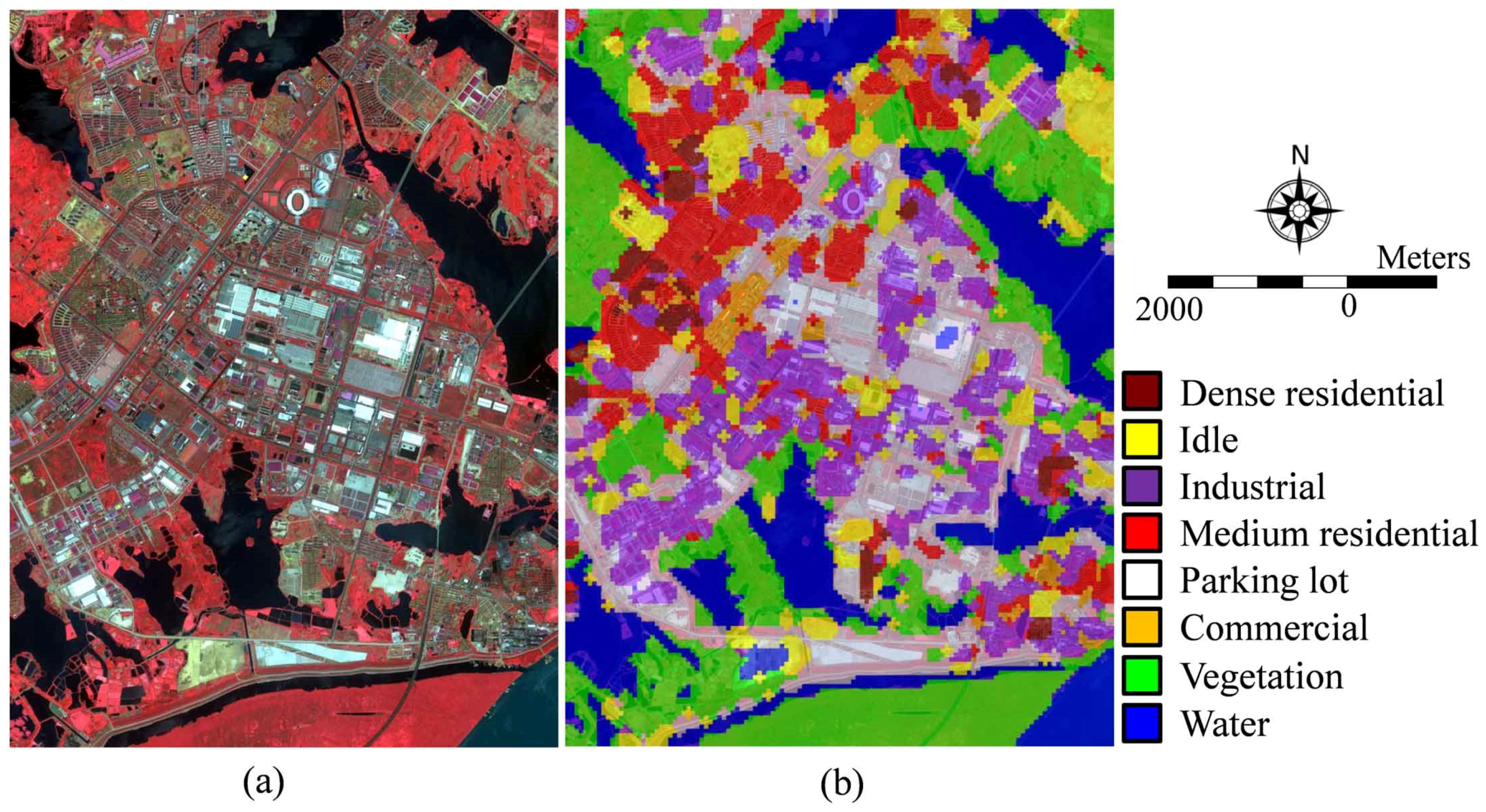
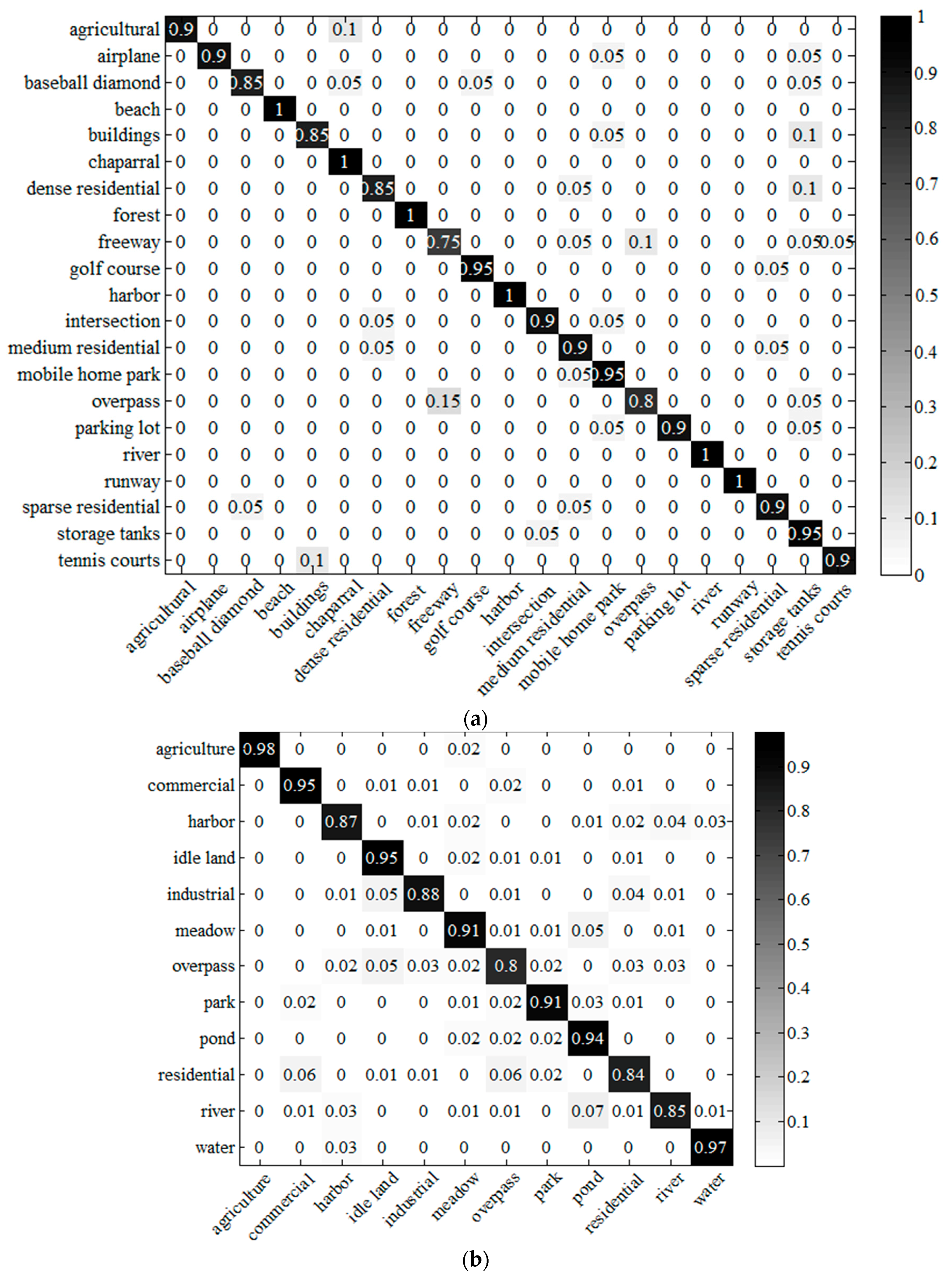
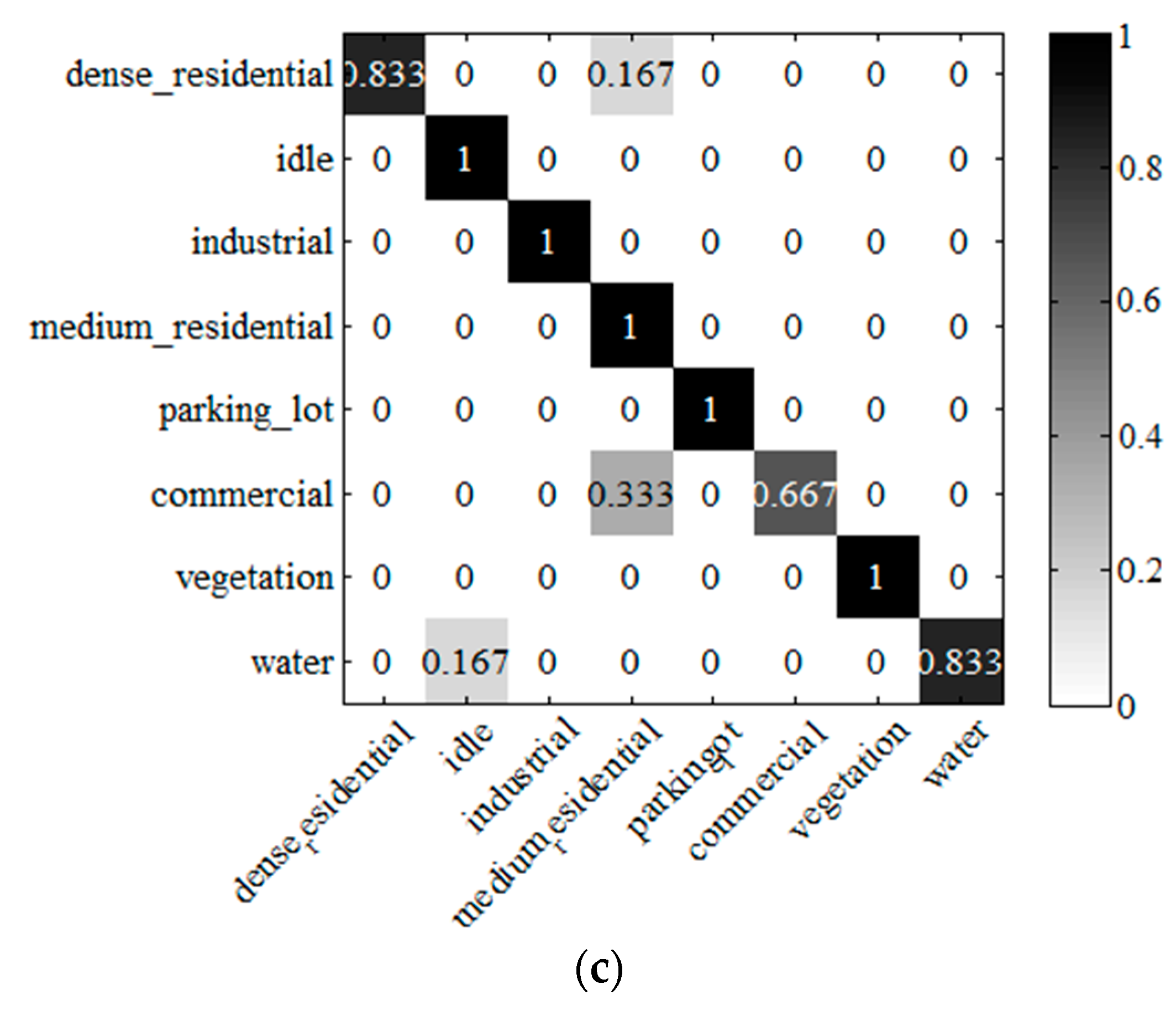
(6) Evaluation of the performance of the scene classification and annotation methods developed under the FK coding framework for each scene class. Taking FK-S as an example, the classification confusion matrices of the three datasets are shown in
Figure 11, and the annotated image for the large Wuhan IKONOS image is shown in
Figure 9b.
From the confusion matrix of the UCM dataset (
Figure 11a), it can be seen that the accuracies of all the scenes, except for the freeway class, are more than 80%, and the relatively low accuracy of the freeway scene is mainly caused by the confusion with the overpass scene. In addition, the confusion levels of the following pairs of scenes exceed 10%: agricultural/chaparral, buildings/storage tanks, and dense residential/storage tanks. For the Google dataset (
Figure 11b), the accuracies of all the scenes are more than 80%, and the main confusion occurs in the pairs of scenes of residential/commercial, river/pond, and residential/overpass. For the Wuhan IKONOS dataset (
Figure 11c), the accuracies of all the scenes are higher than 80%, except for the commercial scene, and the main confusion occurs between the commercial scene and the medium residential scene. One of the main reasons for the confusion is that some images in these pairs of scenes are very similar in spectral value, and the mean and standard deviation statistics of the spectral values have a limited ability to describe the difference. Therefore, finding a proper feature extractor for the HSR scene classification, or combining different feature extractors with different characteristics, are potential ways to improve the performance. For the annotation experiment, although there is some confusion between industrial, parking lot, commercial, dense residential, and medium residential, the annotated large image is still satisfactory, based on our remote sensing image analysis expertise.
5. Discussion
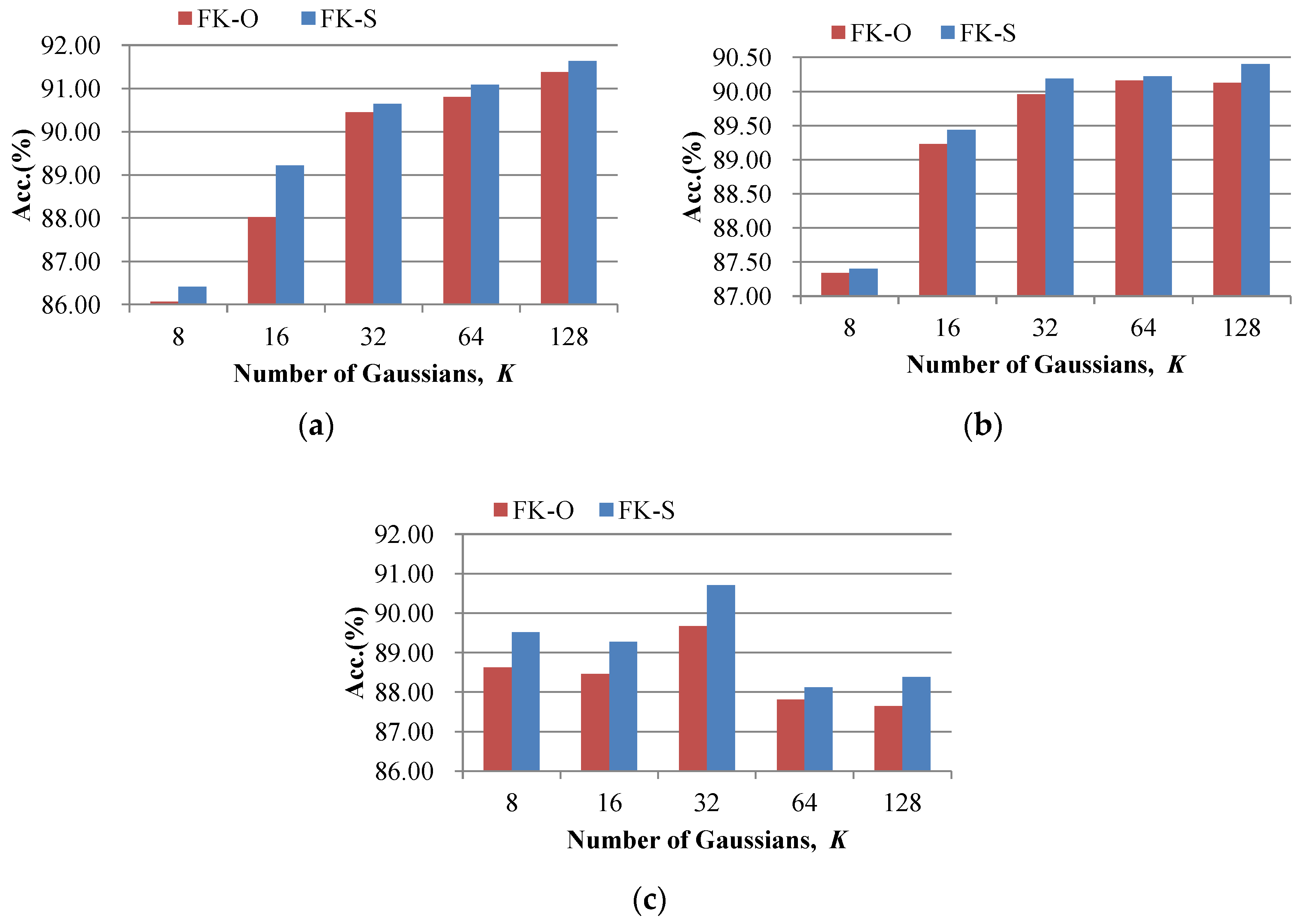
In the FK-O and FK-S scene classification methods, the number of Gaussians
K is an important parameter, which is discussed in this section (
Figure 12). In addition, the effect of the number of regions
M for the FK-S scene classification method is also analyzed (
Figure 13).
(1) The effect of the number of Gaussians
K. In the experiments,
K was varied between 8, 16, 32, 64, and 128. The accuracies of the FK-O and FK-S scene classification methods with different
K values are shown in
Figure 12, where the number of regions was set to nine for FK-S. From
Figure 12, it can be seen that the classification accuracies of the FK-O and FK-S scene classification methods increased rapidly with the increase in
K from eight to 32, but the magnitude of the increase was small when
K was increased from 32 to 128 for the UCM dataset and the Google dataset. For the Wuhan IKONOS dataset, the best performances for the FK-O and FK-S scene classification methods were acquired when
K was set to 32, and a smaller or bigger
K caused a decrease in the classification accuracy. This is because a small codebook lacks the descriptive ability for the low-level features, while a large codebook contains redundant visual words, which leads to the high dimension of the coding vector (2
KD+
M(
K−1)) and high correlation between the components. When compared to the FK-O scene classification method, the FK-S scene classification method obtained higher accuracies.
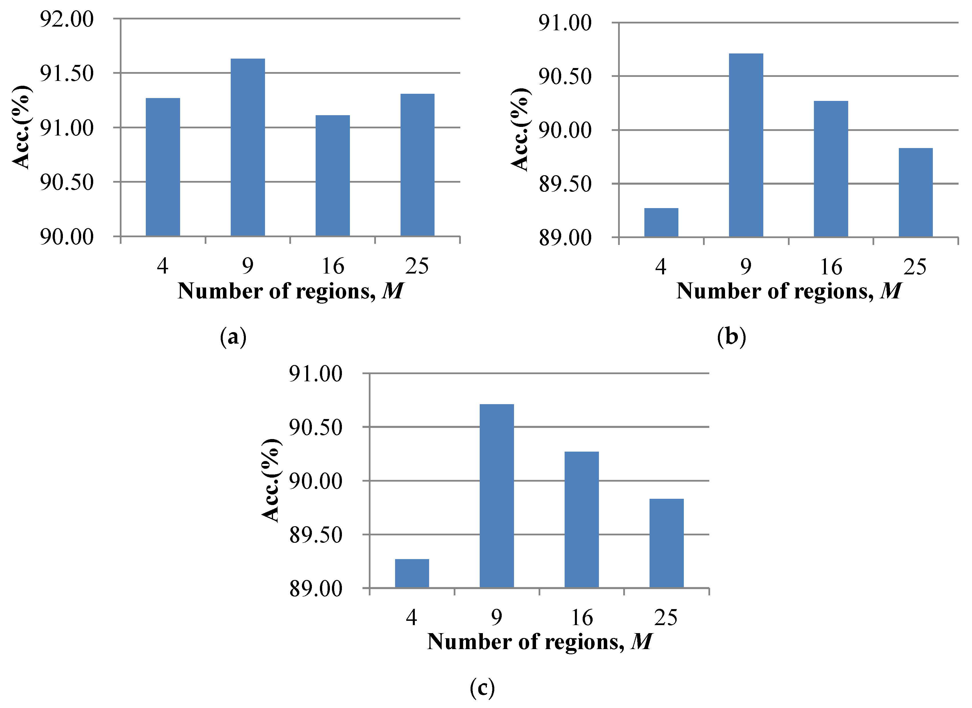
(2) The effect of the number of regions
M for the FK-S scene classification method. In the experiments,
M was varied between 4, 9, 16, and 25. The accuracies of the FK-O and FK-S scene classification methods with different
M values are shown in
Figure 13. In
Figure 13, the best accuracies for the FK-S scene classification method were acquired when
M was set to nine for all three datasets. A larger number of regions, e.g.,
M = 16, led to a decrease in the classification accuracy, because there were too many components in the LFK coding vector describing the spatial information. Meanwhile, a smaller number of regions led to a smaller number of spatial components, which resulted in less use of the spatial information during the scene classification.
6. Conclusions
In order to bridge the semantic gap between the low-level features and high-level semantic concepts for high spatial resolution (HSR) imagery, we introduce a compact representation for HSR scenes under the Fisher kernel (FK) coding framework by coding the low-level features with a gradient vector instead of the count statistics in the BOVW model. Meanwhile, a scene classification method is proposed under the FK coding framework to incorporate the spatial information, where the local Gaussian mixture model (LGMM) is used to consider the spatial arrangement by estimating the different sets of priors of the Gaussians for the low-level features in different regions, and a local FK (LFK) coding method is developed to deliver the spatial information into the coding vectors. The scene classification methods developed under the FK coding framework, with and without the incorporation of the spatial information, are called FK-S and FK-O, respectively. The experimental results with the UCM dataset, a Google dataset, and an IKONOS dataset infer that the scene classification methods developed under the FK coding framework are able to generate a compact representation for the HSR scenes, and can decrease the size of the codebook. In addition, the experimental results show that the scene classification method incorporating the spatial information, FK-S, can acquire a slightly better performance than the scene classification method that does not consider the spatial information, FK-O. When compared to the published accuracies of the state-of-the art for the UCM dataset, the scene classification methods under the FK coding framework can obtain a very competitive accuracy.


