Article

A Comparative Study of Cross-Product NDVI Dynamics in the Kilimanjaro Region—A Matter of Sensor, Degradation Calibration, and Significance

Environmental Informatics, Faculty of Geography, Philipps-Universität Marburg, Deutschhausstr. 12, 35032 Marburg, Germany
*
Author to whom correspondence should be addressed.
Submission received: 7 December 2015 / Revised: 20 January 2016 / Accepted: 14 February 2016 / Published: 19 February 2016
(This article belongs to the Special Issue Multi-Sensor and Multi-Data Integration in Remote Sensing)

Abstract

:
While satellite-based monitoring of vegetation activity at the earth’s surface is of vital importance for many eco-climatological applications, the degree of agreement among certain sensors and products providing estimates of the Normalized Difference Vegetation Index (NDVI) has been found to vary considerably. In order to assess the extent of such differences in highly heterogeneous terrain, we analyze and compare intra-annual seasonal fluctuations and long-term monotonic trends (2003–2012) in the Kilimanjaro region, Tanzania. The considered NDVI datasets include the Moderate Resolution Imaging Spectroradiometer (MODIS) products from Terra and Aqua, Collections 5 and 6, and the 3rd Generation Global Inventory Modeling and Mapping Studies (GIMMS) product. The degree of agreement in seasonal fluctuations is assessed by calculating a pairwise Index of Association (IOAs), whereas long-term trends are derived from the trend-free pre-whitened Mann–Kendall test. On the seasonal scale, the two Terra-MODIS products (and, accordingly, the two Aqua-MODIS products) are best associated with each other, indicating that the seasonal signal remained largely unaffected by the new Collection 6 calibration approach. On the long-term scale, we find that the negative impacts of band ageing on Terra-MODIS NDVI have been accounted for in Collection 6, which now distinctly outweighs Aqua-MODIS in terms of greening trends. GIMMS NDVI, by contrast, fails to capture small-scale seasonal and trend patterns that are characteristic for the highly fragmented landscape which is likely owing to the coarse spatial resolution. As a short digression, we also demonstrate that the amount of false discoveries in the determined trend fraction is distinctly higher for p < 0.05 ( 52.6 % ) than for p < 0.001 ( 2.2 % ) which should point the way for any future studies focusing on the reliable deduction of long-term monotonic trends.

Graphical Abstract

1. Introduction

The Normalized Difference Vegetation Index (NDVI) [1] is widely applied in the fields of eco-climatological research to deduce seasonal and long-term vegetation dynamics from remotely sensed imagery. Despite its outstanding scientific value to monitor vegetation greenness at the earth’s surface, it became evident that analyzing data from different sensor systems resulted in considerably deviating signals which was attributed to quite a variety of factors. In this context, Alcaraz-Segura et al. [2] compared 8-km Advanced Very High Resolution Radiometer (AVHRR) Global Inventory Modeling and Mapping Studies (GIMMS) NDVI [3] over North America against a 1-km product provided by the Canadian Centre for Remote Sensing (CCRS) [4]. Based on the seasonal Mann–Kendall trend test [5] calculated from the mean growing season NDVI (1984–2006) and with a particular focus on post-fire vegetation recovery, the authors demonstrated that GIMMS widely documented “browning” (in terms of a declining trend) as opposed to unexceptional “greening” (in terms of an increasing trend) observable from the CCRS dataset. The observed differences were attributed to an inappropriate correction of the satellite drift and to the rather coarse spatial and temporal resolution of the half-monthly GIMMS dataset as compared to the 10-day CCRS product. More recently, Fensholt and Proud [6] compared global vegetation trends (2000–2010) derived from GIMMS and the Moderate Resolution Imaging Spectroradiometer (MODIS) aboard the Terra satellite, Collection 5 (NDVITerra-C5). While the datasets were in generally good agreement, which particularly applies to regions with a clear phenological cycle, considerable discrepancies became evident (i) over evergreen equatorial forests with a constantly high NDVI signal; (ii) in sparsely vegetated high-latitude regions; and (iii) in arid areas with low photosynthesis rates. By contrast, Guay et al. [7] only recently reported that trends (2002–2007) deduced from AVHRR GIMMS and combined Terra/Aqua-MODIS observations over high northern latitudes (above 50 °N) agreed reasonably well, thus seemingly contradicting the above point (ii). However, their findings need to be interpreted more cautiously due to the shorter temporal coverage as compared to the study by Fensholt and Proud [6].
Complementing such multi-sensor approaches, considerable differences were found to also occur among sensors of the same type. Wang et al. [8], for instance, demonstrated that NDVITerra-C5 revealed about three times more browning over North America as compared to the Collection 5 product derived from Aqua-MODIS (NDVIAqua-C5; 2002–2010). Due to identical sensor characteristics in terms of temporal (16-day) and spatial (250-m) resolution, the authors concluded that Terra-MODIS bands 1 (red, 620–670 nm) and 2 (near infra-red, 841–876 nm) markedly suffered from sensor degradation which resulted in a higher portion of browning. A more comprehensive overview of the particular impacts of band ageing on Terra-MODIS and, to a lesser extent, on Aqua-MODIS products has recently been provided by Lyapustin et al. [9]. The authors emphasized that the effects of sensor degradation generally decrease with wavelength, rendering the impacts on the calculation of Terra-MODIS NDVI particularly severe, not least because of the insufficient degradation calibration. At the same time, they pointed out that such differences could be expected to disappear with the improved calibration approach used to create the recently released Collection 6 of the MODIS “Vegetation Index” product series [10].
In the scope of a comprehensive study of regional-scale vegetation dynamics in the Kilimanjaro region, Tanzania [11], we adopt and extend some of the depicted approaches to pre-analyze and evaluate possible differences among a selection of NDVI products covering the period from 2003 to 2012. Included are the 250-m and 0.05-degree MODIS products originating from Collection 5 (NDVITerra-C5 and NDVIAqua-C5) and Collection 6 (NDVITerra-C6 and NDVIAqua-C6). Due to its long-term temporal coverage and the broad range of applications resulting therefrom, this initial selection is complemented by the recently updated “3rd Generation GIMMS NDVI” dataset (NDVI3g) [12]. A particular focus is thereby put on the cross-product comparison of seasonal (intra-annual) and trend (inter-annual) patterns, while the underlying natural and anthropogenic driving factors receive only little attention. The agreement on the seasonal scale is assessed using a simple Index of Association (IOAs), whereas long-term trends are captured using the trend-free pre-whitened (TFPW) Mann–Kendall test. With regard to the latter, we also present a short digression on the effects of the chosen significance level (p) on the number of identified trends and the amount of false alarms associated therewith.

2. Experimental Section

2.1. Study Area

The Kilimanjaro area is located in the north-eastern part of Tanzania close to the Kenyan border and is limited to a geographic extent from 36.9 to 37.8 °E and 2.7 to 3.5 °S within the scope of this study. The region is characterized by a highly dynamic relief with elevations rising from the savanna plains at around 700 meters above sea level (in the following simply referred to as “m”) to the glaciated areas encircling Kibo summit (5895 m). Considering the climatic gradient that such a broad elevation profile entails – Appelhans et al. [13] recently reported mean annual air temperatures of more than 25 °C in the savanna plains and less than - 5 °C on the summit—the horizontal distance between prevailing land covers is relatively short when moving upward along the mountainside [14]. The region’s equatorial daytime climate [15] is shaped by a bimodal distribution of annual rainfall [16] that can roughly be subdivided into “long rains” (March to May) and “short rains” (around November) according to the passing of the intertropical convergence zone. The southern slopes typically receive more than half of the annual rainfall during the long rains as a consequence of moist south-easterly winds [17], whereas prolonged short rains dominate in north-east-facing locations. Overall, accumulated annual rainfall totals more than 2500 mm in the southern montane forest belt, while the northern mountainside receives hardly more than 1000 mm at maximum [18].
The regional vegetation has only recently been summarized by Maeda and Hurskainen [19] based, amongst others, on the exhaustive studies by Hemp [15,18], and the reader is kindly referred to this list of profound works for further information. Briefly, the mountain’s distinct vegetation zonation—also referred to as “bioclimatic belts” in Hemp [15] (p. 1014)—starts with a broadly cultivated, colline savanna zone (700 to 1000 m) that underlies a clearcut phenological cycle tailored to the bimodal annual rainfall distribution [11]. The savanna zone is followed by a densely populated, intensely managed submontane zone (1000 to 1800 m) which mainly comprises coffee and banana plantations and expands until the lower boundary of Kilimanjaro National Park (~1800 m). A densely vegetated, evergreen montane forest belt and the subalpine zone (~2800 m), the latter being dominated by Erica forest (E. excelsa) that gradually changes into Erica bush (E. arborea, E. trimera) and Helichrysum cushion, follow in uphill direction. Starting from 4500 m upward, only little vegetation is left. Note that in contrast to the savanna plains and the densely vegetated foothills, a clear phenological cycle is hardly observable inside the forest and in the upper-mountain regions.

2.2. Satellite Data

2.2.1. MODIS NDVI

The Terra-MODIS (MOD13Q1) and Aqua-MODIS (MYD13Q1) “Vegetation Index” products [20] originating from Collections 5 [21] and 6 [10] are downloaded from the Land Processes Distributed Active Archive Center [22] and come in a spatial resolution of 250 m (MODIS Sinusoidal projection [23]). Data reprocessing in preparation for the release of Collection 6 was initialized in February 2015 [24] in order to address, among others, calibration trends resulting from Terra-MODIS sensor degradation. For further information, the reader is kindly referred to Lyapustin et al. [9] who provide a summary of the main motives and algorithm changes underlying the release of Collection 6.
For both product versions, data processing includes the removal of all pixels flagged “cloudy” in the associated “pixel reliability summary” layer. Further cloud remnants are captured based on quantile thresholds applied to the residuals of each pixel time series as implemented by Hyndman [25] in the R forecast package (and function tsoutliers therein) followed by the application of a three-by-three focal mask around each pixel discarded so far. The introduced gaps are subsequently refilled using the so-called Whittaker smoother (WS). Atzberger and Eilers [26] proposed this algorithm to smooth time series observations of vegetation indices by removing noise originating from undetected clouds, thus downweighting low—and possibly distorted—values in favor of high values assumed to represent the “true” vegetation signal. Finally, the 16-day images are aggregated to monthly maximum value composites (MVC; n = 120 layers) based on the accompanying “composite day of the year” layer and converted to EPSG:4326 (WGS 84/Latlong) using the nearest neighbor method.
When in combination with NDVI3g, we use the monthly MODIS 0.05-degree geographic climate modeling grids (CMG; MOD13C2 and MYD13C2) instead of the 250-m products. Here, data processing includes the rejection of all “cloudy” or “estimated” pixel values [21] which are subsequently refilled via the WS. The monthly layers are spatially aggregated to the regular NDVI3g grid by calculating the area-weighted sum of all 0.05-degree MODIS CMG grid cells intersecting a particular 1/12-degree GIMMS grid cell.
Note that all MODIS pixels with a long-term mean value of the NDVI smaller than 0.15 are treated as non-vegetated surfaces (e.g., suggested by Wittich and Hansing [27]) and are hence not considered during seasonal (Section 2.3.1) and trend analysis (Section 2.3.2). This limitation is owing to the fact that low NDVI signals over sparsely and non-vegetated surfaces, particularly bare ground, snow and ice, cannot be unambiguously assigned to actual vegetation or the influence of atmospheric variations and sensor characteristics [28].

2.2.2. AVHRR GIMMS NDVI3g

The NDVI3g product [12] is downloaded from the Ecological Forecasting Lab at NASA Ames Research Center [29] and comes in a spatial resolution of 1/12 degree (EPSG:4326; in the following also referred to as “8-km”). According to the accompanying quality flags [12, Appendix B], the majority of pixel values under consideration are of good quality (flagged “1”, 85.3%). Artificial values derived either from spline interpolation (flagged “3”, 12.5%) or the average seasonal profile (flagged “5”, 2.2%) contribute only to a minor degree, but are nonetheless considered as unreliable [6], and hence discarded [30]. Similar to the acquired MODIS products (Section 2.2.1), the half-monthly images subsequently undergo Whittaker smoothing (including gap-filling) and are aggregated to monthly MVC ( n = 120 layers) in order to ensure temporal overlap with the created MODIS MVC layers. In contrast to the latter, there are no NDVI3g grid cells with a long-term mean value falling below 0.15 , and hence no rejections in preparation for seasonal and trend analysis are required. Note that all GIMMS-related processing steps including data download, file format conversion, quality control, monthly aggregation and subsequent application of the TFPW Mann–Kendall test are included in the R gimms package which has been specifically developed for this study and is publicly available online [31].

2.3. Summary of Applied Methods

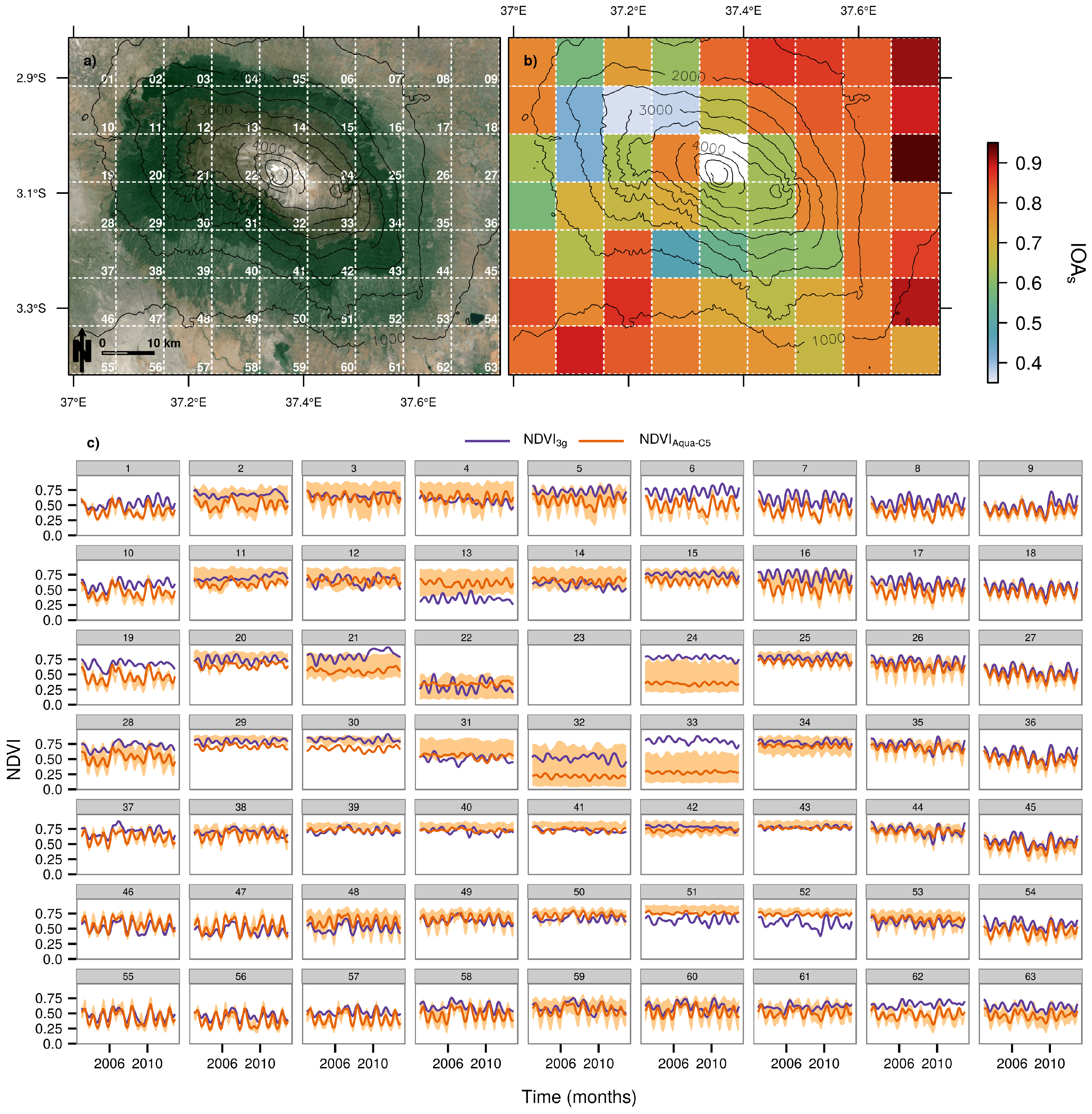
2.3.1. Index of Association

We adopt the algorithm implementation of a simple IOAs proposed by Matloff [32] to account for cross-product (dis-)similarities in seasonal fluctuations. It is calculated from
IOA s = 1 n × i = 2 n 1 , if s i g n ( x i - x i - 1 ) = s i g n ( y i - y i - 1 ) , 0 , if s i g n ( x i - x i - 1 ) s i g n ( y i - y i - 1 ) ,
where x and y are two series of observations with uniform length n. s i g n ( x i - x i - 1 ) is equal to 1, 0, or –1 depending on whether the value at the x i -th position is bigger, equal to, or smaller than the value at the x i - 1 th position (the same applies to the values of y). In a nutshell, IOAs spans a range from 0 to 1 where the former (latter) indicates that x and y never (always) increase or decrease in parallel, thus determining the degree of agreement between pairs of datasets on a monthly basis.

2.3.2. Mann–Kendall Trend Test

In order to prepare the individual datasets for long-term trend deduction, we create monthly NDVI anomalies by subtracting the long-term monthly means from the corresponding MVC layers [33]. This processing step ensures that seasonal fluctuations, which primarily result from the bimodal annual rainfall distribution, do not weaken [34] or even obscure the actual trend signal.
We then apply pre-whitening using the method described in Yue et al. [35] to remove lag-1 autocorrelation from the monthly anomalies. Serial correlation is generally recognized to influence trends in autocorrelated time series, including NDVI [36], which typically results in a higher portion of observed trends. To account for such overestimations, the algorithm uses the Theil–Sen approach [37] to determine whether the linear slope of a given time series significantly differs from zero. If the latter applies, this assumed trend signal is removed (“detrending”) from the initial data and the first-order autocorrelation is calculated and removed from the resulting residuals [38]. Finally, the cleansed residuals and the trend component are blended back together in order to obtain a pre-whitened version of the initial time series. Due to the application of detrending prior to removing the serial autocorrelation, the procedure is also referred to as trend-free pre-whitening [35].
The prepared data is finally used to compute Mann–Kendall trends [39] on a pixel basis from January 2003 until December 2012. The non-parametric test is based on the rank correlation coefficient (τ; herein after referred to as Kendall’s τ) firstly described by Kendall [40]. In contrast to the initial algorithm which requires two observation series as input variables, the modified version proposed by Mann [39] requires an observation series y and an accompanying time vector x (of length n) to deduce monotonous trends over time [41]. Kendall’s τ as a measure for trend direction and strength is calculated from
τ = S n ( n - 1 ) / 2 .
S is the so-called Kendall score [42] and derives from
S = i = 2 n 1 , if y i - y i - 1 > 0 , 0 , if y i - y i - 1 = 0 , - 1 , if y i - y i - 1 < 0 ,
where the term y i - y i - 1 equals 1, 0, or - 1 depending on whether the value at the y i -th position is bigger, equal to, or smaller than the value at the y i - 1 -th position. Equations (2) and (3) indicate that Kendall’s τ behaves very similar to the linear regression coefficient (r) in the sense that the more it deviates from zero (in any direction), the stronger is the identified trend. The same equations further demonstrate the robustness of the Mann–Kendall test in the presence of outliers since S is derived from directional changes (i.e., arithmetic signs) rather than absolute values [43].
In order to account for differences between the product-specific long-term trends, we additionally calculate a pairwise mean difference ( MD τ ) as suggested by Wang et al. [8] from
MD τ = 1 n × i = 1 n ( τ x i - τ y i ) ,
where x and y are different MODIS NDVI products, n is the total number of pixels yielding a clear trend in both products, and τ x i and τ y i are the product-specific values of τ at the i-th position.

2.3.3. False Discovery Rate

Colquhoun [44] demonstrated that a significance level of p < 0.001 is required in order to keep the false discovery rate (FDR) of a given test below 5 % . When raising the threshold to p < 0.05 , the FDR indicated that at least 30 % of the discoveries made were false positives, or so-called type-I errors [43], originating from random chance rather than irrevocable truth.
In order to account for such false discoveries in the identified Mann–Kendall trends, we calculate the FDR as suggested by Benjamini and Hochberg [45] from
FDR = V V + S ,
where V and S are the amounts of false and true positives, respectively. V as the total amount of falsely rejected null hypotheses can be derived from
V = n × ( 1 - P ) × p ,
where n is the number of (GIMMS or MODIS) pixels covering the study area, and P is the estimated prevalence of true long-term trends. S, on the other hand, is the total amount of real trends identified as such and can be derived from
S = n × P × Power .
Since determining the power of a test requires an exact knowledge of the prevalence of real trends [43]—which is not achievable within the framework of this study and hence requires estimating appropriate values of Power and P—we provide an FDR heatmap for continuous values of Power and P. In order to account for the influence of different p-values on the FDR, we examine Mann–Kendall trends derived from p < 0.05 (Section 3.2.1) and p < 0.001 (Section 3.2.2) separately. To prevent confusion about the individual levels of significance, trends based on p < 0.05 are referred to as “significant” in the following, whereas trends based on p < 0.001 are referred to as “conclusive” [46].

3. Results

3.1. Seasonality

IOAs as a surrogate for cross-product uniformity of seasonal fluctuations indicates good agreement among the MODIS family of products (Table 1). NDVITerra-C5 and NDVIAqua-C5 are, on average, best associated with NDVITerra-C6 ( 0.861 ) and NDVIAqua-C6 ( 0.853 ), respectively, indicating that the highest level of agreement is reached among unique sensors and across product versions. When comparing Terra-MODIS with Aqua-MODIS products regardless of the particular collection, the determined IOAs slightly decreases towards an intermediate level. However, while all comparisons involving exclusively MODIS observations range constantly above an IOAs of 0.8 , pairwise combinations featuring NDVI3g reveal somewhat decreased values without particular reference to sensor or collection.
To investigate the latter finding, Figure 1b illustrates the spatial IOAs patterns between NDVI3g and NDVIAqua-C5 calculated on the basis of the 1/12-degree GIMMS reference grid (Figure 1a). A spatial gradient becomes apparent that indicates good agreement between the two datasets in the outer rim of the study area, particularly in the north-eastern and south-western lowlands, and a decline when approaching the mountain, particularly from southern and western direction. Figure 1c is arranged according to the single grid cells and illustrates the underlying time series of NDVI3g and 0.05-degree NDVIAqua-C5 used to calculate the pixel-based IOAs. Briefly, the tiles revealing the best overlapping curves are located in the upper-right (or north-eastern) and lower-left (or south-western) corner of the subfigure (e.g., tiles 9, 18, 55). Moreover, these also show rather narrow quantile bands calculated from all 250-m NDVIAqua-C5 pixels covered by the respective GIMMS grid cell. While the lowest intra-annual variance occurs over forested areas along the southern and western mountainside (e.g., tiles 29, 43), broadest variances become apparent in close vicinity to the summit (e.g., tiles 24, 32) and in the north-western foothills (e.g., tiles 3, 4, 13).

3.2. Long-Term Monotonic Trends

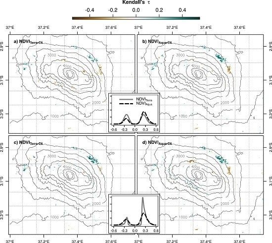
3.2.1. “Significant” Trends

Depicted in Figure 2 are the product-specific long-term trends that become evident in the study area when applying a significance level of p < 0.05 . As regards NDVI3g (Figure 2b), trend pixels largely occur spatially isolated. Greening is observable in the western and south-eastern lowlands and along the western mountainside, whereas browning is limited to a sole patch in the north and the summit area. The remaining MODIS products (Figure 2c–f), on the other hand, reveal almost uniform spatial trend patterns. Larger patches indicating greening occur distinctly outlined in the northern, north-eastern and western foothills (~2000 m). Browning, by contrast, is limited to a larger patch in the eastern foothills and to smaller areas in the northern and north-eastern upper-mountain regions (~3500 m). As opposed to NDVI3g, strong trends in positive or negative direction are hardly observable in the savanna plains.
From a more quantitative perspective, Table 2 indicates that a considerably larger amount of “significant” trends becomes apparent from the respective Collection 6 products. NDVIAqua-C6 shows an increase of 948 (or +24.8%) trend pixels as compared to NDVIAqua-C5. For NDVITerra-C6, it is still a plus of 507 (or +12.3%). However, while the number of recognizable trends increases uniformly towards Collection 6, the greening-to-browning ratio non-uniformly shifts towards more positive and negative trends for Terra-MODIS (+38.2%) and Aqua-MODIS (–3.9%), respectively. Furthermore, it becomes evident that NDVITerra-C5 as the only product under investigation yields a higher portion of browning ( 56.5 % ), whereas all remaining products are dominated by greening. This becomes particularly evident from the southern mountainside (2000 to 3500 m), where NDVITerra-C5 as the only exception documents weak, yet widespread negative trends (Figure 2c).
In addition, NDVITerra-C5 also indicates less intense greening when compared with the remaining MODIS representatives, which is particularly evident in the north-eastern foothills (Figure 2c). Indeed, we find that MDτ as a measure for the strength of simultaneously occurring trends tends to be more negative for NDVITerra-C5 (Figure 3). In a more practical sense, this means that whenever NDVITerra-C5 and another MODIS product indicate “significant” greening for one and the same pixel, the trend derived from NDVITerra-C5 tends to be less strong (up to MD τ = - 0.025 when combined with NDVITerra-C6). If both products indicate a negative trend, on the other hand, the observed browning tends to be stronger in the case of NDVITerra-C5. By contrast, MDτ effectively approaches zero when NDVITerra-C5 is not involved, thus indicating that simultaneously occurring trends are almost equal among the remaining MODIS products.

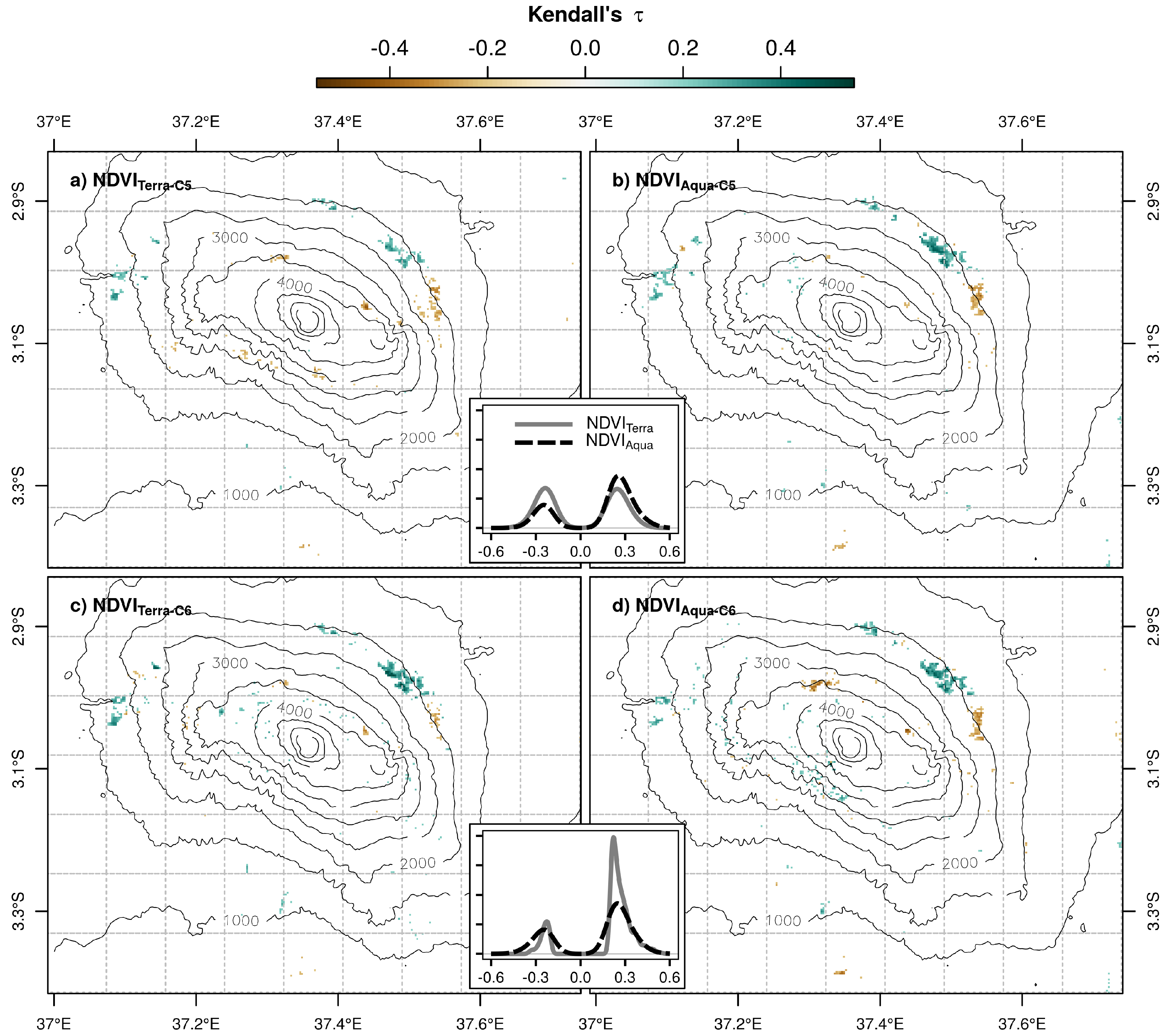
3.2.2. “Conclusive” Trends

When applying a significance level of p < 0.001 , none of the previously identified NDVI3g long-term trends remain. The 250-m MODIS products (Figure 4), on the other hand, reveal almost similar spatial patterns of “conclusive” trends when compared with Figure 2c–f except this time, the majority of less intense trends located apart from the distinct hotspot areas is masked out.
In accordance with previous findings, the number of “conclusive” trends increases towards Collection 6 (Table 3). However, while the associated growth rate remains virtually constant in the case of NDVIAqua-C6 (+25.3%), it almost doubles for NDVITerra-C6 (+21.3%). The non-uniform shift towards more positive (negative) trends in NDVITerra-C6 (NDVIAqua-C6) persists, but slightly weakens in the case of Terra-MODIS (+32.2%). In general, “conclusive” trends tend to be greener than their “significant” counterparts (Table 2), which is particularly applicable to NDVIAqua-C6 (+7.8%), NDVITerra-C5 (+7.6%) and NDVIAqua-C5 (+7.5%), whereas NDVITerra-C6 indicates only moderately increasing greenness (+1.6%).
The related values of pairwise MDτ (Figure 5) once again confirm that trends obtained from NDVITerra-C5 are distinctly biased towards smaller values of τ. However, in contrast to the results obtained from “significant” trends (Figure 3), “conclusive” trends derived from NDVITerra-C5 tend to be shifted even farther into the negative fraction. When compared with NDVITerra-C6, for instance, the trend values documented by NDVITerra-C5 are smaller by - 0.047 on average, which almost doubles the previously identified deviation between the two datasets. Slightly increasing differences also become apparent between NDVITerra-C6 and NDVIAqua-C6, which now total 0.013 in favor of the former (as compared to 0.009 in Figure 3).

3.2.3. Implications of the Significance Level on FDR

The heatmaps depicted in Figure 6 illustrate the resulting range of FDR for varying values of the power of the applied test (from 0.5 to 1.0 ) and the actual prevalence of monotonic long-term trends (from 0.0 to 0.3 ) split by “significant” (Figure 6a) and “conclusive” trends (Figure 6b). For the chosen range of values, the FDR range associated with “significant” trends is disproportionately higher ( 0.107 to 0.952 ) than the one associated with “conclusive” trends ( 0.002 to 0.283 ). Or, to say it more practically, the amount of falsely rejected null hypotheses, or false positives, or type-I errors, present in the determined “significant” trends (Table 2) outweighs the amount of false positives associated with “conclusive” trends (Table 3) by far. If we estimate, for instance, that the power of the Mann–Kendall test equals 0.8 and real trends make up 5 % of the study area, the FDR associated with “significant” trends equals 52.6 % . By contrast, a much smaller amount of type-I errors occurs when considering “conclusive” trends only ( 2.2 % ).

4. Discussion

4.1. Seasonality

The pairwise IOAs (Table 1) testifies that seasonal variations agree reasonably well across all MODIS products. Peak values are reached when combining different collections of one and the same sensor, indicating that the seasonal component remained largely untouched by the recent version update to Collection 6. In our opinion, the slightly larger deviations between Terra-MODIS and Aqua-MODIS originate from the different times of satellite overpass associated with markedly different atmospheric conditions. Duane et al. [50], for instance, emphasize that cloud formation in the area is subject to pronounced diurnal forcing, with cloud dissipation during the morning (Terra overpass; i.e., higher chance of a cloud-free view) and reformation in the afternoon (Aqua overpass).
The considerable decline in IOAs when in conjunction with NDVI3g can best be explained on the basis of Figure 1b,c. The depicted 8-km datasets agree reasonably well across the savanna plains in north-eastern and south-western direction but reveal increasing dissimilarities when approaching the mountain. While the latter phenomenon seems to be of particular severity along the southern and western mountainside, the underlying reasons for the identified spatial gradient are possibly twofold.
Firstly, the degree of association per grid cell depends on an unambiguous seasonal signal. The savanna plains reveal such a clear phenological cycle since they are strongly linked with the bimodal annual rainfall distribution [51]. For the entire north-eastern quarter of the study area, for instance, Detsch et al. [11] reported long-term seasonal amplitudes in the range of 0.2 between the long rains and the pronounced dry season. Our interpretation is thereby well in line with Fensholt and Proud [6] who, in a global context, confirmed a good agreement between Terra-MODIS and GIMMS NDVI in areas with a distinct phenological cycle. The montane forest belt, by contrast, shows a constantly high intra-annual NDVI with small-scale variations being attributable to signal noise rather than natural fluctuations [52], and thus has a dampening effect on the level of association.
Secondly, we argue that the IOAs is associated with the degree of sub-pixel heterogeneities. In the north-eastern and south-western savanna plains, narrow quantile bands indicate a mostly homogeneous pixel composition. The NDVI signal of both datasets is thus fed by one dominant land cover type which results in the highest IOAs observable in the study area. In the north-western lowlands and when approaching the mountain, however, the landscape becomes more heterogeneous as a consequence of intense land management in the foothills of Mt. Kilimanjaro encompassing e.g., widespread coffee plantations [53], intensely managed Chagga homegardens in the South [18] and broad agroforestry systems in the West [11]. When moving further uphill along the climatic gradient [14], the mountain’s geometry leads to an under-representation of the upper, spatially less extended regions in the coarse 8-km grid. Considering such small-scale transitions between predominant land covers, which particularly applies to the fragmented foothill areas, spatial resampling of the 1.1-km LAC input data to the regular 8-km GIMMS grid leads to a dilution of the unique, yet small-scale NDVI signals and the seasonality associated therewith. The same applies for spatially resampled NDVIAqua-C5 CMG data which, possibly due to the differing input data and aggregation method, considerably deviates from NDVI3g in the more heterogeneous areas. The 250-m MODIS products, on the other hand, preserve such small-scale signals and hence range on a considerably higher level of association.

4.2. Long-Term Monotonic Trends

The largest differences between “significant” and “conclusive” trends become evident from NDVI3g. When p < 0.05 applies, trends largely occur rather isolated in the outer rim of the study area, where none of the other products indicates relevant results. Moreover, the sharply outlined patches in the north-eastern and western foothills (Figure 2c–f) are not reflected by NDVI3g at all. Considering our tentative example calculation of the FDR depicted above (Section 3.2.3), we argue that more than half of all “significant” trends derived from NDVI3g can be expected to represent false alarms. Our interpretation is supported by the non-existing “conclusive” NDVI3g trends where, according to our calculations, the presence of false positives should be significantly reduced. Therefore, we conclude that (a) “significant” NDVI3g trends in the study area primarily originate from random chance; and (b) small-scale trends as documented by MODIS cannot be adequately captured by NDVI3g. Evidence for the latter finding comes e.g., from Yin et al. [54] who attributed differences between GIMMS and Satellite Pour l’Observation de la Terre (SPOT) Vegetation long-term trends to the GIMMS-specific resampling procedure from 1.1-km LAC input data to a regular 8-km grid [55]. Indeed, it seems reasonable to assume that the rather small sample size of n = 63 NDVI3g pixels covering the study area cannot adequately capture long-term vegetation dynamics in such a highly heterogeneous landscape [14]. Nonetheless, it has to be emphasized that such regional-scale findings do not necessarily apply to larger and more homogeneous areas with a smaller amount of sub-pixel heterogeneities associated with NDVI3g.
The most evident finding from the remaining MODIS products is the enhanced proportion of browning observable from NDVITerra-C5. This is not only testified by the depicted relative trend amounts (Table 2 and Table 3), but also by the calculated MDτ that indicates a negative shift of all trends identified from NDVITerra-C5, particularly when p < 0.001 applies (Figure 5). As mentioned at the beginning, this finding can be attributed to sensor degradation heavily impacting the red and near infra-red Terra-MODIS bands. Analyzing annual NDVI trends over North America, Wang et al. [8] demonstrated a very similar predominance of browning derived from NDVITerra-C5 when compared with NDVIAqua-C5. The same phenomenon has only recently been evidenced for the global scale and with particular severity identified over humid and dry-subhumid zones [56].
Our interpretation is further supported by the markedly smaller portion of browning trends in NDVITerra-C6 that possibly results from the adjusted band ageing calibration approach taken by the new Collection 6 product algorithm [9]. It remains beyond the scope of this study, however, whether the massive greening peaks found for NDVITerra-C6 (as seen from the density distributions in Figure 2 and Figure 4) indicate a possible overcompensation of Terra-MODIS sensor degradation in Collection 6. The finding that comparably large deviations do not become evident from the two Aqua-MODIS products might reinforce such an “overcompensation theory” impacting—and markedly raising—the number of Terra-based greening trends.
Apart from such tentative considerations and while the determined greening-to-browning ratios remain constant across the applied significance levels, the absolute amounts of MODIS-based trends sharply decline from the “significant” to the “conclusive” domain. Considering the above FDR estimates of 52.6 % and 2.2 % associated therewith, we argue that “significant” trends cannot be unambiguously divided into real discoveries (i.e., true positives) or random chance (i.e., false positives). Such a differentiation is far more reliable when dealing with “conclusive” trends of which an estimated proportion of 97.8 % can be assumed to reflect real conditions. Therefore, we recommend future studies to employ a significance level of p < 0.001 in order to deduce reliable long-term trends from spatially discrete time series based upon the Mann–Kendall test or, to stick with Colquhoun [44] (p. 12),
“If you want to avoid making a fool of yourself very often, do not regard anything greater than p < 0.001 as a demonstration that you have discovered something. Or, slightly less stringently, use a three-sigma rule.”
As an alternative, a sufficiently reliable distinction between real and randomly introduced trends can also be achieved by involving contextual information from neighboring locations, which is particularly valid for shorter time scales and noise-prone data. Neeti and Eastman [36], who developed a so-called “Contextual Mann–Kendall test”, pointed out that for a given trend location, a higher degree of confidence could be achieved when similar trends occurred in adjacent locations—or, to put it the other way round, a spatially isolated trend is more likely to originate from either random chance or the effects of insufficiently masked cloud remnants when no neighboring trends are observable. Since such contaminants have been sufficiently accounted for (Section 2.2.1) and, more importantly, the applied Whittaker smoother [26] largely eliminates the effects of non-captured clouds by downweighting explicitly small values, we argue that the chosen Mann–Kendall approach, which takes into account one-dimensional pixel time series only, proves sufficient for the purposes of this study.

5. Conclusions

The aim of this study was to deduce and compare seasonal and long-term NDVI dynamics over the Kilimanjaro region, Tanzania, derived from Terra-MODIS and Aqua-MODIS, Collections 5 and 6, and the 3rd Generation AVHRR GIMMS product. In this prospect, particular attention was devoted to the impacts of the chosen significance level on the estimated amounts of misclassified trends. The obtained results can be summarized as follows:
  • In terms of seasonality, the respective MODIS sensors agreed best across collections indicating that the seasonal signal largely remained unaffected by the recent product update. Across sensors, the IOAs slightly decreased which was attributed to the different timing of Terra and Aqua overpasses.
  • When MODIS was combined with GIMMS, a spatial gradient became apparent ranging from high IOAs in savanna to low IOAs when approaching the mountain. This was possibly owing to (a) the loss of a clear phenological cycle when moving towards the mountain; and (b) an increasing level of sub-pixel heterogeneities that could not be adequately captured by the 8-km GIMMS grid.
  • As concerns long-term monotonic trends, we found that the coarse resolution of GIMMS tended to dilute small-scale signals that were adequately captured by MODIS. Moreover, no GIMMS trends remained when considering “conclusive” trends ( p < 0.001 ), suggesting that the bulk of identified “significant” trends ( p < 0.05 ) was introduced by random chance rather than reflecting real trends.
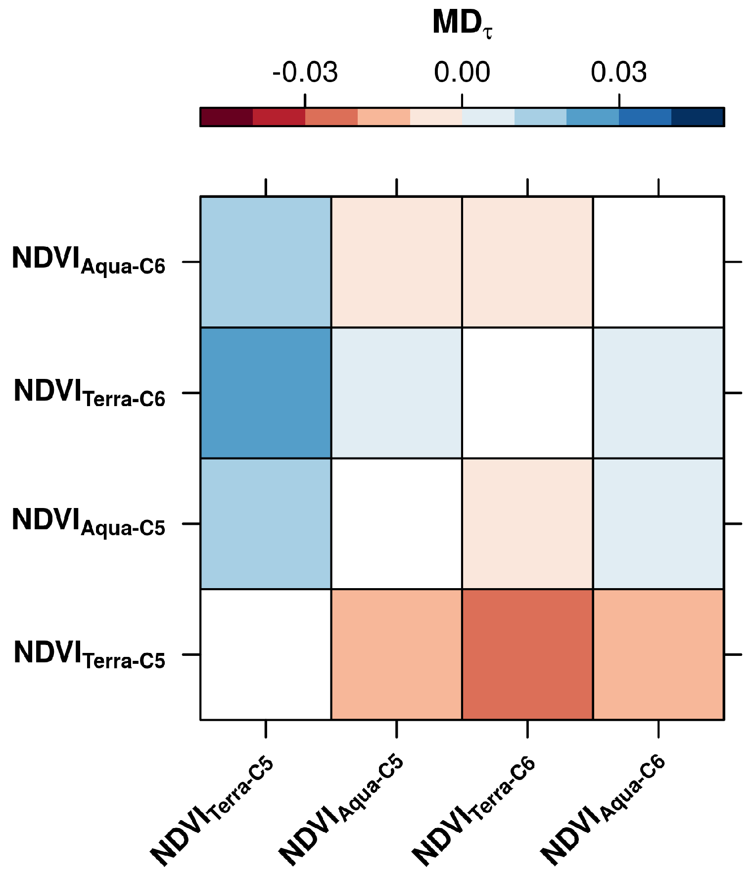
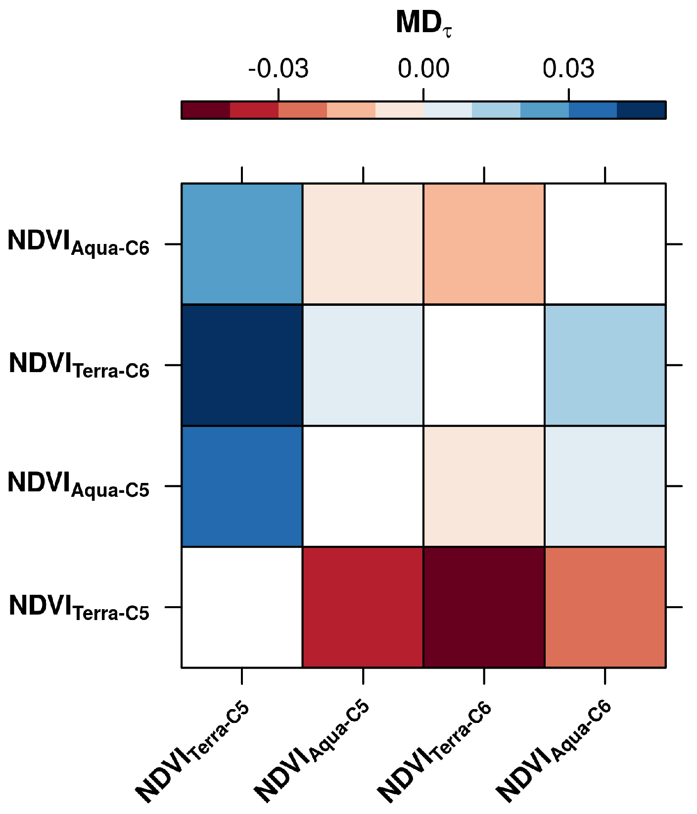
  • NDVITerra-C5 revealed distinctly more browning (and also less intense greening) than the other MODIS products as a consequence of sensor degradation. Such effects were found to vanish for NDVITerra-C6 suggesting that the new calibration approach accounts for band ageing. However, the finding that a distinctly higher portion of greening becomes apparent from NDVITerra-C6 when directly compared with NDVIAqua-C6 requires further investigation of a possible overcompensation of Terra-MODIS band ageing in Collection 6.
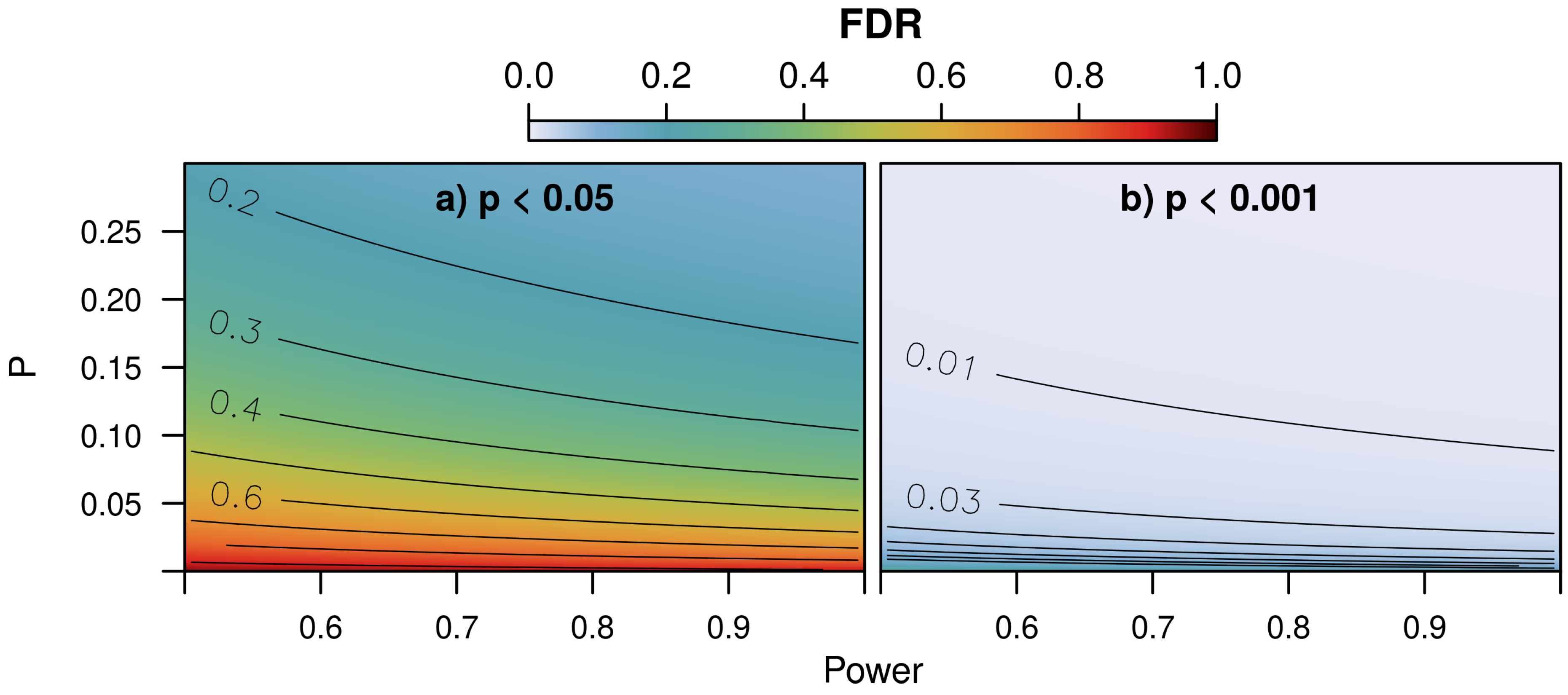
  • As seen from the FDR, the relative amount of false alarms in the trend fraction heavily depended upon the applied p-value. For instance, if we estimated the power of the Mann–Kendall test to be 0.8 and real trends to make up 5 % of the study area, then 52.6 % of all “significant” trends and only 2.2 % of all “conclusive” trends were assumed to originate from random chance.
We therefore recommend future studies targeting at the deduction of reliable long-term trends to restrict themselves to the use of p < 0.001 and/or additionally employ contextual geographical information [36] in order to minimize the occurrence of false positives. In this context, the combination of NDVITerra-C6 and NDVIAqua-C6 to derive long-term and seasonal dynamics from a doubled temporal coverage seems reasonable. However, we strongly advise to exclusively rely on NDVIAqua-C5 if, for any reason, it is required to perform analyses upon MODIS Collection 5 data.
Due to the partly massive differences that occur when comparing MODIS with GIMMS, we conclude that the coarse spatial resolution of the latter hampers a reliable deduction of seasonal and long-term dynamics in areas with a highly dynamic relief. In order to overcome these limitations and make use of such an invaluable archive of long-term vegetation dynamics, we encourage future research to combine GIMMS with the high-quality MODIS Collection 6 products to create datasets with a long-term temporal and considerably high spatial coverage. A handful of potential solutions are already available and include, amongst others, the Vegetation Index and Phenology dataset proposed by Barreto-Munoz [57] (e.g., comprehensively validated on a global scale in Tian et al. [56]) or the empirical orthogonal teleconnections-based approach recently presented by Detsch et al. [11].

Acknowledgments

This study was carried out in the framework of the research unit “Kilimanjaro ecosystems under global change: Linking biodiversity, biotic interactions and biogeochemical ecosystem processes” (KiLi; https://www.kilimanjaro.biozentrum.uni-wuerzburg.de/, accessed on 14 January 2016), and we would like to express our sincere thanks to the German Research Foundation (DFG) for the provision of funding (funding id Ap 243/1-2, Na 783/5-1, Na 783/5-2).

Author Contributions

F.D. performed data pre-processing and analyses, wrote the first draft of the manuscript and implemented most of the changes that emerged from the peer-review stage; I.O., T.A. and T.N. significantly contributed to the finally submitted and revised versions of the manuscript.

Conflicts of Interest

The authors declare no conflict of interest.

References

  1. Tucker, C.J. Red and photographic infrared linear combinations for monitoring vegetation. Remote Sens. Environ. 1979, 8, 127–150. [Google Scholar] [CrossRef]
  2. Alcaraz-Segura, D.; Chuvieco, E.; Epstein, H.E.; Kasischke, E.S.; Trishchenko, A. Debating the greening vs. browning of the North American boreal forest: Differences between satellite datasets. Glob. Chang. Biol. 2010, 16, 760–770. [Google Scholar] [CrossRef]
  3. Tucker, C.; Pinzon, J.; Brown, M.; Slayback, D.; Pak, E.; Mahoney, R.; Vermote, E.; El Saleous, N. An extended AVHRR 8-km NDVI dataset compatible with MODIS and SPOT vegetation NDVI data. Int. J. Remote Sens. 2005, 26, 4485–4498. [Google Scholar] [CrossRef]
  4. Latifovic, R.; Trishchenko, A.; Chen, J.; Park, W.B.; Khlopenkov, K.V.; Fernandes, R.; Pouliot, D.; Ungureanu, C.; Luo, Y.; Wang, S.; et al. Generating historical AVHRR 1 km baseline satellite data records over Canada suitable for climate change studies. Can. J. Remote Sens. 2005, 31, 324–346. [Google Scholar] [CrossRef]
  5. Helsel, D.R.; Hirsch, R.M. Statistical Methods in Water Resources (Techniques of Water-Resources Investigation, Book 4, Chapter A3); Elsevier: Amsterdam, The Netherlands, 2002; pp. 338–340. [Google Scholar]
  6. Fensholt, R.; Proud, S.R. Evaluation of Earth Observation based global long term vegetation trends—Comparing GIMMS and MODIS global NDVI time series. Remote Sens. Environ. 2012, 119, 131–147. [Google Scholar] [CrossRef]
  7. Guay, K.C.; Beck, P.S.; Berner, L.T.; Goetz, S.J.; Baccini, A.; Buermann, W. Vegetation productivity patterns at high northern latitudes: A multi-sensor satellite data assessment. Glob. Chang. Biol. 2014, 20, 3147–3158. [Google Scholar] [CrossRef] [PubMed]
  8. Wang, D.; Morton, D.; Masek, J.; Wu, A.; Nagol, J.; Xiong, X.; Levy, R.; Vermote, E.; Wolfe, R. Impact of sensor degradation on the MODIS NDVI time series. Remote Sens. Environ. 2012, 119, 55–61. [Google Scholar] [CrossRef]
  9. Lyapustin, A.; Wang, Y.; Xiong, X.; Meister, G.; Platnick, S.; Levy, R.; Franz, B.; Korkin, S.; Hilker, T.; Tucker, J.; et al. Scientific impact of MODIS C5 calibration degradation and C6+ improvements. Atmos. Meas. Tech. 2014, 7, 4353–4365. [Google Scholar] [CrossRef]
  10. Didan, K.; Munoz, A.B.; Solano, R.; Huete, A. MODIS Vegetation Index User’s Guide (MOD13 Series); Version 3.0.0 (Collection 6); Vegetation Index and Phenology Lab, The University of Arizona: Tucson, AZ, USA, 2015. [Google Scholar]
  11. Detsch, F.; Otte, I.; Appelhans, T.; Nauss, T. Seasonal and long-term vegetation dynamics from NDVI time series at Mt. Kilimanjaro, Tanzania. Remote Sens. Environ. 2016. under review. [Google Scholar]
  12. Pinzon, J.E.; Tucker, C.J. A non-stationary 1981-2012 AVHRR NDVI3g time series. Remote Sens. 2014, 6, 6929–6960. [Google Scholar] [CrossRef]
  13. Appelhans, T.; Mwangomo, E.; Otte, I.; Detsch, F.; Nauss, T.; Hemp, A. Eco-Meteorological Characteristics of the Southern Slopes of Mt. Kilimanjaro, Tanzania. Int. J. Climatol. 2015. in Press. Available online: http://0-onlinelibrary-wiley-com.brum.beds.ac.uk/doi/10.1002/joc.4552/full (accessed on 20 January 2016). [Google Scholar]
  14. Buytaert, W.; Cuesta-Camacho, F.; Tobón, C. Potential impacts of climate change on the environmental services of humid tropical alpine regions. Glob. Ecol. Biogeogr. 2011, 20, 19–33. [Google Scholar] [CrossRef]
  15. Hemp, A. Climate change-driven forest fires marginalize the impact of ice cap wasting on Kilimanjaro. Glob. Chang. Biol. 2005, 11, 1013–1023. [Google Scholar] [CrossRef]
  16. Otte, I.; Detsch, F.; Mwangomo, E.; Nauss, T.; Appelhans, T. Decadal trends and interannual variability of atmospheric parameters as observed from local and remote sensing time series at Mt. Kilimanjaro, Tanzania. Clim. Dyn. 2016. under review. [Google Scholar]
  17. Oettli, P.; Camberlin, P. Influence of topography on monthly rainfall distribution over East Africa. Clim. Res. 2005, 28, 199–212. [Google Scholar] [CrossRef]
  18. Hemp, A. Vegetation of Kilimanjaro: Hidden endemics and missing bamboo. Afr. J. Ecol. 2006, 44, 305–328. [Google Scholar] [CrossRef]
  19. Maeda, E.E.; Hurskainen, P. Spatiotemporal characterization of land surface temperature in Mount Kilimanjaro using satellite data. Theor. Appl. Climatol. 2014, 118, 497–509. [Google Scholar] [CrossRef]
  20. Huete, A.; Didan, K.; Miura, T.; Rodriguez, E.P.; Gao, X.; Ferreira, L.G. Overview of the radiometric and biophysical performance of the MODIS vegetation indices. Remote Sens. Environ. 2002, 83, 195–213. [Google Scholar] [CrossRef]
  21. Solano, R.; Didan, K.; Jacobson, A.; Huete, A. MODIS Vegetation Index User’s Guide (MOD13 Series); Version 2.00, May 2010 (Collection 5); Vegetation Index and Phenology Lab, The University of Arizona: Tucson, AZ, USA, 2010. [Google Scholar]
  22. LPDAAC. NASA Land Data Products and Services. Available online: https://lpdaac.usgs.gov/ (accessed on 20 January 2016).
  23. MODIS Land Team: MODIS Grids. Available online: http://modis-land.gsfc.nasa.gov/MODLAND_grid.html (accessed on 20 January 2016).
  24. MODIS Land Team: MODIS News. Available online: http://modis-land.gsfc.nasa.gov/news.html (accessed on 20 January 2016).
  25. Hyndman, R.J. Forecast: Forecasting Functions for Time Series and Linear Models. Available online: http://rpackages.ianhowson.com/cran/forecast/ (accessed on 7 December 2015).
  26. Atzberger, C.; Eilers, P.H. A time series for monitoring vegetation activity and phenology at 10-daily time steps covering large parts of South America. Int. J. Digit. Earth 2011, 4, 365–386. [Google Scholar] [CrossRef]
  27. Wittich, K.P.; Hansing, O. Area-averaged vegetative cover fraction estimated from satellite data. Int. J. Biometeorol. 1995, 38, 209–215. [Google Scholar] [CrossRef]
  28. Brown, M.E.; Pinzon, J.E.; Didan, K.; Morisette, J.T.; Tucker, C.J. Evaluation of the Consistency of Long-Term NDVI Time Series Derived From AVHRR, SPOT-Vegetation, SeaWIFS, MODIS, and Landsat ETM+ Sensors. IEEE Trans. Geosci. Remote Sens. 2006, 44, 1787–1793. [Google Scholar] [CrossRef]
  29. ECOCAST. Data Directory. Available online: http://ecocast.arc.nasa.gov/data/pub/gimms/3g.v0/ (accessed on 20 January 2016).
  30. Zhu, L.; Meng, J. Determining the relative importance of climatic drivers on spring phenology in grassland ecosystems of semi-arid areas. Int. J. Biometeorol. 2015, 59, 237–248. [Google Scholar] [CrossRef] [PubMed]
  31. Detsch, F. Gimms: Download and Process GIMMS NDVI3g Data. Available online: http://CRAN.R-project.org/package=gimms (accessed on 20 January 2016).
  32. Matloff, N. The Art of R Programming; No Starch Press: San Francisco, CA, USA, 2011; pp. 49–51. [Google Scholar]
  33. Appelhans, T.; Detsch, F.; Nauss, T. remote: Empirical Orthogonal Teleconnections in R. J. Stat. Softw. 2015, 65, 1–19. [Google Scholar] [CrossRef]
  34. de Jong, R.; de Bruin, S.; de Wit, A.; Schaepman, M.E.; Dent, D.L. Analysis of monotonic greening and browning trends from global NDVI time-series. Remote Sens. Environ. 2011, 115, 692–702. [Google Scholar] [CrossRef] [Green Version]
  35. Yue, S.; Pilon, P.; Phinney, B.; Cavadias, G. The influence of autocorrelation on the ability to detect trend in hydrological series. Hydrol. Process. 2002, 16, 1807–1829. [Google Scholar] [CrossRef]
  36. Neeti, N.; Eastman, J.R. A Contextual Mann–Kendall Approach for the Assessment of Trend Significance in Image Time Series. Trans. GIS 2011, 15, 599–611. [Google Scholar] [CrossRef]
  37. Sen, P.K. Estimates of the Regression Coefficient Based on Kendall’s Tau. J. Am. Stat. Assoc. 1968, 63, 1379–1389. [Google Scholar] [CrossRef]
  38. Bronaugh, D.; Werner, A. Zyp: Zhang + Yue-Pilon Trends Package. Available online: http://CRAN.R-project.org/package=zyp (accessed on 20 January 2016).
  39. Mann, H.B. Nonparametric tests against trend. Econometrica 1945, 13, 245–259. [Google Scholar] [CrossRef]
  40. Kendall, M.G. A new measure of rank correlation. Biometrika 1938, 30, 81–93. [Google Scholar] [CrossRef]
  41. Meals, D.W.; Spooner, J.; Dressing, S.A.; Harcum, J.B. Statistical Analysis for Monotonic Trends; Tech Notes 6; National Nonpoint Source Monitoring Program: Fairfax, VA, USA, 2011; pp. 1–23. [Google Scholar]
  42. McLeod, A.I. Kendall: Kendall Rank Correlation and Mann–Kendall Trend Test. Available online: http://CRAN.R-project.org/package=Kendall (accessed on 20 January 2016).
  43. Önöz, B.; Bayazit, M. The Power of Statistical Tests for Trend Detection. Turk. J. Eng. Environ. Sci. 2003, 27, 247–251. [Google Scholar]
  44. Colquhoun, D. An investigation of the false discovery rate and the misinterpretation of p-values. R. Soc. Open Sci. 2014, 1. [Google Scholar] [CrossRef] [PubMed]
  45. Benjamini, Y.; Hochberg, Y. Controlling the False Discovery Rate: A Practical and Powerful Approach to Multiple Testing. J. R. Stat. Soc. Ser. B 1995, 57, 289–300. [Google Scholar]
  46. Miller, D.A. “Significant” and “Highly Significant”. Nature 1966, 210, 1190. [Google Scholar] [CrossRef] [PubMed]
  47. Map Data: Google, TerraMetrics. Available online: http://maps.googleapis.com/maps/api/staticmap?center=-3.123553240247,37.366348380164&zoom=10&size=640x497&maptype=satellite&format=gif&sensor=false&scale=2 (accessed on 20 January 2016).
  48. Ong’injo, J.; (Deputy registrar, Kisumu); Lambrechts, C.; (United Nations Environment Programme); Hemp, A.; (Plant physiology, University of Bayreuth). Personal communication, 2015.
  49. OpenStreetMap. Copyright and License. Available online: http://www.openstreetmap.org/copyright (accessed on 20 January 2016).
  50. Duane, W.J.; Pepin, N.C.; Losleben, M.L.; Hardy, D.R. General Characteristics of Temperature and Humidity Variability on Kilimanjaro, Tanzania. Arct. Antarct. Alp. Res. 2008, 40, 323–334. [Google Scholar] [CrossRef]
  51. Ivory, S.J.; Russell, J.; Cohen, A.S. In the hot seat: Insolation, ENSO, and vegetation in the African Tropics. J. Geophys. Res. Biogeosci. 2013, 118, 1347–1358. [Google Scholar] [CrossRef]
  52. Huete, A.R.; Saleska, S.R. Remote Sensing of Tropical Forest Phenology: Issues and Controversies. Int. Arch. Photogramm. Remote Sens. Spat. Inf. Sci. 2010, 38, 539–541. [Google Scholar]
  53. Rutten, G.; Ensslin, A.; Hemp, A.; Fischer, M. Vertical and Horizontal Vegetation Structure across Natural and Modified Habitat Types at Mount Kilimanjaro. PLoS ONE 2015, 10, e0138822. [Google Scholar] [CrossRef] [PubMed]
  54. Yin, H.; Udelhoven, T.; Fensholt, R.; Pflugmacher, D.; Hostert, P. How Normalized Difference Vegetation Index (NDVI) Trends from Advance Very High Resolution Radiometer (AVHRR) and Système Probatoire d’Observation de la Terre VEGETATION (SPOT VGT) Time Series Differ in Agricultural Areas: An Inner Mongolian Case Study. Remote Sens. 2012, 4, 3364–3389. [Google Scholar] [CrossRef]
  55. Kidwell, K.B. NOAA POLAR ORBITER DATA USER’S GUIDE (TIROS-N, NOAA-6, NOAA-7, NOAA-8, NOAA-9, NOAA-10, NOAA-11, NOAA-12, NOAA-13 AND NOAA-14). Available online: https://www.ncdc.noaa.gov/oa/pod-guide/ncdc/docs/podug/index.htm (accessed on 20 January 2016).
  56. Tian, F.; Fensholt, R.; Verbesselt, J.; Grogan, K.; Horion, S.; Wang, Y. Evaluating temporal consistency of long-term global NDVI datasets for trend analysis. Remote Sens. Environ. 2015, 163, 326–340. [Google Scholar] [CrossRef]
  57. Barreto-Munoz, A. Multi-Sensor Vegetation Index and Land Surface Phenology Earth Science Data Records in Support of Global Change Studies: Data Quality Challenges and Data Explorer System. Ph.D. Thesis, Department of Agricultural and Biosystems Engineering, The University of Arizona, Tucson, AZ, USA, 2013. [Google Scholar]
Figure 1. (a) Spatial coverage of the 1/12-degree GIMMS grid (white dashed) including consecutive pixel numbering superimposed upon an aerial image of the study area (Map data: Google, TerraMetrics [47]); (b) spatial pattern of IOAs between NDVI3g and MODIS CMG-based NDVIAqua-C5 (Section 2.2.1); (c) raw time series (2003–2012) of NDVI3g (purple) and MODIS CMG-based NDVIAqua-C5 (orange) including 10%–90% quantile range calculated from all 250-m NDVIAqua-C5 pixels falling inside each 8-km GIMMS pixel (light orange). The underlying coordinate reference system (CRS) in (a) and (b) is EPSG:4326 and the digital elevation model (black solid) is based on toposheets at scale 1:50000 digitized by Ong’injo et al. [48].
Remotesensing 08 00159 g001
Figure 2. (a) Bing Maps aerial image of the study area (downloaded via OpenStreetMap [49]); spatial patterns of “significant” values of τ (2003–2012) for (b) NDVI3g; (c) NDVITerra-C5; (d) NDVIAqua-C5; (e) NDVITerra-C6; and (f) NDVIAqua-C6. Also included are the 1-d Kernel density estimates for the 250-m MODIS products originating from Collections 5 (connecting c and d) and 6 (connecting e and f). The underlying CRS and additional data are the same as in Figure 1.
Remotesensing 08 00159 g002
Figure 3. MDτ calculated from “significant” values of τ ( p < 0.05 ) for each pair of MODIS NDVI products.
Remotesensing 08 00159 g003
Figure 4. Spatial patterns of “conclusive” values of τ (2003–2012) for (a) NDVITerra-C5; (b) NDVIAqua-C5; (c) NDVITerra-C6; and (d) NDVIAqua-C6. Also included are the 1-d Kernel density estimates for the 250-m MODIS products originating from Collections 5 (connecting a and b) and 6 (connecting c and d). The underlying CRS and additional data are the same as in Figure 1.
Remotesensing 08 00159 g004
Figure 5. MDτ calculated from “conclusive” values of τ ( p < 0.001 ) for each pair of MODIS NDVI products.
Remotesensing 08 00159 g005
Figure 6. FDR depending on the Power of the applied test and the trend prevalence (P) under real conditions for (a) “significant” trends ( p < 0.05 ); and (b) “conclusive” trends ( p < 0.001 ).
Remotesensing 08 00159 g006
Table 1. Mean IOAs for all possible product combinations (see e.g., Figure 1b for pixel-wise IOAs between NDVI3g and NDVIAqua-C5 from which the mean value of 0.776 denoted herein is calculated). IOAs involving NDVI3g is calculated from the MODIS CMG products (Section 2.2.1), whereas MODIS-only IOAs is derived from the 250-m products.
NDVI3gNDVITerra-C5NDVIAqua-C5NDVITerra-C6NDVIAqua-C6
NDVI3g1
NDVITerra-C50.7501
NDVIAqua-C50.7760.8111
NDVITerra-C60.7450.8610.8071
NDVIAqua-C60.7360.8010.8530.8041
Table 2. Product-specific pixel amounts of “significant” monotonic trends ( p < 0.05 ; Figure 2).
Trend PixelsTrends (%)Greening (%)Browning (%)
NDVI3g80.1270.7500.250
NDVITerra-C541240.0440.4350.565
NDVIAqua-C538170.0400.6540.346
NDVITerra-C646310.0490.8170.183
NDVIAqua-C647650.0500.6150.385
Table 3. Product-specific pixel amounts of “conclusive” monotonic trends ( p < 0.001 ; Figure 4).
Trend PixelsTrends (%)Greening (%)Browning (%)
NDVI3g00
NDVITerra-C56070.0060.5110.489
NDVIAqua-C57120.0080.7290.271
NDVITerra-C67360.0080.8330.167
NDVIAqua-C68920.0090.6930.307

