Comparing and Combining Remotely Sensed Land Surface Temperature Products for Improved Hydrological Applications

Abstract

Land surface temperature (LST) is an important variable that provides a valuable connection between the energy and water budget and is strongly linked to land surface hydrology. Space-borne remote sensing provides a consistent means for regularly observing LST using thermal infrared (TIR) and passive microwave observations each with unique strengths and weaknesses. The spatial resolution of TIR based LST observations is around 1 km, a major advantage when compared to passive microwave observations (around 10 km). However, a major advantage of passive microwaves is their cloud penetrating capability making them all-weather sensors whereas TIR observations are routinely masked under the presence of clouds and aerosols. In this study, a relatively simple combination approach that benefits from the cloud penetrating capacity of passive microwave sensors was proposed. In the first step, TIR and passive microwave LST products were compared over Australia for both anomalies and raw timeseries. A very high agreement was shown over the vast majority of the country with R² typically ranging from 0.50 to 0.75 for the anomalies and from 0.80 to 1.00 for the raw timeseries. Then, the scalability of the passive microwave based LST product was examined and a pixel based merging approach through linear scaling was proposed. The individual and merged LST products were further compared against independent LST from the re-analysis model outputs. This comparison revealed that the TIR based LST product agrees best with the re-analysis data (R² 0.26 for anomalies and R² 0.76 for raw data), followed by the passive microwave LST product (R² 0.16 for anomalies and R² 0.66 for raw data) and the combined LST product (R² 0.18 for anomalies and R² 0.62 for raw data). It should be noted that the drop in performance comes with an increased revisit frequency of approximately 20% compared to the revised frequency of the TIR alone. Additionally, this comparison against re-analysis data was subdivided over Australia’s major climate zones and revealed that the relative agreement between the individual and combined LST products against the re-analysis data is consistent over these climate zones. These results are also consistent for both the anomalies and the raw time series. Finally, two examples were provided that demonstrate the proposed merging approach including an example for the Hunter Valley floods along Australia’s central coast that experienced significant flooding in April 2015.

1. Introduction

The thermodynamic temperature of the uppermost layer of the Earth’s surface is defined as land surface temperature (LST). LST is an important variable in the processes controlling energy, water and biogeochemical fluxes at the interface between the Earth’s surface and the atmosphere. Several studies indicated the very strong link of LST to land surface hydrology (e.g., [1,2,3]) and others demonstrated the potential use of remotely sensed LST as an indicator of surface inundation state [4]. In order to further study these hydrological processes, existing LST products must be refined and widely tested to routinely measure this important variable and demonstrate its usefulness for operational purposes such as warning systems. Specifically, precipitation is generally associated with cloud cover leading to the absence of thermal infrared (TIR) observations towards the most critical time period in flood warning systems, those final days leading up to an actual inundation event. Due to their cloud penetrating capacity, passive microwave observations are generally available within this critical time period and could provide further insight during such periods in which TIR observations are absent.

LST can be obtained through various sensors from visible, infrared, TIR and passive microwave channels mounted on polar orbiting satellites, equatorial orbiting satellites or geostationary satellites. A commonly used global LST product is based on TIR observations of Moderate Resolution Imaging Spectroradiometer (MODIS; [5]). MODIS is mounted onboard two National Aeronautics Space Administration (NASA) platforms that are dedicated to monitoring the state of the Earth’s environment (Terra) and the various components of the hydrological cycle (Aqua). A major limitation of the TIR observations from the MODIS sensors is obstruction by clouds and aerosols and their accuracies around cloud and aerosols edges [5]. Observations that were severely contaminated by clouds and aerosols are routinely masked, hence treated as no data values. Figure 1 provides an example of such cloud obstruction that affects the availability of the MODIS LST product, this example presents observations taken on 3 April 2015 during the day (01:30 PM). The central part of Western Australia (WA) as well as the majority of the states of South Australia (SA), New South Wales (NSW) and the Australian Capital Territory (ACT) experienced cloud cover leading to a significant number of no data values. On the other hand, a major advantage of this MODIS LST product is its high spatial resolution (around 1 km). Passive microwave observations have the capacity to penetrate clouds and are all-weather sensors. The complementary characteristics of these two remotely sensed observations allow for combining their strengths in a merged product—the high spatial resolution of the TIR and the all-weather capability of microwave observations.

As an example, operational flood warning systems are driven by precipitation as the main predictor and the initial (wetness) conditions of the land surface needs to be determined through various sources of remote sensing information [4]. Specifically for a warning system, cloud obstruction is a major limitation of TIR observations due to the strong link between clouds and precipitation generally leading to the absence of thermal infrared (TIR) observations in those final days leading up to an actual inundation event. In order to overcome this limitation within a critical time period, we aim to develop a relatively simple merging scheme that can benefit from the advantages of both TIR and passive microwave observations.

2. Land Surface Temperature Data

Several LST products were used in this study including two products obtained by space-borne remote sensing and an output of a re-analysis model to particularly increase our understanding over the various climate zones that Australia contains. The primary LST source comes from the MODIS sensor (Section 2.1) onboard the NASA Aqua satellite. The second LST data product comes from the multi frequency passive microwave sensor onboard the Japanese Aerospace eXploration Agency (JAXA) Global Chance Observation Mission-Water (GCOM-W) satellite (Section 2.2) and the re-analysis LST data product from Modern Era Retrospective-analysis for Research and Applications (MERRA; Section 2.3) which was primarily used for independent comparison purposes in this study and serves as a consistent reference to better understand spatial patterns over the entire country, particularly over the climate zones.

2.1. MODIS

Both NASA’s Terra and Aqua satellites carry MODIS sensors and were launched in 1999 and 2002, respectively. In this study, we use the LST product obtained from the MODIS sensor onboard the Aqua satellite as its local equatorial overpass time coincides with that of the GCOM-W satellite. Both (Aqua and GCOM-W) have their day time equatorial overpass around 1.30 PM (ascending) and their night time overpass around 1.30 AM (descending). The MODIS LST is at a high spatial resolution (around 1 km) compared to passive microwaves (around 10 km), however, in this study we used the MYD11C1 (MODIS Aqua) product of which the standard product is aggregated into 0.05° grid boxes. This product was further aggregated into 0.10° grid boxes to spatially match the microwave observations.

The MODIS LST product is retrieved through the split window method [5] that uses TIR channels 31 and 32. This MODIS LST product has been extensively validated against ground based observations (e.g., [6,7,8]) and radiance based validation studies. Relevant for the current study is that [7] showed the high consistency between TIR- and microwave- based LST products against ground observations over a number of sites located in the Murrumbidge catchment located in Southeast Australia, hence demonstrating the high potential for combining those remotely sensed products. In this study, the MYD11C1 LST product was further aggregated into 0.10° grid boxes to get a spatial match with the LST product derived from the Advanced Microwave Scanning Radiometer 2 (AMSR2) sensor on GCOM-W. For consistency reasons in the analyses, we only included aggregated MODIS LST data product in absence of any cloud and aerosol contamination. Furthermore, unless mentioned otherwise, a 3-year period was analyzed starting on 24 July 2012, coinciding with the start of the operational status of AMSR2, to the same calendar day in 2015. The MODIS MYD11C1 LST data was provided by the United States Geological Survey [5].

2.2. AMSR2

The AMSR2 is a multi-frequency passive microwave sensor onboard JAXA’s GCOM-W satellite. This satellite was launched on 17 May 2012 and is the first in a series that is expected to contribute to observing various aspects of the carbon and hydrological cycle including precipitation, water vapor, soil moisture, snow depths, carbon, radiation and sea water temperature. Passive microwave observations are sensitive to the land surface and water and, therefore, play an important role in observing the varying phases and quantities of water in both time and space. AMSR2 is the successor of the successful Advanced Microwave Scanning Radiometer for Earth Observing Systems (AMSR-E) that provided Earth scientists an almost decadal, consistent and continuous global passive microwave database. AMSR2 and AMSR-E have an almost identical sensor setup that covers a range of microwave frequencies, although AMSR2 was further improved based on the extensive experience with its predecessor. The spatial resolution, spectral resolution and sensor accuracies of AMSR2 were all improved and an additional C-band channel (7.3 GHz) was successfully added to mitigate artificial radio frequency interference [9].

Several approaches that link passive microwave observations to LST were developed over the recent years. Holmes et al. 2009 [10] presents a simple, general approach and compared its performance at the global scale by extensive validation against flux tower data and also provided a global comparison against modelled data. They presented an approach that related the vertically polarized Ka-band frequency channel (T_{b, 37V}) to LST through a single linear regression model with global applicability. Based on comparison against in situ observations, Holmes et al. 2009 [10] determined a threshold of 259.8 K for its global regression model—transition point under which passive microwave emissions behaves nonlinearly. Over Australia, their error simulations suggested relatively small biases generally ranging between 1.5 and −1.5 degrees [K] with the exception of the Simpson Desert located in Central Australia. In the present study, the single regression model to derive LST globally was used as described in Section 3.1, and compared against an existing LST product. In the next scaling step, a linear regression model was adopted and applied at individual pixel level as detailed in Section 3.2.

2.3. MERRA

MERRA provides a global re-analysis data record to support earth science objectives of NASA with a special emphasis on the global hydrological cycle [11]. Several diagnostics are produced at 6-hourly intervals whereas others, including LST, are produced at hourly intervals. The MERRA data product comes in a relatively coarse spatial resolution of 1/2° latitude by 2/3° longitude. In this study, MERRA serves as a consistent reference that could provide additional quality information about the individual and merged LST products. Additionally, our main interest is over large areas so Australia was subdivided into major climate zones. MERRA was used consistently over these different zones as ground based observations in isolated monitoring networks lack spatial consistency over large spatial domains [12]. This particular purpose justifies a nearest neighbor re-sampling of this coarse product to a finer grid that matches the AMSR2 observations as well as the aggregated MODIS observations. MERRA data is publically available through the Goddard Earth Sciences Data and Information Services Centre; for more information on the MERRA data, readers are directed to [11].

3. Methodology and Results

In the first step, the existing remotely sensed LST products are compared over Australia to gain a better understanding of their differences and similarities. Our analysis is focused on the temporal agreement as systematic differences may exist due to the different vertical depths that are observed; [7] hence, coefficient of determination (R²) and standard error (SE) are the metrics of interest. This SE was determined through Equation (1) in which ${\mathsf{\sigma }}_x$ represents the variation in the MODIS LST. In order to better understand seasonal trends and interannual variability, this part of the analysis was done on both anomalies after removing the climatology as well as raw timeseries. The decomposition into anomalies was done through a standard approach that uses a 31-day moving window centered on a particular day of the year following [4]. In the next step, the scalability of the passive microwave based product is examined and a relatively simple merging approach was proposed. Then, the various different LST products and the combined product were compared against the MERRA re-analysis LST dataset that serves as a consistent reference over the various climate zones that Australia experiences, again for anomalies and raw timeseries. Finally, the comparison against MERRA was divided over these four major climate zones to further understand their agreement.

$$SE={\sigma }_x\sqrt{1-R^2}$$

(1)

3.1. Comparing Existing Products

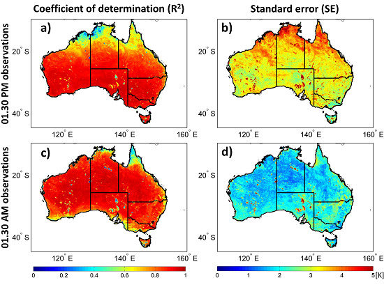
A direct comparison between the LST products from MODIS and AMSR2 was presented in order to better understand their potential differences and similarities. Figure 2 was based on the anomalies and presents both the R² (left) and the SE (right) for the observations that were taken during the day (top) and during the night (bottom). The raw time series were analyzed in an identical way and those spatial maps were presented in the supplementary material (Figure S1). Furthermore, these satellite paths were explicitly separated to understand how different physical conditions during the day and the night impact these LST products. A common assumption (e.g., [13,14]) in applications that use LST products is that the soil and canopy temperature are equal during the night due to thermal equilibrium. During the day, this assumption introduces uncertainties due to the imposed cooling effect of transpiration which generally results in soil temperatures that are higher than canopy temperatures. This phenomenon may impact the products differently as the original spatial resolution of the MODIS LST product is 1 km; hence, this product may have better ability to represent canopy and soil temperature separately than the passive microwave LST product.

For the anomalies, it was found that the mean R² values over Australia were high for both the day (R² 0.48) and night (R² 0.56) time observations. The mean R² values for the raw time series from Figure S1 were found to be even higher, for the day (R² 0.82) and night (R² 0.85) time observations. The spatial distribution of these R² values showed many similarities but also some differences for both the day and night time observations, as well as the anomalies compared to the raw time series. Generally, the products show very high agreement with R² ranging from 0.50 to 0.75 for the anomalies and from 0.8 to 1.0 for the raw time series over the central part of Australia. This agreement tends to drop in the tropical regions located in the north of Australia with relatively low agreement in the far north of WA and the Northern Territory (NT) for the day time observations and a relatively low agreement in the far north of Queensland (QLD) for the night time observations. Another feature that stands out in the R² maps is the effect that open water may have on the agreement between the products, which tends to drop significantly as shown for Lake Eyre, Lake Torrens, Lake Gairdner in SA, and Lake Mackay and Lake Argyle that border WA and the NT. Inversely, this drop in R² results in an increase in SE over these lakes and is evident in both the anomalies and raw time series as well as the different overpasses. Another feature that stands out in the SE maps is the contrast between the day and the night time maps which are reflected in the higher mean values over Australia for the day (SE 3.18 K for the anomalies) as compared to night (SE 1.88 K for the anomalies) time observations. This contrast is in agreement with the commonly used assumption (e.g., [13,14]) that was previously mentioned.

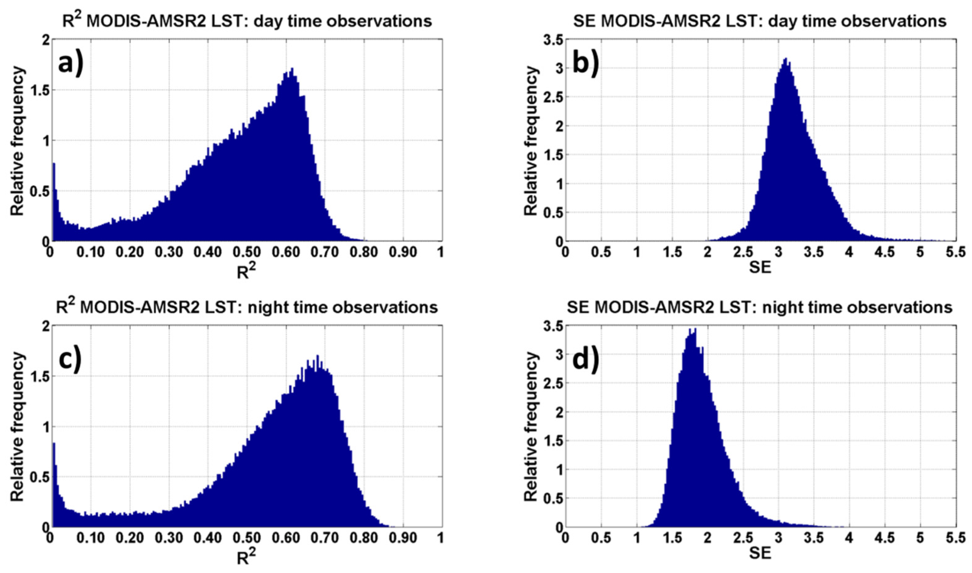
In order to further understand the comparison between both LST products, histograms that portray the relative frequency of these two metrics were also presented in a similar order as Figure 2. Figure 3 presents the distribution of R² and SE for the anomalies whereas the histograms of the raw time series were presented in in the supplementary material (Figure S2). These histograms confirm that the vast majority of R² over Australia is within the high range that was indicated earlier and that only a fraction of the analyzed pixels show a weak agreement. These histograms also confirm the contrasting agreement between the day and night-time observations with significantly lower SE values for the night time LST products. The relative differences in the histograms of the anomalies and the raw time series are also in line with expectations, particularly the overall drop in R² shifting the entire histogram to a lower range. Again, the day and night-time contrast is in agreement with earlier findings (e.g., [13,14]) on thermal equilibrium.

As previously mentioned (Section 2.2), the original passive microwave LST algorithm used a predetermined threshold to delineate frozen and unfrozen conditions. A simple analysis was conducted in order to determine the effect of such nonlinearities over our study area. The analysis as presented in Figure 2 was repeated without the implementation of this predetermined threshold for both the anomalies and raw time series. These results confirm the nonlinear behavior below this preset threshold as R² drops and SE increases in absence of the masking procedure which was shown to be consistent for day- and night-time observations (

Table 1. Mean R² and SE over Australia that demonstrates the impact of a routinely applied masking procedure over our study area. Note that the statistics for the anomalies were presented first and those for the raw timeseries were presented within brackets.

	Night Time Observations		Day Time Observations
	No Masking	Tb, 37V < 259.8 Masked	No Masking	Tb, 37V < 259.8 Masked
R2	0.561 (0.844)	0.563 (0.847)	0.478 (0.818)	0.480 (0.819)
SE	1.888 (2.012)	1.885 (2.000)	3.189 (3.461)	3.183 (3.451)

). However, this analysis also shows its marginal impact over our study area as R² is marginally higher and SE is marginally lower with the masking procedure applied. Finally, a note should be made that the impact of this masking procedure is expected to become rather significant in regions with more pronounced freezing seasons than that of Australia.

3.2. Linear Scaling of Microwave Observations

In this section, a relatively simple scaling approach is proposed which is very much in line with the general solution presented by [10] but with the explicit goal to scale the AMSR2 (T_{b, 37V}) observations in the MODIS LST product. The logic behind this experimental setup is that (1) Microwave based LST is considered to be an alternative to TIR based LST and (2) MODIS has the capabilities to observe at higher spatial resolution (up to 1 km). These two factors justify the choice to treat MODIS LST as the primary product as it would always be preferred in operational schemes due to its higher spatial resolution. We should again emphasize that the main predictor of flooding—that is, precipitation—is generally associated with cloud cover leading to the absence of thermal infrared (TIR) observations towards the most critical time period in a flood warning system. A pixel based linear regression was executed for MODIS LST and AMSR2 (T_{b, 37V}) observations, the day- and night-time observations were again explicitly analyzed separately. The slope and offsets were only determined for the raw timeseries as the decomposition into anomalies is applied in a follow on step. Figure 4 presents the slope values (left) of the pixel based linear regression and the corresponding offset values (middle) were also reported. Additionally, we also presented the sample sizes (right) within the three year analysis period used to determine the regression parameters. The spatial pattern of these sample sizes is a direct function of the (remotely sensed) revised times combined with the (natural) spatial variability of cloud cover and aerosols. Again, observations that were taken during the day (top) and during the night (bottom) were separated. In this pixel based regression analysis, there is dependence between slope and offset values which result in distinct spatial patterns. Many regions, such as the Tropical regions located in the north of Australia and the large lakes in WA, SA and the NT therefore show a distinct spatial pattern in both the slope and offset.

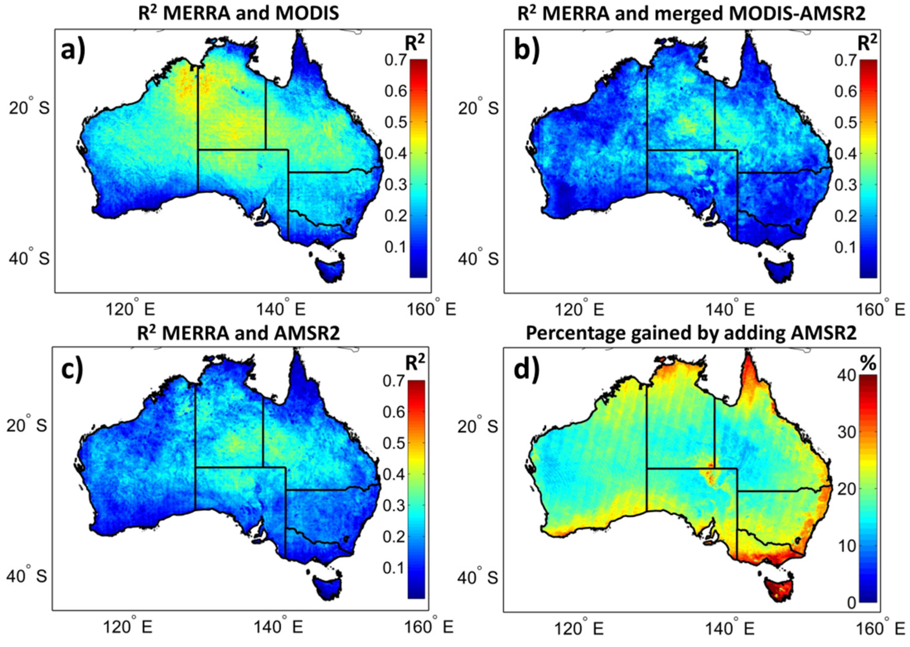
3.3. A Comparison against MERRA

The pixels based slope and offset presented in Figure 4 were now used to scale AMSR2 (T_{b, 37V}) observations into the MODIS LST product through Equation (2). Each individual pixel in time was assessed and gaps in the MODIS LST product that were caused by clouds or aerosols were, in case AMSR2 observations were available, filled through the pixels based linear regression (Equation (2)).

$$LS{T}_{Gapfilled}=slope\times T_{b,37v}+offset$$

(2)

These combined MODIS and AMSR2 time series were also deseasonalized resulting in anomalies from the combined LST product. Hence, the combined LST product benefits from the cloud penetrating capacity of the passive microwaves observations leading to an increased revisit frequency compared to the individual MODIS LST products. Here, both individual MODIS and AMSR2 products were compared against the MERRA re-analysis data as well as the combined LST products in which the scaled AMSR2 observations fill the cloud gaps in MODIS. The results from this comparison were presented in Figure 5, which shows the R² of the three different product combinations and the percentage of observations that was gained through the addition of the passive microwaves for the night-time observations alone. This comparison against MERRA was repeated for the raw time series of which the results were presented in the supplementary material (Figure S3).

The individual MODIS (Figure 5a) and the AMSR2 LST products (Figure 5c) show a very similar agreement against the independent MERRA dataset with relative high R² values over the vast majority of central Australia for both the anomalies and raw time series. When comparing results from the anomalies (Figure 5) against the raw time series (Figure S3), there is a tendency of lower R² values for the anomalies. This lower agreement is the result of removing seasonal trends hence representing the skills of the various products to represent the interannual variability. It should furthermore be noted that such a drop is in line with expectations [4] as anomalies generally demonstrate lower agreement than raw time series. The agreement between the MODIS and AMSR2 LST products and the MERRA dataset breaks in the Tropical climate zone located in the north of Australia and this is more profound for AMSR2 than it is for MODIS. In this part of Australia, it is likely difficult to observe LST through passive microwaves due to rain bearing clouds and active precipitation but land surface modelling may also suffer larger uncertainties due to convection processes [15]. Likewise, this agreement breaks for both products in Southern Victoria (VIC) and Tasmania (TAS). On the other hand, decreasing agreement between MODIS and MERRA was shown in the southern part of WA whereas AMSR2 shows moderate agreement with MERRA in these regions. Generally, the agreement between MERRA and MODIS (Figure 5a) is highest with a country average R² of 0.26 for anomalies and R² of 0.76 for raw time series followed by the AMSR2 product (R² 0.16 for anomalies and R² 0.66 for raw time series) and the combined product (R² 0.18 for anomalies and R² 0.62 for raw time series). 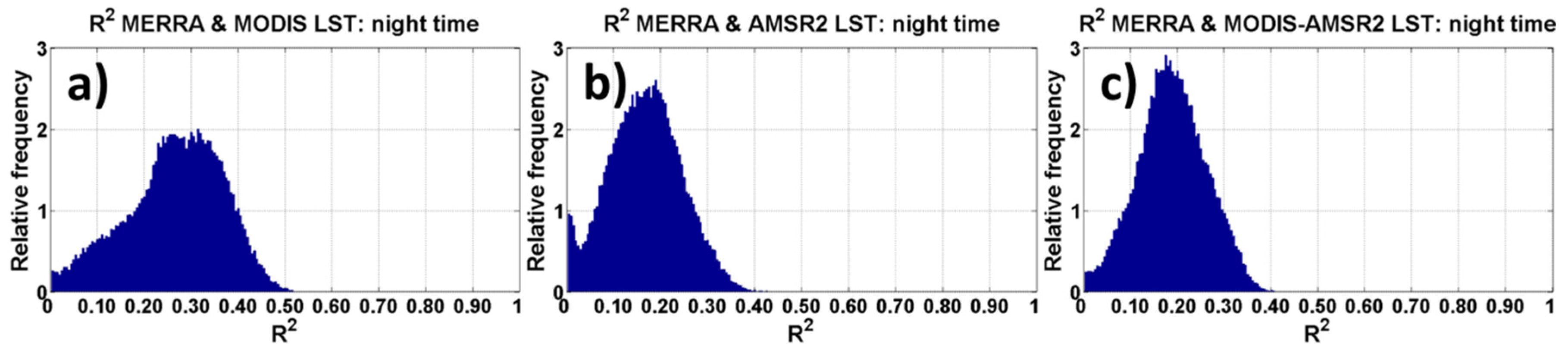Figure 6 present histograms of the results of this comparison against MERRA, again for the individual MODIS LST product (Figure 6a), the AMSR2 LST product (Figure 6b) and the combined LST product (Figure 6c). This comparison was repeated for the raw timeseries of which the results were presented in the supplementary material (Figure S4).

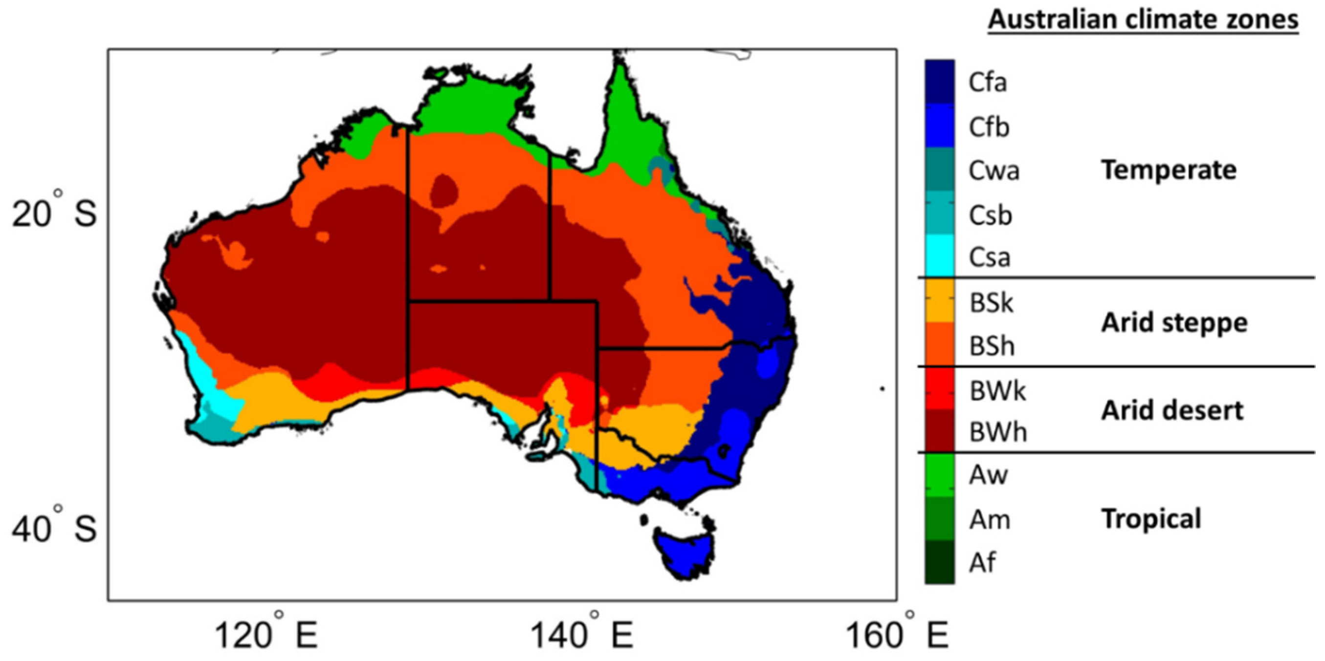
These results were furthermore divided in the different Köppen-Geiger climate zones [16] that Australia experiences, the spatial distribution of these climate zones was presented in Figure 7. These different zones are based on the original Köppen classification which was modified by [16] and consists of 29 different climate sub categories globally and 12 sub categories for Australia. These 12 Australian sub categories were divided into four major climate zones including tropical, arid desert, arid steppe and temperate. Three sub categories were merged in the tropical (A) climate zone and they include rainforest (f), monsoon (m) and Savannah (w). Furthermore, the arid desert (BW) and arid steppe (BS) were separated into a major climate zone and both consist of two different sub categories including hot (h) and cold (k). Finally, the temperate climate zone includes five different sub categories (Csa, Csb, Cwa, Cfa and Cfb) that were categorized based on drought and temperature indicators throughout the season. Figure 7 presents the spatial extent of these 12 Köppen-Geiger sub categories over Australia including the four major climate zones that were further used in this study.

Table 2. Summarized statistics for the MERRA comparison against the individual MODIS and AMSR2 LST products and the combined product in which cloud gaps in MODIS were filled with scaled AMSR2 observations. Note that the statistics for the anomalies were presented first and those for the raw timeseries were presented within brackets.

	MERRA	Climate Zone
		Tropical		Arid Desert		Arid Steppe		Temperate
		R2	SE	R2	SE	R2	SE	R2	SE
Night Time	MODIS	0.20 (0.56)	2.17 (2.52)	0.30 (0.84)	2.59 (2.74)	0.27 (0.77)	2.55 (2.78)	0.16 (0.64)	2.68 (2.85)
	AMSR2	0.12 (0.36)	3.29 (2.76)	0.19 (0.73)	3.21 (3.41)	0.16 (0.64)	3.30 (3.34)	0.11 (0.62)	3.25 (2.73)
	MODIS-AMSR2	0.11 (0.30)	2.80 (3.39)	0.22 (0.71)	3.12 (3.66)	0.19 (0.61)	3.11 (3.64)	0.13 (0.55)	2.80 (3.21)
Day Time	MODIS	0.09 (0.50)	4.02 (4.35)	0.33 (0.83)	3.63 (4.19)	0.30 (0.74)	3.95 (4.33)	0.39 (0.81)	3.52 (3.84)
	AMSR2	0.22 (0.43)	4.11 (4.58)	0.39 (0.76)	4.11 (5.29)	0.38 (0.68)	4.10 (5.13)	0.43 (0.73)	3.73 (4.73)
	MODIS-AMSR2	0.13 (0.40)	4.77 (5.58)	0.32 (0.71)	4.83 (6.03)	0.30 (0.63)	4.92 (5.93)	0.37 (0.68)	4.41 (5.58)

provides the averaged results per major climate zone and demonstrates a high degree of consistency compared to the country average results for both the anomalies and the raw time series. First, the relative agreement between MERRA and both individual and merged products is consistent with highest agreement for MODIS and the lowest agreement for the combined product, demonstrated by both R² and SE metrics. The lowest agreement for all products was generally found in the tropical climate zone followed by the temperate climate zone, arid steppe and the highest agreement was found over arid deserts. It should be emphasized that the agreement drops for the merged product comes with a significant increase (20% on average) in number of observations gained by adding AMSR2 to the individual MODIS based product. Figure 5d expresses this observation gain in percentage, which is effectively a combination map between revised time of the individual sensors and cloud contamination. The central part of the country generally gains 10%–20% more observations but some regions, such as TAS, southern VIC and the Tropical regions located in the north of Australia, generally gain more than 30% more observations. Hence, it is concluded that the significant gain in observations through the MODIS-AMSR2 combinations comes at that penalty in performance.

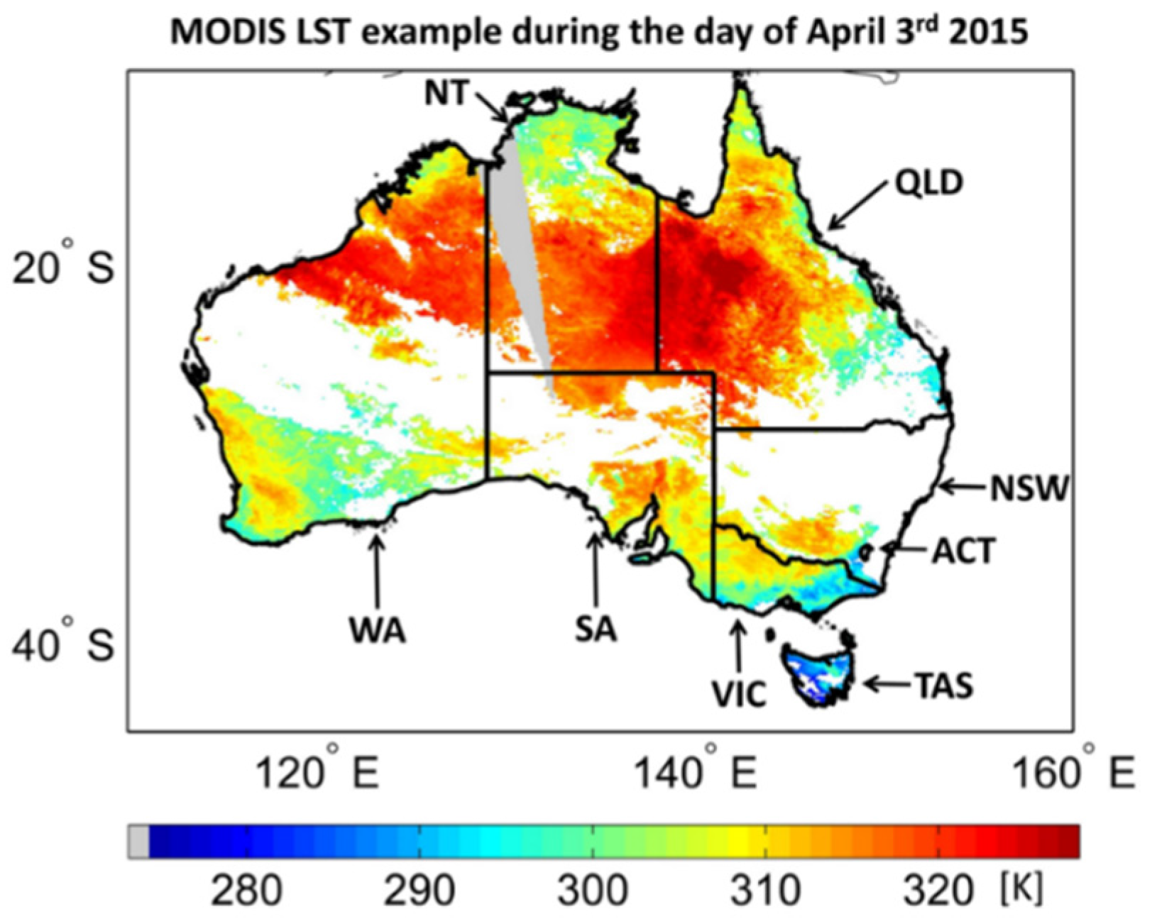
A further example of the individual MODIS and merged LST products was provides in Figure 8 and was, similar to Figure 1, based on observations made on 3 April 2015. Large parts of NSW, as well as significant parts of northeastern SA, southern QLD and TAS experience cloud cover on this day, hence the MODIS LST product (Figure 8a) presents no data values in these regions. These cloud gaps were filled by AMSR2 observations through the proposed combination approach resulting in an improved coverage over this part of Australia (Figure 8b). Figure 8c presents the spatial distribution of the sensors that were used in the combined LST product. Regions with gray shading are based on MODIS whereas the cyan regions are based on scaled AMSR2 observations.

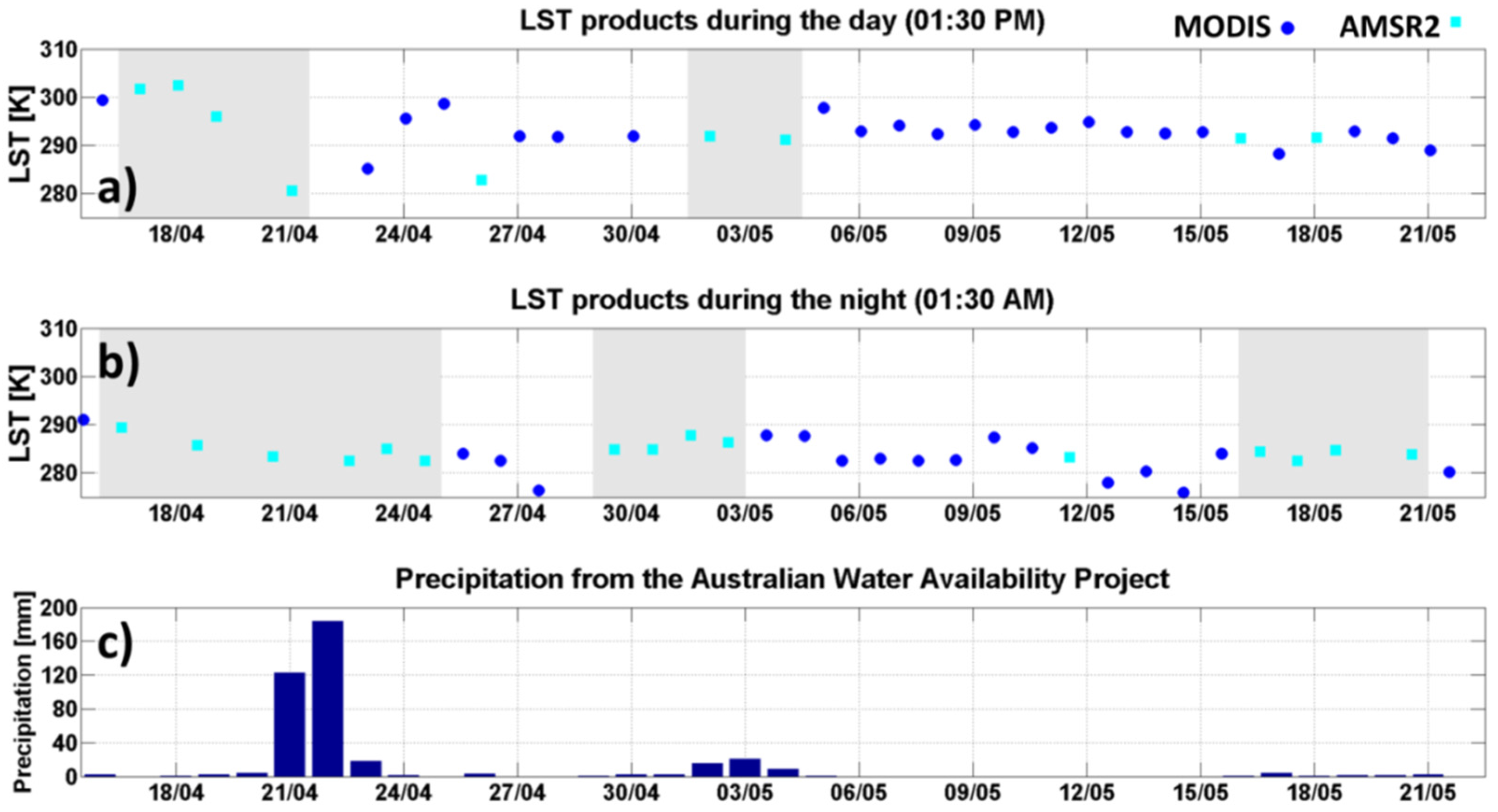
A final example that demonstrates the combination approach and its potential usefulness in operational systems was presented in Figure 9. Australia’s central coast received significant amounts of precipitation on 21 and 22 April 2015, which resulted in the Hunter Valley floods and was shown in Figure 9. This Figure 9c presents precipitation data for Maitland, a city located in the Lower Hunter Valley, for a five week period as obtained by the Australian Water Availability Project (AWAP; [17]. The AWAP precipitation shows roughly three separate precipitation periods of which the first resulted in significant floods. The obvious link between precipitation and cloud obstruction resulted in the absence of MODIS data during those precipitation periods. Those gaps in MODIS were then filled by AMSR2 observations as scaled through the proposed combination approach. The periods which heavily rely on these passive microwave observations were indicated through a grey background and demonstrate the successful scaling of AMSR2 observations resulting in an increasing number of LST observations.

4. Discussion

Areas in which disagreement was found between the MODIS and AMSR2 LST products could partially be related to known phenomena and differences between the day and night-time analysis could be related to the theory of thermal equilibrium. It should be emphasized that precipitation is generally associated with cloud cover leading to the absence of thermal infrared (TIR) observations towards the most critical time period in flood warning systems, which was the initial motivation for a pixel based scaling approach. The merged MODIS and AMSR2 product revealed a drop in performance compared to the individual products, the cost of a gain in revisit times. This performance drop was particularly visible in the tropical climate zone located in the north of Australia and can likely be attributed to higher uncertainties in the passive microwave products due to rain bearing clouds and active precipitation [18], as well as to higher uncertainties in the MERRA land surface model caused by convection processes [15]. Finally, it should be noted that AMSR2 LST retrievals in the merged products were only taken under cloudy conditions. Again, occasional rain bearing clouds or active precipitation may impact microwave emission, particularly when droplets are close to the size of the wavelength [18]. These phenomena could partially explain the performance drop of the merged LST product. In order to further understand the qualities of these individual and merged LST products, further quality assessment is needed. Techniques such as error propagation [19], radiance based validation studies, ground based validation studies or data assimilation techniques could serve as potential tools for this. Additionally, more sophisticated scaling approaches are likely to further improve obtained results as these can account for the impact of nonlinearities. However, it should be emphasized that the relatively simple linear regression performs well over the vast majority of the country. A potential approach to account for nonlinearities could be the replacement of the linear scaling by a polynomial regression approach. However, it should be noted that more sophisticated approaches could potentially hamper its usefulness in near real time application, a major advantage of the relatively simple approach proposed here.

5. Conclusions

A relatively simple combination approach that benefits from the cloud penetrating capacity of passive microwaves was presented. In a first step, the MODIS and AMSR2 LST products were compared and very high agreement was found over the vast majority of Australia. This agreement was found for the anomalies resulting in R² values generally ranging from 0.5 to 0.75 and for raw timeseries resulting in R² values generally ranging from 0.8 to 1.0. In a next step, pixel based scaling was proposed and the obtained results suggest that passive microwave observations from AMSR2 can successfully fill gaps caused by clouds or aerosol contamination in the MODIS LST product. By using AMSR2, the revised time increased on average by 20% but this varies per pixel as a result of the unique revised times of the satellite sensors as well as cloud and aerosol contamination. It should be emphasized that precipitation is generally associated with cloud cover leading to the absence of thermal infrared (TIR) observations towards the most critical time period in flood warning systems, which is most interesting in operational warning systems. The merged product also revealed a performance drop compared to the individual products which is the cost of a gain in revisit times. This performance drop was particularly visible in the tropical climate zone located in the north of Australia and can likely be attributed to higher uncertainties due to rain bearing clouds and active precipitation [18], as well as to higher uncertainties in the MERRA land surface model caused by convection processes [15]. The comparison against re-analysis data was subdivided over Australia’s major climate zones and revealed that the relative agreement between LST products against the re-analysis data is consistent over all these climate zones. It should be noted that our analysis was done for both raw time series as well as anomalies that better represent the interannual variability of the various products. In line with expectations, the relative performance of the anomalies drops when compared to the raw time series but overall findings were confirmed through both the anomalies and raw time series. Additionally, two examples were provided that demonstrate the proposed merging approach including an example for the Hunter Valley floods along Australia’s central coast that experienced significant flooding in April 2015.

References

1. Fang, B.; Lakshmi, V.; Bindlish, R.; Jackson, T.; Cosh, M.; Basara, J. Passive microwave soil moisture downscaling using vegetation and surface temperatures. Vadose Zone J. 2013. [Google Scholar] [CrossRef]
2. Fang, B.; Laskshmi, V. Soil moisture at watershed scale: Remote sensing techniques. J. Hydrol. 2014, 516, 258–272. [Google Scholar] [CrossRef]
3. Lakshmi, V. A simple surface temperature assimilation scheme for use in land surface models. Water Resour. Res. 2000, 36, 3687–3700. [Google Scholar] [CrossRef]
4. Parinussa, R.M.; Lakshmi, V.; Johnson, F.M.; Sharma, A. A new framework for monitoring flood inundation using readily available satellite data. Geophys. Res. Lett. 2016. in revision. [Google Scholar]
5. Wan, Z.; Li, Z.-L. A Physics-based algorithm for retrieving land-surface emissivity and temperature from EOS/MODIS data. IEEE Trans. Geosci. Remote Sens. 1997, 35, 980–996. [Google Scholar]
6. Bosilovich, M. A comparison of MODIS land surface temperature with in situ observations. Geophys. Res. Lett. 2006, 33, L20112. [Google Scholar] [CrossRef]
7. Parinussa, R.M.; Jeu, R.; Holmes, T.; Walker, J. Comparison of microwave and infrared land surface temperature products over the NAFE’ 06 research sites. IEEE Geosci. Remote Sens. Lett. 2008, 5, 783–787. [Google Scholar] [CrossRef]
8. Wan, Z.; Zhang, Y.; Zhang, Q.; Li, Z.-L. Validation of the land surface temperature products retrieved from TERRA moderate resolution imaging spectroradiometer data. Remote Sens. Environ. 2002, 83, 163–180. [Google Scholar] [CrossRef]
9. De Nijs, A.H.A.; Parinussa, R.M.; Jeu, R.A.M.; Schellekens, J.; Holmes, T.R.H. A methodology to determine radio frequency interference in AMSR2 observations. IEEE Trans. Geosci. Remote Sens. 2015, 53, 5147–5159. [Google Scholar] [CrossRef]
10. Holmes, T.; Jeu, R.; Owe, M.; Dolman, A. Land surface temperature from Ka-band passive microwave observations. J. Geophys. Res. Atmos. 2009, 114, D04113. [Google Scholar] [CrossRef]
11. Rienecker, M.; Suarez, M.; Gelaro, R.; Todling, R.; Bacmeister, J.; Liu, E.; Bosilovich, M.; Schubert, S.; Takacs, L.; Kim, G.; et al. MERRA—NASA’s modern-era retrospective analysis for research and applications. J. Clim. 2011, 24, 3624–3648. [Google Scholar] [CrossRef]
12. Scipal, K.; Holmes, T.R.H.; Jeu, R.A.M.; Naeimi, V.; Wagner, W. A possible solution for the problem of estimating the error structure of global soil moisture datasets. Geophys. Res. Lett. 2008, 35, L24403. [Google Scholar] [CrossRef]
13. Jeu, R.; Wagner, W.; Holmes, T.; Dolman, A.; Giesen, N.; Friesen, J. Global soil moisture patterns observed by space borne microwave radiometers and scatterometers. Surv. Geophys. 2008, 29, 399–420. [Google Scholar] [CrossRef]
14. Owe, M.; Jeu, R.; Holmes, T. Multisensor historical climatology of satellite-derived global land surface moisture. J. Geophys. Res. Earth Surf. 2008, 113. [Google Scholar] [CrossRef] [Green Version]
15. Taylor, C.; Jeu, R.A.M.; Guichard, F.; Haris, P.P.; Dorigo, W.A. Afternoon rain more likely over drier soils. Nature 2012, 489, 423–426. [Google Scholar] [CrossRef] [PubMed] [Green Version]
16. Peel, M.C.; Finlayson, B.L.; McMahon, T.A. Updated world map of the Köppen-Geiger climate classification. Hydrol. Earth Syst. Sci. 2007, 11, 1633–1644. [Google Scholar] [CrossRef]
17. Jones, D.; Wang, W.; Fawcett, R. High-quality spatial climate data-sets for Australia. Aust. Meteorol. Oceanogr. J. 2009, 58, 233–248. [Google Scholar]
18. Ulaby, F.T.; Moore, R.K.; Fung, A.K. Microwave Remote Sensing: Active and Passive; Artech House: Norwood, MA, USA, 1986. [Google Scholar]
19. Parinussa, R.M.; Meesters, A.; Liu, Y.; Dorigo, W.; Wagner, W.; Jeu, R. Error estimates for near real time satellite soil moisture as derived from the land parameter retrieval model. IEEE Geosci. Remote Sens. Lett. 2011, 8, 779–783. [Google Scholar] [CrossRef]
Figure 1. An example of the MODIS Land Surface Temperature product on 3 April 2015 (01:30 PM) that demonstrates cloud obstruction (e.g., WA, SA, NSW and ACT) which affects the availability of this Land Surface Temperature product. Note that the gray shading is an area that was not observed by the MODIS sensor on that particular day. Also, this figure presents the abbreviations for the Australian states that will be further used for reference purposes.
Remotesensing 08 00162 g001
Figure 2. The high agreement between the anomalies Land Surface Temperature products from MODIS and AMSR2 expressed in R2 (a) for day time observations; SE (b) for day time observations; R2 (c) for night time observations and SE (d) for night time observations.
Remotesensing 08 00162 g002
Figure 3. Histograms of the anomalies that show the agreement between the Land Surface Temperature products from MODIS and AMSR2 expressed in R2 (a) for day time observations, SE (b) for day time observations, R2 (c) for night time observations and SE (d) for night time observations.
Remotesensing 08 00162 g003
Figure 4. Pixel based scaling parameters (slope and offset) for MODIS Land Surface Temperature and AMSR2 (Tb, 37V) observations. The slope (a); offset (b) and the sample sizes (c) for day-time observations and the slope (d); offset (e) and the sample sizes (f) for night-time observations.
Remotesensing 08 00162 g004
Figure 5. R2 between the anomalies from MERRA and (a) MODIS; (b) the merged MODIS-AMSR2 Land Surface Temperature product and (c) AMSR2, as well as the percentage of gained samples through the addition of AMSR2 observations (d).
Remotesensing 08 00162 g005
Figure 6. Histograms that show the agreement between the anomalies from MERRA Land Surface Temperature and the remotely sensed Land Surface Temperature products from MODIS (a); AMSR2 (b) and through the presented combination approach (c) expressed in R2.
Remotesensing 08 00162 g006
Figure 7. Australia’s major climate zones according to the Köppen-Geiger climate classification. Several sub categories of the more detailed classification were merged into these four major classes.
Remotesensing 08 00162 g007
Figure 8. An example of the individual MODIS LST product for 3 April 2015 (a); the combined Land Surface Temperature product (b) and a spatial map (c) that demonstrates the sensors that were used in the combined Land Surface Temperature product. The Land Surface Temperature product in the gray shading is based on MODIS whereas the cyan regions are based on scaled AMSR2 observations.
Remotesensing 08 00162 g008
Figure 9. A recent flooding example for the Hunter Valley along Australia’s central coast demonstrating the combination approach and its usefulness for warning systems. This area experienced severe flooding after receiving significant amounts of precipitation on 21 and 22 April 2015. This timeseries demonstrates the successful scaling of AMSR2 observations resulting in an increasing number of Land Surface Temperture observations. (a) LST products during the day; (b) LST products during the night; (c) precipitation from the Australian Water Availability Project.
Remotesensing 08 00162 g009