Next Article in Journal
New Automated Method to Develop Geometrically Corrected Time Series of Brightness Temperatures from Historical AVHRR LAC Data
Next Article in Special Issue
Phylogenetic Structure of Foliar Spectral Traits in Tropical Forest Canopies
Previous Article in Journal
Mapping Plant Functional Types in Floodplain Wetlands: An Analysis of C-Band Polarimetric SAR Data from RADARSAT-2
Previous Article in Special Issue
Tree Species Abundance Predictions in a Tropical Agricultural Landscape with a Supervised Classification Model and Imbalanced Data
 
 
Erratum published on 12 May 2017, see Remote Sens. 2017, 9(5), 471.
Article

Automated Detection of Forest Gaps in Spruce Dominated Stands Using Canopy Height Models Derived from Stereo Aerial Imagery

by
Katarzyna Zielewska-Büttner
1,*,
Petra Adler
2,
Michaela Ehmann
1 and
Veronika Braunisch
1,3
1
Department of Forest Nature Conservation, Forest Research Institute Baden-Württemberg (FVA), Wonnhaldestr. 4, D-79100 Freiburg, Germany
2
Department of Biometry and Information Sciences, Forest Research Institute Baden-Württemberg (FVA), Wonnhaldestr. 4, D-79100 Freiburg, Germany
3
Conservation Biology, Institute of Ecology and Evolution, University of Bern, Baltzerstrasse 6, CH-3012 Bern, Switzerland
*
Author to whom correspondence should be addressed.
Submission received: 30 November 2015 / Revised: 29 January 2016 / Accepted: 9 February 2016 / Published: 25 February 2016
(This article belongs to the Special Issue Remote Sensing of Biodiversity)

Abstract

:
Forest gaps are important structural elements in forest ecology to which various conservation-relevant, photophilic species are associated. To automatically map forest gaps and detect their changes over time, we developed a method based on Digital Surface Models (DSM) derived from stereoscopic aerial imagery and a LiDAR-based Digital Elevation Model (LiDAR DEM). Gaps were detected and delineated in relation to height and cover of the surrounding forest comparing data from two public flight campaigns (2009 and 2012) in a 1023-ha model region in the Northern Black Forest, Southwest Germany. The method was evaluated using an independent validation dataset obtained by visual stereo-interpretation. Gaps were automatically detected with an overall accuracy of 0.90 (2009) and 0.82 (2012). However, a very high users’ accuracy of more than 0.95 (both years) was counterbalanced by a producer’s accuracy of 0.84 (2009) and 0.73 (2012) as some gaps were not automatically detected. Accuracy was mainly dependent on the shadow occurrence and height of the surrounding forest with producer’s accuracies dropping to 0.70 (2009) and 0.52 (2012) in high stands (>8 m tree height). As one important step in the workflow, the class of open forest, an important feature for many forest species, was delineated with a very good overall accuracy of 0.92 (both years) with uncertainties occurring mostly in areas with intermediate canopy cover. Presence of complete or partial shadow and geometric limitations of stereo image matching were identified as the main sources of errors in the method performance, suggesting that images with a higher overlap and resolution and ameliorated image-matching algorithms provide the greatest potential for improvement.

Graphical Abstract

1. Introduction

Structural complexity and niche diversity within forest habitats are important predictors for forest biodiversity [1,2,3]. Canopy cover [4], vertical variation of the canopy height [5] and forest gaps [6] are considered important structural elements in forest ecology to which various conservation relevant forest species are associated [7]. Presence or absence of many animal species such as European nightjar (Caprimulgus europaeus) [8], Capercaillie (Tetrao urogallus) [9], Grey-headed woodpecker (Picus canus) [10], various chiroptera [11,12,13], saproxylic beetles [14] or bird species assemblages [6,15] are expected to depend on semi-open forest habitats. Gaps in forest canopies also play a key role in various ecological processes such as the regeneration of trees and ground vegetation development, with the associated light regime being a main driver for composition and diversity of understory biota [16]. The establishment of an economically sustainable forest management with even-aged stands, as introduced by Hartig and Cotta in Europe at the beginning of 19th century [17], resulted in the simplification of the forest structure [18] and an underrepresentation of the early and late phases of the forest succession [19] that are characterized by a discontinuous canopy cover and the occurrence of forest gaps. The shift towards ecologically sustainable close-to nature forestry [20] has additionally led in recent decades in many European temperate forests to a progressive increase of growing stocks, with detrimental effects on many photophilic species. Species conservation programs and habitat restoration measures in temperate forests are therefore often directed towards the creation of canopy openings and gaps; yet this requires quantitative, taxon-specific information about the required size, shape, distribution and connectivity of gaps. To generate such information, to develop appropriate management strategies and to monitor their success, precise information on spatial distribution of organisms and on forest structures at relevant-often broad-spatial scales are necessary [21]. While such data were long missing, given the impossibility to derive area-wide mosaic-structures from plot-based forest inventories or the huge effort to visually assess and manually map such structures based on aerial photographs, the rapid development of remote sensing now offers the potential to deliver forest structural information across large spatial scales at an unprecedented degree of precision.
Size and spatial distribution are the most commonly mapped gap parameters for which various remote sensing data and techniques have been used [22]. Gap size and distribution pattern were mapped from satellite imagery by Garbarino et al. [23] and Hobi et al. [24]. Vepakomma [25,26] used Light Detection and Ranging (LiDAR) to assess spatial contiguity and continuity of canopy gaps over time in mixed wood boreal forests. Rugani et al. [27] based a similar research question using visual stereo interpretation of scanned color-infrared (CIR) aerial photographs. Getzin et al. [28] showed that very high-resolution images from unmanned aerial vehicles (UAV) can be used to effectively assess forest gaps and associated plant biodiversity in temperate forests. In recent years many studies confirmed the benefit from including forest structure parameters such as canopy cover and forest gaps derived from LiDAR into habitat models showing LiDAR to deliver precise, reproducible and high resolution information for answering a variety of ecological questions [5,6,15,29].
Despite the well-known, advantageous qualities of LiDAR and emerging possibilities of UAVs, digital aerial images currently represent the most cost-effective and accessible input data for operative forest remote sensing applications. Digital aerial images with large spatial coverage, consistent quality and a spatial resolution of 20 cm or less became standard products of regional mapping agencies in recent years [30,31,32,33]. Acquired in regular time intervals and available at relatively low costs, they are particularly interesting for forest monitoring and change-detection purposes.
Recent technical advances in the field of digital photogrammetry demonstrate the great potential of automatic image matching for deriving Digital Surface Models (DSMs) that can be used for an accurate characterization of the forest canopy structure [32]. Height measurements from the DSMs normalized versus DEM (nDSMs) also called canopy height models (CHMs) have been shown to perform very well when estimating timber volume or basal area on the plot, stand or country level [30,32,34] and might thus also be well suited for gap detection [34,35].
To map forest gaps and detect their changes over time in a cost-efficient way, we developed a method based on CHMs derived from stereo aerial imagery from public standard flight campaigns. We aimed for a gap mapping tool that would deliver reliable and replicable results when applied to available data either in form of original aerial imagery, point cloud or a raster DSM. One important scope thereby was to assess the viability of gap assessment based on publicly available, standard products of mapping agencies so as to evaluate their potential to deliver reliable forest structure information for monitoring programs at various spatial scales. Our method involves several steps: (1) the derivation of a CHM from stereo aerial imagery; (2) the quantification of canopy cover and height for pre-stratification; (3) the mapping of forest gaps and their changes; (4) the detection of gaps in specific locations (i.e., on forest roads); (5) the evaluation of the mapping accuracy; and finally (6) the identification of the main sources of error. In addition to the main aim, the mapping of forest gaps, the intermediate processing steps deliver other important forest structure parameters such as canopy cover and forest height diversity that are frequently required as predictor variables for species-habitat studies in forest ecosystems [36,37].

2. Material and Methods
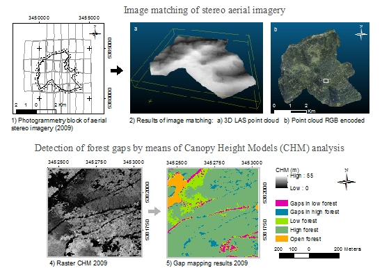
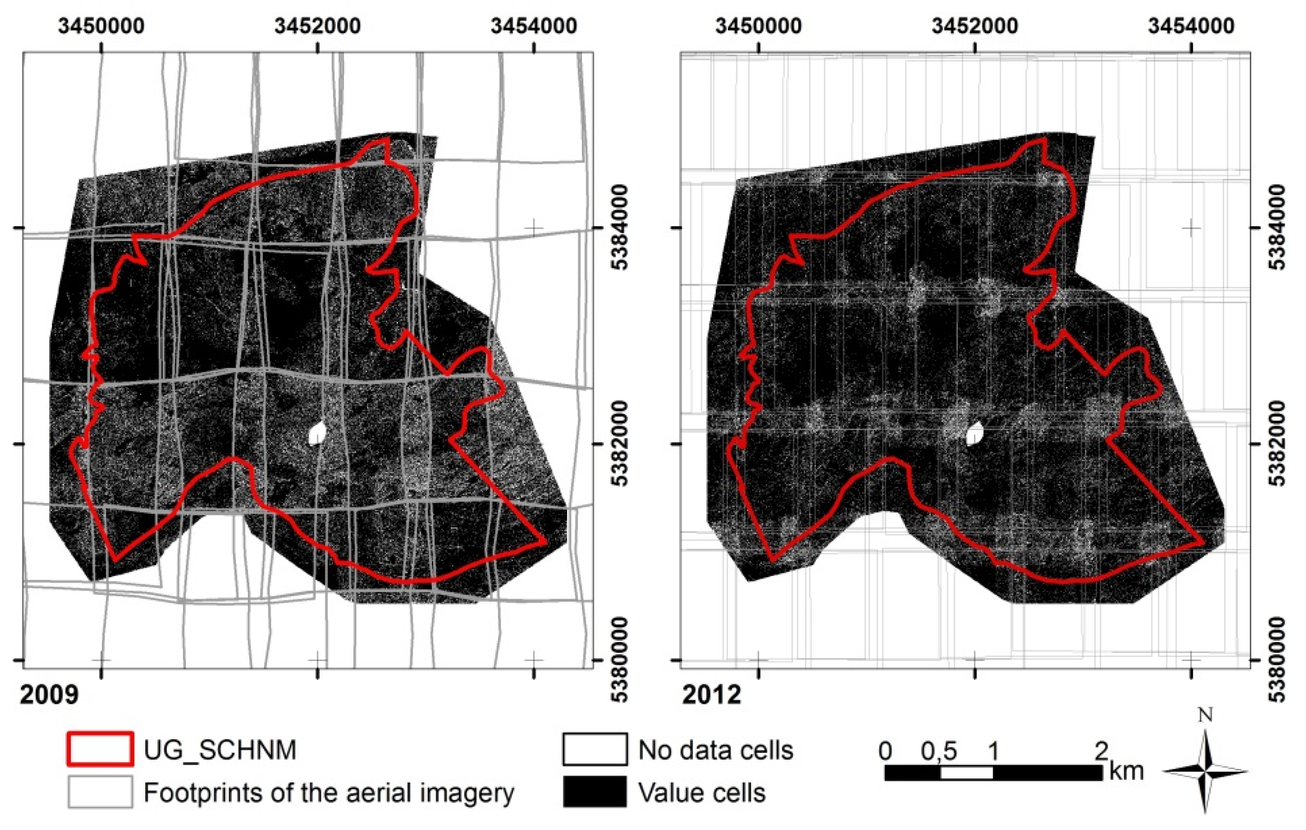
2.1. Study Area

The study area of 1023 ha is located in the State of Baden-Württemberg, Southwestern Germany, in the Northern Black Forest (8°34’E, 48°58’N). A lake covers 1.8 ha of the area, which reduces the effective study area to 1021.2 ha. The area was chosen due to its high diversity with regard to topography, forest successional stage, protection status and consequential different management regime.
The elevation within the study area ranges from 493 to 941 m. According to the classification of the AG Boden [38] most slopes (77.5%) are very steep (>20°) or strongly inclined (10°–20°). The Northern Black Forest belongs to the most forested regions in the state of Baden-Württemberg (forest cover of 69% [39]) and has been used for litter and timber extraction over centuries [40,41]. The dominant tree species is Norway spruce (Picea abies L.) with admixture of Silver fir (Abies alba Mill.) and Scots pine (Pinus sylvestris). In 82% of the forest stands, the broadleaves tree species account for less than 30%. In addition, the area is characterized by a dense forest road network of 187 m/ha (19 km in total).
At the time of the acquisition of the aerial photographs used for this study (2009 and 2012), the southern part of the study area was protected according to the European law as a NATURA 2000 site (391.6 ha) completely overlapping with a forest reserve managed for conservation purposes (172.7 ha).

2.2. Material

2.2.1. Aerial Imagery

As a primary input data, two aerial imagery data sets from the two flight campaigns, of 2009 and 2012, were used (Figure 1, Table 1). The data (including the absolute orientation of the images) were provided by the state agency of spatial information and rural development of Baden-Württemberg (LGL) with 4 channels (red, green, blue and near-infrared (RGBI)) and radiometric resolution of 8 (2009) and 16 (2012) bit. The overall spatial resolution of the imagery was 20 cm with an overlap of 60% (end lap) and 30% (side lap).

2.2.2. Additional Data Sources

In line with our goal of using only publicly available data, we also limited the additional data sources to the products of the LGL or internal data of the forestry administration. A DEM with 1 m resolution (DEM01) derived from LiDAR-data [42] was used as a ground surface for the generation of the CHMs. Slope and aspect were derived from a DEM with 50 m resolution (DEM50) [42]. In addition, for identifying gaps along or influenced by forest roads, we used the forest road network datasets of the State Authority Topographical and Cartographical Information System (ATKIS) [43] and the Department of Forest Geoinformation of Baden-Württemberg [44].

2.3. Methods

2.3.1. Forest Gap Definition

In the literature, there are inconsistencies with regard to terminology, methods for gap identification and modeling gap dynamics [45]. Two main definitions of forest gaps can be found. The first defines a canopy gap as a “hole” in the forest canopy cover down to a predefined height (e.g., 2 m) above ground [46]. According to the second definition, the gap additionally includes the ground surface below the canopy extending to the base of the trees which surround the canopy opening [47]. Definitions also vary depending on the assessment method and research objective: A terrestrial “bottom-up” approach, mostly used in field surveys [46] predefines a fixed maximum vegetation height within the gap while the aerial “top-down” approach considers in the first place the technical capabilities of the sensor penetration through the tree canopy to forest ground and therefore defines a maximum vegetation height in a gap in relation to the height of the surrounding trees [48,49]. Often, the gap is passively mapped as the area remaining between the actively mapped trees.
The definition used in this study was based on a combination of the above mentioned definitions: We define forest gap as a canopy opening of at least 10 m2 in dense forest (≥60% canopy cover) reaching through all forest strata down to maximum 2 m vegetation height in high forest stands (≥8 m height) and down to maximum 1 m in low forest stands (<8 m height).
We considered a minimum stand size of 0.3 ha, which corresponds to the conventional minimum stand size in Baden-Württemberg [44]. Areas with canopy cover less than 60% and exceeding 0.5 ha were classified in line with Ahrens et al. [50] as “open forest”. Open spaces within this forest type were considered as inherent stand characteristic and thus not mapped as gaps. The minimum size of a gap was set to 10 m2 according to Müller and Wagner [51] and Schliemann and Bockheim [45]. The maximum gap-vegetation height of 2 m was chosen compliant with Brokaw [46] and adapted to 1 m in the lower stands after the first mapping tests, which revealed that gaps within the lower stands were not significantly distinct when using the 2 m threshold.

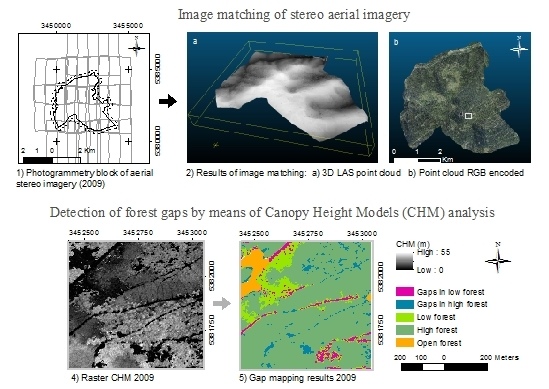
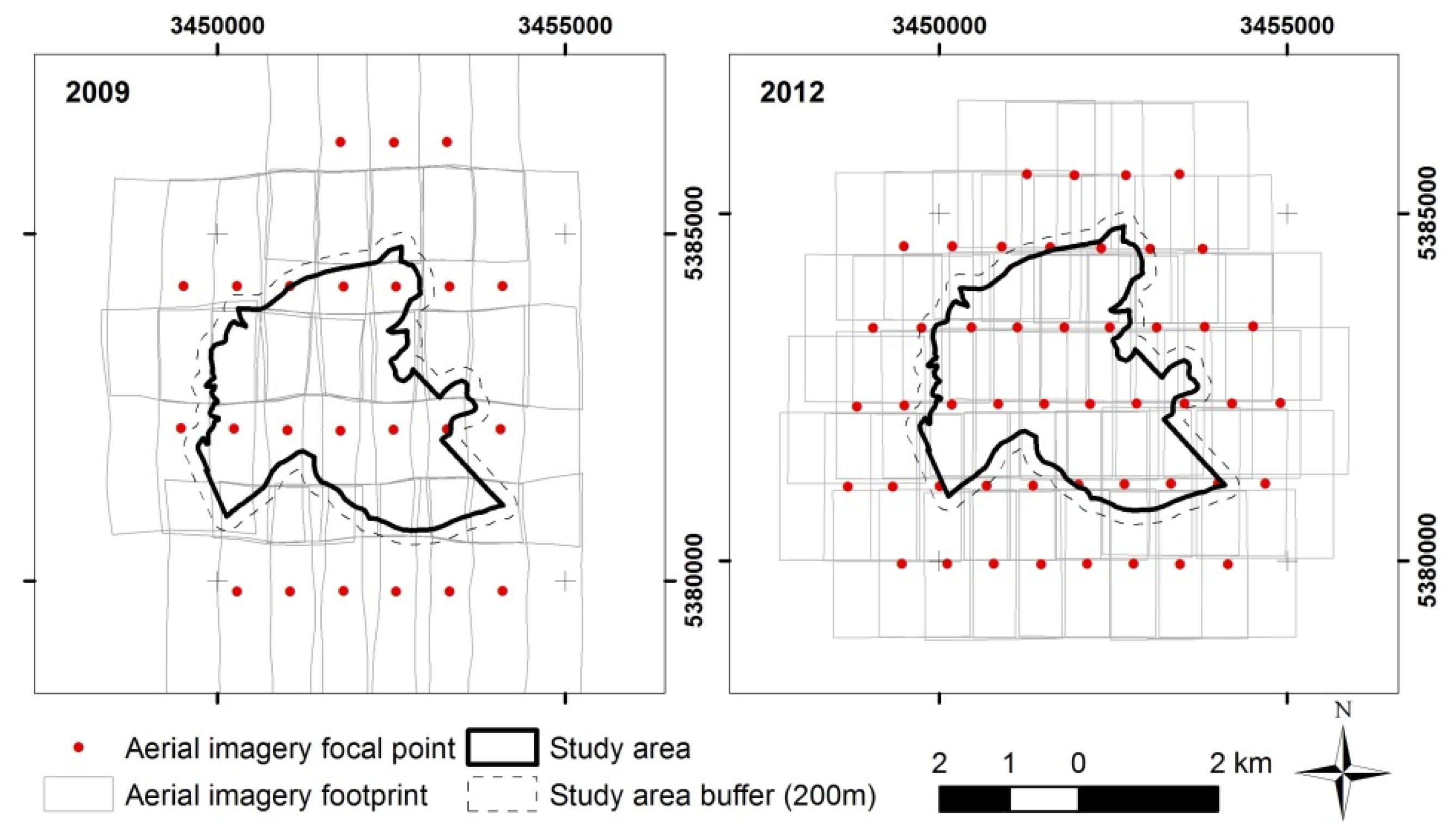
2.3.2. Calculation of Canopy Height Models (CHM)
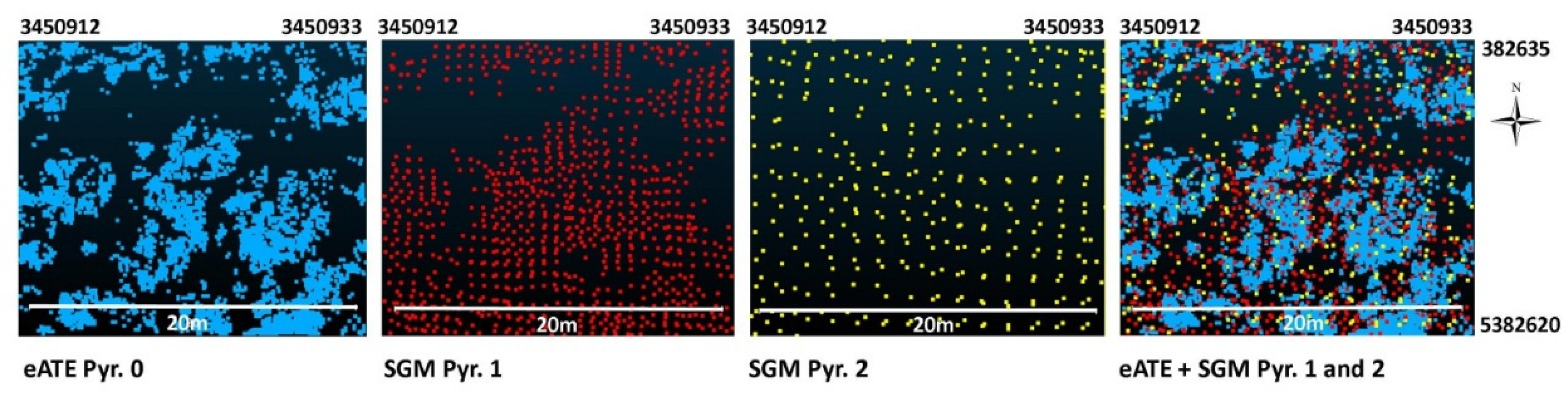
Canopy Height Models were generated in two steps: (1) image matching and (2) point cloud processing (Figure 2).

Image Matching

DSMs with a spatial resolution of 1 m were calculated from the stereo imagery. To avoid artifacts at the borders of the study area, both during the image matching process and during the subsequent raster analysis using a moving window, the study area was buffered with 200 m. For each study year, two point clouds were generated using Leica Photogrammetry Suite enhanced Automatic Terrain Extraction (LPS eATE [52]) and Semi Global Matching (SGM XPro [53]) algorithms. Both algorithms returned different point clouds partially complementing each other (Figure 3).
Image matching for terrain extraction result in a first step in an irregular point cloud depending on the algorithm, site conditions and camera properties and situation [54]. Consequently, not every cell of a DSM raster is covered by a matched point and the generated DSMs consist of a certain percentage of cells without original height information (“no-data” cells).
The input pyramid layer was identified as one of the key factors affecting point density and distribution of the generated point cloud. It also influences the point resolution and accuracy as the coarser (higher) image level delivers points with lower accuracy, especially in situations of irregular canopy surface. Based on visual assessment, we decided for a combination of 3 point clouds from eATE and SGM processed with the pyramid levels 0, 1 and 2, respectively, which provided good point coverage in reasonable processing time. The detailed settings of both algorithms are listed in Table 2.

Point Cloud Processing

In the next processing step only LAS points between −1 and 55 m height in relation to the DEM01 point cloud filtered with LAStools [55] were retained, which removed most of the outliers and resulted in the normalized land cover surface heights (Figure 2). The “LasDataset to Raster” transformation (Data Management Toolbox in ArcGIS) with the inverse difference weighting (IDW) for interpolation and the natural neighbor void fill method was applied to calculate CHMs with a 1 m resolution as a basis for subsequent height analysis and forest gaps extraction.

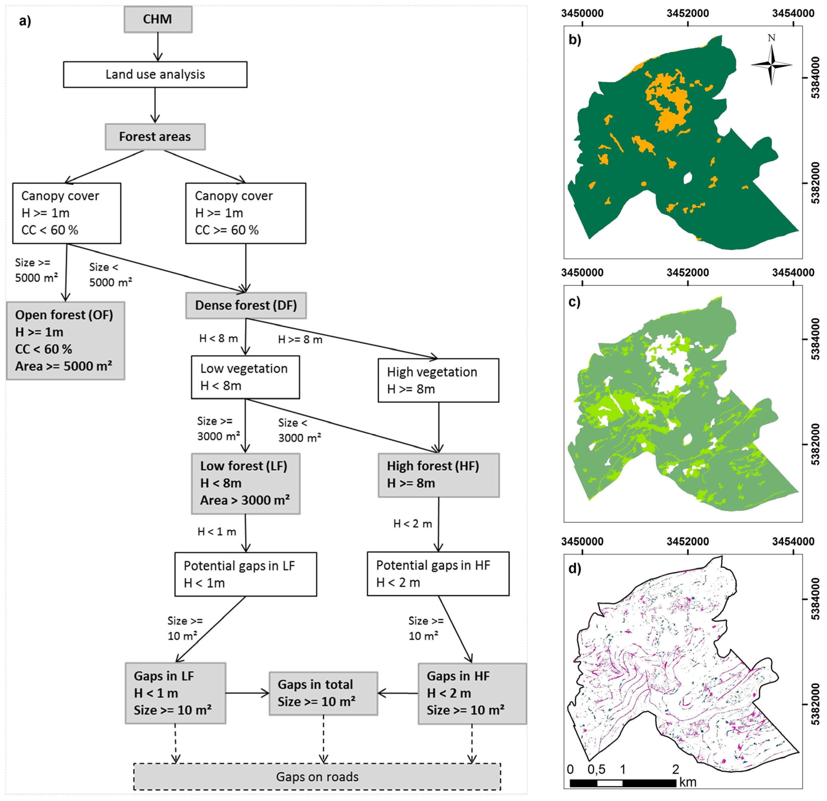
2.3.3. Gap Extraction

Forest gap extraction based on the CHM was performed in ArcGIS 10.3 [56] (raster and vector based) in three steps (Figure 4): (1) identification of open and dense forest; (2) classification of dense forest into height classes of low and high forest; and (3) gap extraction in the latter two classes. In an additional post-processing step (4) gaps on and next to forest roads were located.

Open and Dense Forest

In the first step of the object based raster analysis (Figure 4a), open (OF) and dense forest (DF) areas were identified based on the CHM (Figure 4b). Based on the proportion of vegetation higher than 1 m within a circular moving window (r = 25 m), directly adjacent neighboring cells with values of canopy cover percentage (CC) of 60% or less were aggregated (Spatial Analyst function: region group, 4 neighbors) to open forest patches when aggregations were greater than 0.5 ha. The remaining cells representing either gaps or dense forest were submitted to further gap extraction.

Low and High Stands

Within dense forest, cells with CHM-values <8 m were identified and grouped (region group, 4 neighbors) into low forest (LF) stands, when their size exceeded 0.3 ha (Figure 4c). The remaining cells were classified as high forest (HF).

Forest Gaps

Forest gaps were identified separately for LF and HF (Figure 4d). All cells with canopy heights less than 1 m within LF were identified and grouped using the function region group with 8 neighbors, i.e., including neighboring cells with adjacent border as well as diagonal neighbors. The same procedure was carried out for raster cells less than 2 m height within HF. In both classes, LF and HF, groups with a minimum size of 10 m2 were retained and reclassified into forest gaps.

Gaps on and Next to Forest Roads
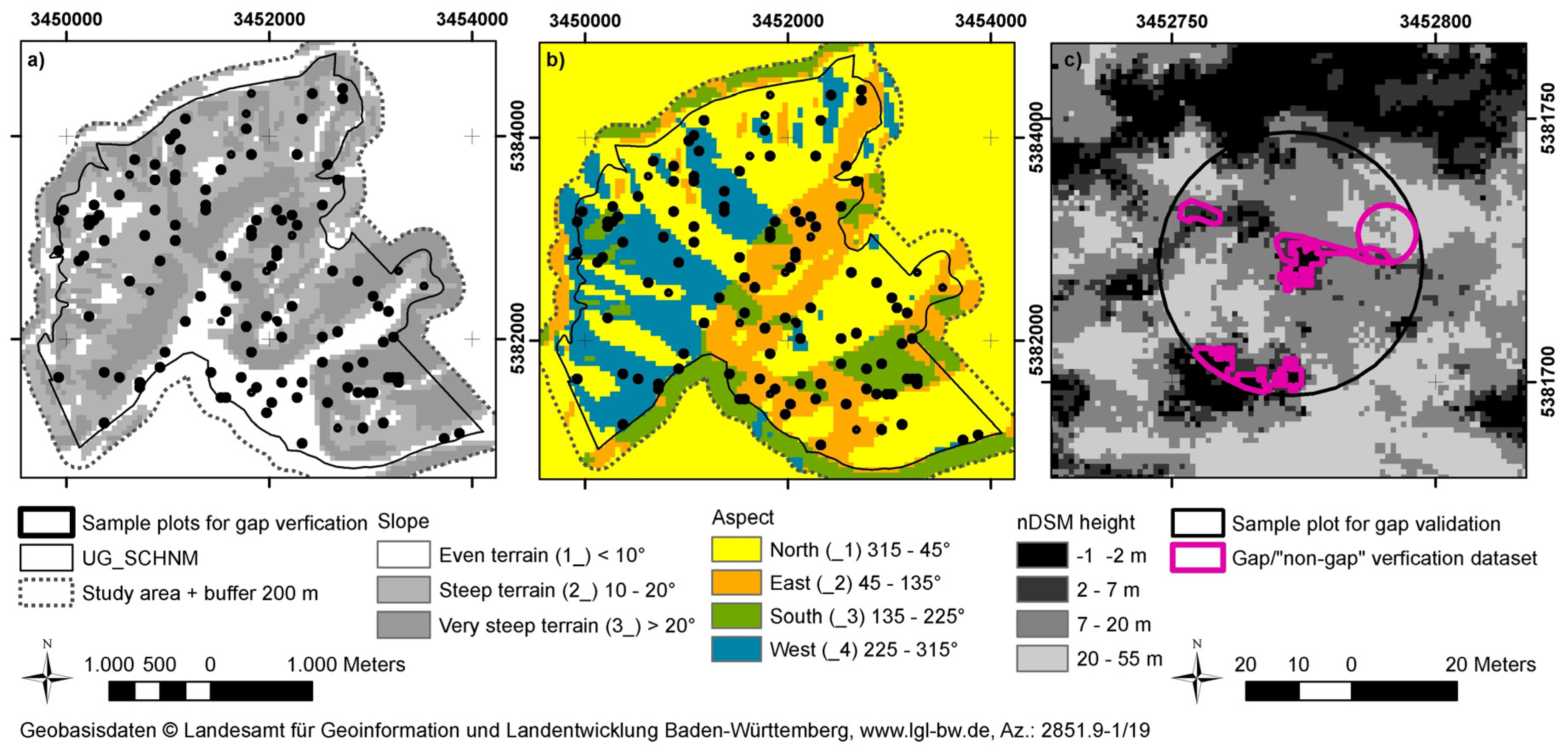
Gaps on and next to forest roads and skidding trails were identified in a post-processing step using 2D reference vector data from ATKIS and Forest Geoinformation databases. Since both files contained minor errors (i.e., missing data and location inaccuracies) features missing in the more comprehensive ATKIS file were added from the Forest Geoinformation database. Gaps located on or adjacent to roads were selected within a 5 m buffer to both sides of the road or skidding trail (Figure S1).

2.3.4. Validation

The discrimination between open and dense forest and the detection of gaps were evaluated by a comparison with visual stereo-interpretation of the original aerial imagery using Stereo Analyst for ArcGIS 10.2 [57]. Therefore we generated independent evaluation data at circular sampling plots (r = 25 m, corresponding to the window-size used for open and dense forest classification). Two sets of evaluation plots were generated. For testing the accuracy of the classification into open and dense forest an equal amount of plots was placed randomly in both forest types. The plots for evaluating the performance of the forest-gap detection were selected according to a stratified random design.

Open-Dense Forest

For evaluating the accuracy of the classification into open and dense forest 40 plots were randomly placed in each of the two classes (Figure 5a). With a plot size of 1962.5 m2, the total evaluation area per class amounted to 7.9 ha, corresponding to 9.5% and 27.0% of the open forest of 2009 and 2012 respectively. A change of the forest type from open to dense between 2009 and 2012 was allowed for additional validation of the change-recognition performance. The set of sample plots located in open forest of 2009 was therefore also kept in 2012. However, since 30 of the evaluation plots in the open forest changed to dense forest in 2012 additional 30 sample plots were generated within the open forest of this year to maintain a balanced verification dataset. Within the evaluation plots canopy cover was visually estimated in 5% steps, aided by schematic illustrations [50,58], and the forest class was assigned accordingly. The agreement between visual and automatic mapping was assessed using different evaluation indices based on a confusion matrix. Overall, producer’s (probability that the automatically mapped class was also visually confirmed) and user’s [59] (probability that visually interpreted class was also automatically classified as such) accuracy [60,61,62] as well as Cohen’s kappa [63] were calculated using the package “caret” in R [64].

Gaps

Since the gap-mapping accuracy was expected to vary in relation to two terrain parameters, slope and aspect, evaluation plots were stratified along these two gradients: Three classes of slope (0°–10° plane, 10°–20° strong inclined or steep, and >20° very steep, according to the definition of AG Boden [38] and in line with Wrbka et al. [65]) and 4 classes of aspect (north 315°–45°, east 45°–135°, south 135°–225°, and west 225°–315°) resulted in 12 terrain situations that were extracted from the DEM50 (Figure 5a,b). The focal point of each 50 m × 50 m cell represented a possible center of an evaluation plot (r = 25 m).
Forest gaps were evaluated on 120 evaluation plots (10 per terrain stratum) (Figure 5a,b) covering a total area of 23.6 ha, which corresponds to 2.4% of the dense forest in each study year. Within the evaluation plots gaps with an area of at least 10 m2 inside the plot (168 in 2009 and 171 in 2012) were visually assessed, delineated and (Figure 5c) compared with the automatically mapped gaps located with at least 10 m2 inside the evaluation plot. To assess the correct classification of gap–absence, we placed circles in the dense forest areas within the sampling plots in size corresponding to the mean size of the visually verified gaps (95 m2 in both years) (Figure 5c). The total number of circles randomly distributed among the sampling plots was equal to the total number of the visually verified gaps.
Correct agreement between visually and automatically mapped gaps was assigned if there was an overlap of at least 80%. “Non-gap” circles were attributed as “wrongly classified” when a gap of at least 8 m2 (80% of the minimum gap size) was identified within it. The agreement between visual and automatic mapping was again assessed by means of overall, producers’ and users’ accuracy and Cohen’s Kappa.

Variables Affecting Mapping Accuracy

Since we expected the accuracy of the method to be affected by external factors, selected characteristics of the viewed gaps were visually assessed for each of the gaps mapped in the evaluation plots (Table 3). Effects of the recorded variables such as gap size, height of the surrounding forest, presence of shadow, slope, aspect and gap location were tested using Conditional Inference Trees (ctree) vignette of R-package “partykit” [66,67].
We also evaluated whether missing information in some raster cells (“no-data” cells) could be a reason for a fraction of the undetected gaps. In a DSM created from an eATE point cloud “no-data” cells amounted to 10%–15% whereas in a DSM generated from the SGM point cloud this percentage was much lower (2%–3%). This difference was caused by an internal interpolation used by the SGM algorithm during the matching process resulting in an artificial assignment of values to cells, where no points were directly matched.

3. Results

3.1. Mapping of Open and Dense Forest

Mapping of open forest areas resulted in 82.7 ha (8% of the study area) and 28.8 ha (3%) in 2009 and 2012, respectively. The number of open forest patches decreased from 31 to 28. This includes also open forest patches smaller than 0.5 ha located at the border of the study area but being part of larger open forest areas. The mean size of the open forest patches within the study area changed from 3.5 ha to 1.6 ha, which illustrates the closure of open forest areas from their borders inwards. Dense forest amounted to 938.5 ha (92% of the study area) in 2009 and 992.5 ha (97%) in 2012.
The classification obtained with the chosen settings agreed well with the results of the visual assessment (Table 4, Figure S2, Table S3) with accuracy measures between 0.85 and 1.00 confirming a very good performance of the method. An assessment of the 12 erroneous classifications revealed that deviations between automatic and visual estimation occurred in plots with canopy cover estimates ranging between 30% and 80%, with most (75%) of the errors occurring within a narrow 10% buffer (50%–70%) around the canopy cover threshold of 60%. In nine of the 12 cases, the automated method overestimated the canopy cover. An increased rate of deviation (20%) was found in the 30 plots that changed from open forest in 2009 to dense forest in 2012, which confirms that areas with canopy cover close to the threshold are particularly prone to misclassification.

3.2. Identification of Low and High Forest

Patches with low (LF) and high (HF) forest amounted to 82 (175.0 ha) and 18 (763.6 ha), respectively, in 2009, versus 70 (211.3 ha) and 22 (781.3 ha) in 2012 (Table S4). Within the dense forest, high forest stands dominated with a share of about 80% forming large compact patches with a mean size of 42.4 ha (2009) and 35.5 ha (2012). The total area of both low and high dense forest increased from 2009 to 2012 to the disadvantage of the open forest. Low stands-on average much smaller than high stands-got consolidated and increased significantly in area and size, from a mean size of 1.8 ha in 2009 to 2.9 ha in 2012.

3.3. Forest Gaps Mapping

The automated mapping approach detected 4575 (2009) and 4667 (2012) gaps in the dense forest. Total gap density was 4.9 gaps per ha (7.2% of the dense forest area) in 2009 and 4.7 gaps per ha (6.3%) in 2012 (Table S5). Generally, many more (13.7–14.6 N/ha) gaps were mapped in the low forest than in the high forest (2.0–2.8 N/ha).

3.3.1. Mapping Accuracy

The comparison of automatic gap-detection with the visually identified gaps revealed good agreement (Table 5 and Table 6) with an overall accuracy of 0.90 and 0.82 in 2009 and 2012, respectively, and corresponding Kappa values of 0.80 and 0.66. User’s accuracies greater than 0.96 show that almost all automatically detected gaps were correctly classified. However, a fraction of the visually identified gaps were not captured during the automated mapping process, which is reflected in omission errors of 0.16 (2009) and 0.28 (2012). Method performance for the “non-gap” areas showed an opposite pattern with producer’s accuracies greater than user’s accuracies.
However, 71% (2009) and 73% (2012) of the visually but not automatically identified gaps were adjacent to automatically mapped gaps indicating that a significant proportion of the gaps have been captured correctly, but the extent delineated was too small.

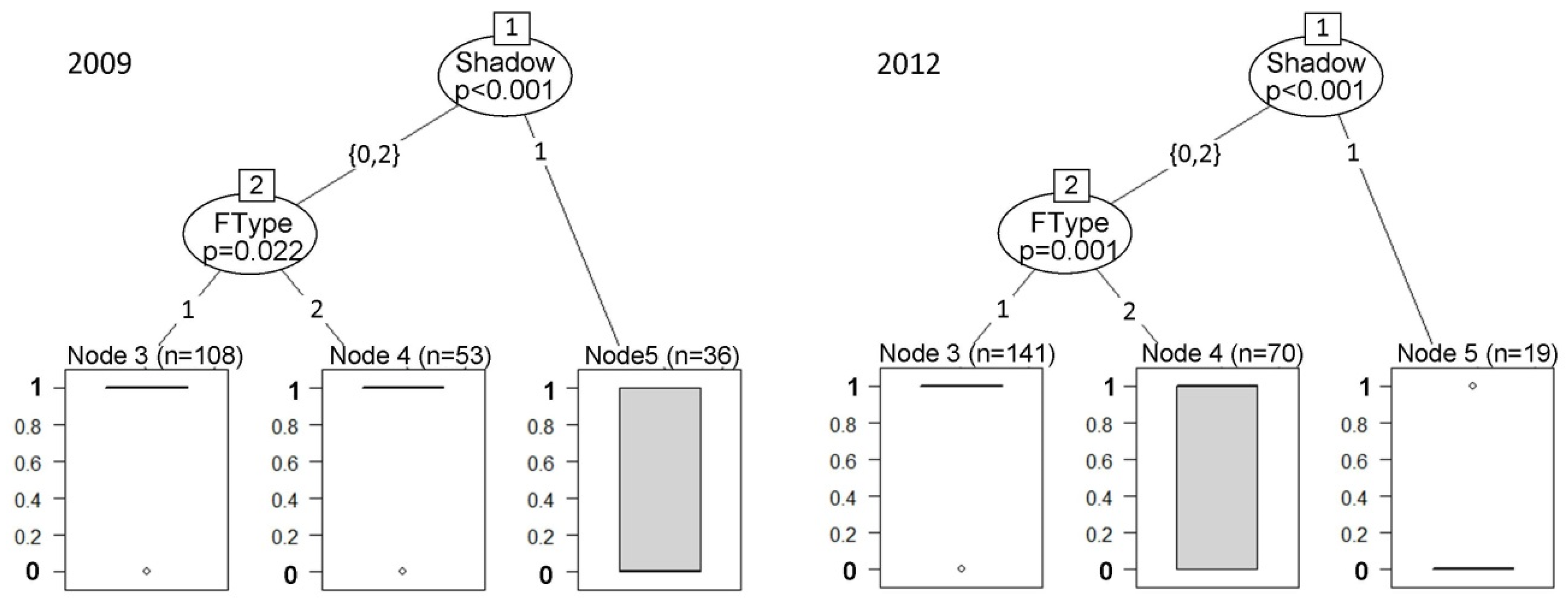
3.3.2. Variables Affecting Mapping Accuracy

Among the tested variables, shadow occurrence and forest height class affected mapping accuracy (Figure 6), while no significant effect was found in relation to the other variables tested (Table 3). Presence of shadow strongly limits the penetrability of an optical sensor into the lower parts of the canopy. In both study years, the occurrence of full shadow in the incision in the forest canopy was the main cause for the erroneous delineation of gaps. The effect of shadow was also confirmed directly during visual verification, as the most of the visually identified but not automatically mapped gaps (70%–87%) were identified in areas of total or partial shadow (Table S6).
The height of the surrounding forest stand (LF and HF) determining the depth in the canopy, to which the light can penetrate, is also strongly linked to shadow occurrence. While in 2012 the height of the surrounding forest caused increased failure in gap mapping in HF, in 2009 this tendency was not pronounced. Generally, the gaps in locations without or with partial shadow occurrence were mapped with a high accuracy in LF and less reliability in HF, whereas the complete shadow occurrence hinders the gap mapping performance in all stand types.
Despite similarly user’s accuracies of 0.96–0.98 and overall accuracies higher than 0.79, producer’s accuracy in high forest was much lower than in low forest with 0.70 in 2009 and 0.52 in 2012 (Table 7 and Table 8).
The analysis of the “no-data” cells revealed that they did not only occur in shadowy incisions in the canopy cover, e.g., along roads or in stands with a highly heterogeneous vertical structure but also in low forest stands and on hilltops where aerial photographs should theoretically deliver good material. Such “no-data” cells were mostly located along flight strips (2009), particularly in the outer parts of the lateral and longitudinal overlapping zone of the images (2009 and 2012) (Figure 7).
An intersection of the “no-data” layer with the gap validation dataset showed that only ca. 10% cells of all visually, but not automatically identified gaps were actually classified as “no-data” cells (Table S7). The assignement of new values to original no-data cells by means of interpolation from the neighbouring points during the image matching or raster transformation resulted in height values depending on the surrounding forest characteristics.

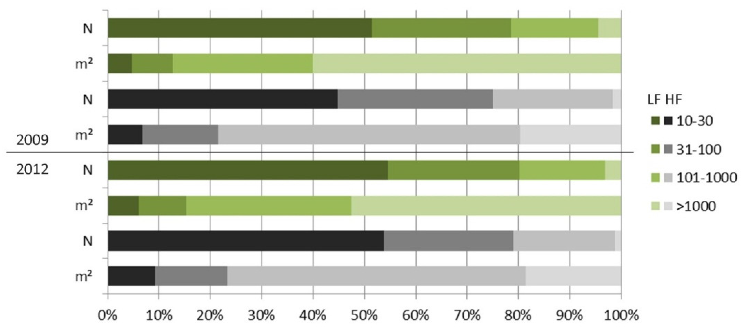
3.3.3. Gap Size and Total Area
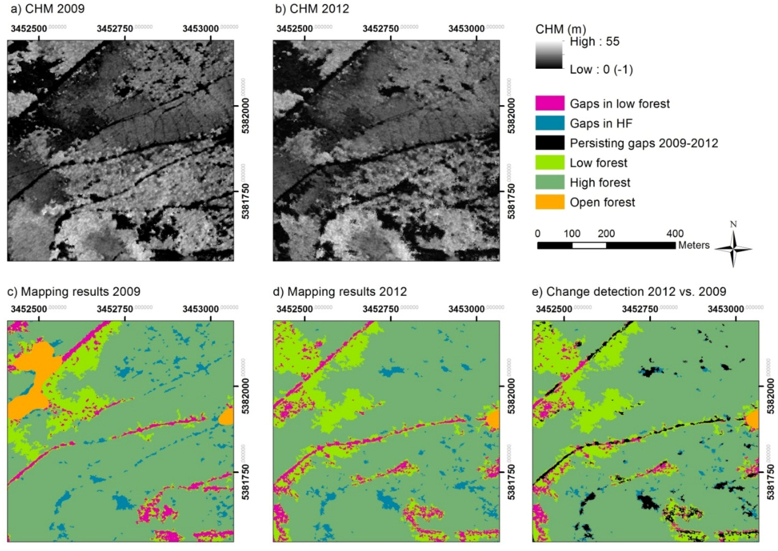
In the study area, gap sizes ranged from 10 m2 (predefined minimum size) to 19,091 m2 and 12,556 m2 in low forest (2009 and 2012, respectively) and to 2105 and 2495 m2 in high forest (Table S5). Despite the great difference in maximum sizes, median values ranged between 26 and 36 m2. In 2009, gap size was significantly greater in LF than in HF (Wilcoxon rank sum test, p-value = 0.0006), whereas in 2012 this characteristic was no longer pronounced (p-value = 0.5644).
The most and the largest gaps were mapped in low stands, even though they constituted only about 20% of the dense forest in both years. Moreover, the variance in gap size was most pronounced in LF, with standard deviations 2.5–3.2 times larger than for gaps in HF in the same study year. In high forest, number, mean size, median size and density of the gaps decreased between 2009 and 2012 amounting to a 36% reduction of the total gap area in this class. In contrast, the amount and density of gaps in low forest increased from 13.8 gaps per ha in 2009 to 14.6 gaps per ha in 2012, with only minor increase of the total area.
Most gaps mapped in both stand types were very small (10–30 m2) or small (31–100 m2), together making up 75%–81% of all gaps and 13%–23% of the total gap area in all height classes and years (Figure 8). In low stands the greatest fraction of the total gap area (53%–60%) consisted of very large gaps (>1000 m2), whereas in high stands 58%–59% pertained to large gaps (101–1000 m2). In both low and high forest the number and area of smaller gaps increased, whereas the large and very large gaps decreased from 2009 to 2012.

3.3.4. Gap Changes

55% of the gaps recorded in low stands and 30% of the gaps in high stands mapped in 2009 were also confirmed in 2012 (Table S5, Persisting gaps 2009–2012, Figure 9). A substantial proportion (37% of N, 45% of the total area) of gaps found in low forest in 2012 originated from open forest in 2009. Shifts between low and high forest were not that significant with 17% of gaps in high forest of 2012 originating from gaps in low stands of 2009. The remaining differences in the amount of mapped gaps between the study years were due to displacement or shrinking of gaps.

3.3.5. Gaps on Forest Roads

Within the evaluation plots, 60 (30%) gaps in 2009 and 85 (36%) in 2012 were identified directly on a road or skidding trail, another 18 (9%) and 17 (7%) were found adjacent to these distinct linear features (Table S8).
These figures were slightly higher than in the total study area where—depending on the mapping year and forest height class—37% (2009) and 25% (2012) were located on or adjacent to a forest road (Table S9). Even though not all these gaps were captured due to shadow occurrence and canopy closure above the road (Figure S1), this gap type represented 67%–80% of the total gap area each year and forest height class, with an average gap-size varying from 40 to 88 m2.
Excluding the gaps on or next to roads resulted in an average gap density of 10–11 gaps/ha in LF and 1–2 gaps/ha in HF and average gap-size of about 50 m2 (Table S10).

4. Discussion

Assessing forest gaps for biodiversity research purposes requires a clear definition and classification of gaps in relation to the research goal. The definition we adopted adhered to the fact that most species-habitat studies refer to gaps as canopy openings with a fixed maximum height of vegetation in a gap. Given the great variance in species-specific requirements regarding forms and types of gaps and in order to maintain a broad applicability for habitat assessments for various species, we applied a low threshold regarding minimum gap size and no a priori restrictions regarding shape or minimum diameter. With regard to gap-delineation based on remote-sensing this definition entails some general limitations which are related to the penetrability of the light through the tree canopy. In addition, compared to using LiDAR-based assessments, specific problems arise when using aerial imagery for deriving measures of vegetation height as a basis for gap-delineation.

4.1. Image Matching and Canopy Height Models

Regularly updated and standardized aerial photographs from public flight mapping campaigns offer good possibilities for assessing forest structure in a cost-efficient way, especially when aiming at long-term monitoring. Primarily acquired to deliver high accuracy 3D earth surface measurements for general administration, economy and science applications these data-offered for public research at a special low cost-also provide a valid basis for mapping forest gaps with high accuracy. Even so, the image matching algorithms using aerial and satellite imagery for deriving DSMs still bear some potential for improvement, especially in rugged terrain and forest stands of complex structure [24]. Wang et al. [33] indicate that their method provides a high degree of accuracy in managed mixed forest, with lower accuracies in mountainous forests, which can be explained by the mismatch between the generated DSMs as a result of different flight angles of the imagery from different flight campaigns. Similar situations can be observed in our study, due to the acquisition of the aerial imagery in different study years, where the data provider used two different cameras. Adler et al. [54] observed that even in flat terrain different DSM matching algorithms produce different results, especially in highly structured canopy situations. Mountainous forests are likely more structured than intensively managed stands in the lowlands and thus particularly prone to shadow occurrence. In our study most of slopes were steep or very steep which definitely influenced the quality of the aerial imagery and the DSM accuracy.
The distribution of “no-data” cells points towards multiple sources of problems: first, inaccurate point matching in the outer areas of the camera viewing angle, second, shadow occurrence and third a possible inaccurate relative orientation of the stereo images.
The use of a “terrestrial bottom-up” gap-definition with predefined fixed (in contrast to a relative) maximum gap-vegetation height entails a significant effect of the DSM quality on the gap mapping performance, as inaccuracies in the surface heights in the order of magnitude of 1 m or more [30,68] significantly affect the delimitation of gaps with a maximum ground vegetation heights of 1 or 2 m.
Since the user’s influence on the acquisition process and quality of aerial imagery from standard flight campaigns of national or regional mapping agencies is limited, some shadows have to be accepted [33]. However, it is crucial to know the accuracy of the input data as they influence the usability and reliability of the generated DSM [68]. A quality assessment of the aerial imagery concerning light conditions and associated shadow occurrence could thus be beneficial. In our study, the details regarding flight time of acquisition of the aerial images were not available.

4.2. Forest Classification and Gap Identification

DSMs derived from aerial imagery proved promising for forest gap identification as the results of canopy cover and forest gaps mapping were good, Moreover, important for application across large areas, gap extraction from a ready CHM was very fast (i.e., 170–250 ha per minute, depending on processor and memory), whereas the image matching was the most time-consuming part.
As one crucial step in the workflow the class of open forest was delineated. This is an important feature for many forest species and therefore a valuable side-product of our study. Canopy cover estimation both in entirely open areas as well as in a mixture of open and dense forest stands worked well, with uncertainties mostly occurring in areas with intermediate canopy cover (i.e., close to the predefined threshold for differentiation between open and dense forest of 60% cover). A sharp delimitation of naturally complex and continuous structures such as canopy cover is inherently difficult and can be considered as the main reason for misclassifications. In addition, some minor omission errors at the edges of the open areas were later captured and classified as gaps in the automated mapping process.
Forest gap mapping accuracy decreased with forest height and associated shadow occurrence. Presence of complete shadow strongly limited the method performance, where the areas of biggest mismatch between the automated detection and visual interpretation of gap features were observed. In areas with good visibility or with a partial shadow occurrence the method results were coupled with the height of the surrounding forest. Generally more gaps and bigger gap areas were automatically mapped in low forest stands, even though they constituted of only ca. 20% of the dense forest in each study year. While the maximum height of 8 m of the low forest stands mostly allowed good insight in the inner parts of the stand, the results of gap mapping in the high stands, especially in 2012 where the relative shadow occurrence was higher, probably due to a later summer flight date, were not fully satisfying as gaps were underestimated.
Canopy gaps are an important structural attribute associated with variance in canopy cover [69]. In the aerial imagery this variance is represented by different spectral reflections, different texture and shadow occurrence in the obscured locations between trees. The latter affected not only the results of the automatic matching but also their verification, as the visual interpretation of gaps in shadowy areas was partially obstructed. In our case, some uncertainties occurred during visual interpretation, due to the difficulty of ground identification, shadow occurrence and not always orthogonal tree projection in 3D-view. As a consequence some potential reference gaps were probably omitted and the evaluation dataset was possibly incomplete. On the other hand, gaps on roads were potentially overestimated, when verifying shadowy canopy openings located along roads axes, influenced by the perception and automatic complementation of linear features by the visual interpreter.
We preferred visual assessment over field assessments for validation as the latter is less accurate due to errors caused by differences in human perception of a forest gap from the ground [24] and from the air, as well as to difficulties in gaining good position accuracy [70]. Nevertheless, an additional field check would be advisable as a control measure especially with regard to the vegetation height in the gap. However, good temporal agreement between the remote sensing data and the field assessment is crucial. Rapid vegetation growth following improved light conditions in canopy openings can bias the validation results, even when field assessments are performed only shortly after the remote sensing data had been gathered.
Gap mapping methods presented by other authors resulted in similar accuracies, although not directly comparable due to differences in validation methodology based on both visual and field measurements. For example, 82% of the gaps mapped from satellite imagery by Garbarino et al. [23] were correctly classified when compared to visual assessments, while Hobi et al. [24], also using satellite imagery as input data, achieved a producer’s accuracy of more than 65% compared to visually interpreted data. Focusing on the ecological aspects of gaps and their dynamics most of authors did not provide an explicit accuracy assessment of their gap mapping results. An exception are Vepakomma et al. [26] who show a pictorial example revealing a strong similarity of the gaps delineated based on LiDAR with high-resolution images, and report a 96.5% match with field assessments.

4.3. Gap Density and Post-Processing

The total gap density in the study area was similar in both study years with 4.9 and 4.7 gaps per ha in 2009 and 2012, respectively. Twenty-five percent to 37% of the mapped gap features and 67% to 80% of the mapped gap area per forest height class of low or high forest and year were located on or next to forest roads. These gaps are characterized by specific environmental conditions and might thus be analyzed separately in ecological studies. The quantification of gap changes over time revealed clear trends in the gap dynamics, with forest height growth and densification leading to a decrease in gap area. However it is still difficult to judge, which changes in gap form and location were due to natural processes of forest growth and which result from technical difficulties such as inaccuracies in image matching processes or different light conditions in the aerial imagery datasets. For a one-to-one analysis of gap dynamics (persistence, expansion, decline, displacement) and change detection, an additional assessment of the CHM quality is advisable (including date and time of the aerial images taken) and methods are required to automatically disentangle the mentioned sources of change.

4.4. Application in Biodiversity Studies

The results provided by our method can be directly used in biodiversity studies linking forest structure with faunal or floristic distribution or diversity [6]. Gap characteristics such as number, density, size, spatial coverage and form have been confirmed as valuable predictors in various habitat models: Zellweger et al. [6] and Braunisch et al. [15] used the density (number of gaps per ha) to model the effect of forest structural complexity on multi species occurrence of four temperate mountain forest bird species: Capercaillie, Hazel Grouse (Bonasa bonasia), Three-toed Woodpecker (Picoides tridactylus) and Pygmy Owl (Glaucidium passerinum). Derived metrics describing the geometry of gap have been used for example by Braunisch and Suchant [71] to define an optimal proportion of gap area for the Capercaillie-friendly habitats, or by Getzin et al. [28] who used a perimeter-to-area ratio and gap shape complexity index to assess floristic diversity of the forest understory. In addition, the canopy cover–as calculated as an interim step in our method-is one of the most frequently used predictors in modeling habitat suitability for forest dwelling species, e.g., Capercaille [71,72,73], bats [74,75] or the European Roe Deer (Capreolus capreolus) [76].
Canopy cover, its vertical variation as well as forest gaps have been proven as important structural attributes associated with the occurrence and diversity of many conservation-relevant forest taxa. We show that DSMs derived from aerial imagery, although not as accurate as LiDAR measurements, achieve a high level of detail and thus provide suitable input for biodiversity studies at both local and regional spatial scales. This, together with the regular provision at reasonable prices, makes these data in conjunction with our method especially interesting for long-term monitoring of structural diversity in forest ecosystems.

5. Conclusions

The gap mapping method was developed for automated identification of biodiversity relevant forest structures at large spatial extents to support biodiversity studies and planning of forest conservation measures. Overall, method performance was good, with very good results in low stands. In high stands, the results were moderate to insufficient depending on the study year. Main error sources we identified were linked to the quality of the input CHM, resulting from shadow occurrence and geometric limitations of stereo image matching.
Focusing on publicly available data, used without prior radiometric and geometric enhancement for fast and cost-efficient processing, we expected that remote sensing products from the public mapping agencies serve as reliable input data. However, the aerial images from two standard flight campaigns in Baden-Württemberg differed in quality, which affected the results. The influence of the spatial resolution and overlap of the stereo aerial images requires further research in order to optimize and standardize future flight campaigns, so as to deliver suitable material for reliable monitoring of gaps and other forest parameters.
We recommend a quality check of the input data prior to the gap extraction. Using shadow and “no-data” masks, as well as analyzing the sun angle at the moment of the image acquisition is advisable to identify areas where the DSM values might be erroneous and where additional gaps can be expected. Changing the settings (e.g., maximum vegetation height in a gap) to more liberal may help identifying additional potential gaps in these areas.
Next, when using aerial images of higher spatial resolution and/or higher overlap, better mapping accuracies may be expected in flat terrain, where image matching algorithms perform better than in rugged mountainous topography [30]. Since time series analyses demand DSMs calculated using the same settings for all study years, to avoid variations in systematic errors from different image-matching algorithms [54], quality reference standards for image matching as well as for outlier removal are required to improve the comparability of the results.
Terrestrial bottom-up gap definitions, as used in most ecological studies, entail some problems in combination with remote sensing data since a constant maximum vegetation height in a gap in contrast to continuous values of forest heights can be a one factor causing the omission of some potential gap cells. However, our method allows changes in gap mapping parameters and flexible application of thresholds depending on the ecological scope of the study in which the mapped gaps will be used. Moreover, the mapping workflow can be applied to any raster CHM delivering standardized results for a rapid forest gaps analysis.

Supplementary Materials

The following are available online at www.mdpi.com/2072-4292/8/3/175, Figures S1 and S2, Tables S3–S10.

Acknowledgments

The authors wish to thank Joao Paulo Pereira for technical support in the last phase of the project.

Author Contributions

The method was developed together by Katarzyna Zielewska-Büttner and Petra Adler. Katarzyna Zielewska-Büttner also designed and carried out the visual stereoscopic validation, analyzed the data and wrote the manuscript. Michaela Ehmann formulated the gap definition and made important initial developments of the workflow. Veronika Braunisch was a scientific advisor and contributed significantly in the process of conceiving the method design, validation and writing.

Conflicts of Interest

The authors declare no conflict of interest.

References and Note

  1. Lindenmayer, D.B.; Margules, C.R.; Botkin, D.B. Indicators of Biodiversity for Ecologically Sustainable Forest Management. Conserv. Biol. 2000, 14, 941–950. [Google Scholar] [CrossRef]
  2. Lindenmayer, D.B.; Franklin, J.F.; Fischer, J. General management principles and a checklist of strategies to guide forest biodiversity conservation. Conserv. Biol. 2006, 131, 433–445. [Google Scholar] [CrossRef]
  3. Noss, R.F. Indicators for Monitoring of Biodiversity. A Hierarchical Approach. Conserv. Biol. 1990, 4, 355–364. [Google Scholar] [CrossRef]
  4. Smith, G.F.; Gittings, T.; Wilson, M.; French, L.; Oxbrough, A.; O’Donoghue, S.; O’Halloran, J.; Kelly, D.L.; Mitchell, F.J.G.; Kelly, T.; et al. Identifying practical indicators of biodiversity for stand-level management of plantation forests. Biodivers. Conserv. 2008, 17, 991–1015. [Google Scholar] [CrossRef]
  5. Müller, J.; Brandl, R. Assessing biodiversity by remote sensing in mountainous terrain: The potential of LiDAR to predict forest beetle assemblages. J. Appl. Ecol. 2009, 46, 897–905. [Google Scholar] [CrossRef]
  6. Zellweger, F.; Braunisch, V.; Baltensweiler, A.; Bollmann, K. Remotely sensed forest structural complexity predicts multi species occurrence at the landscape scale. For. Ecol. Manag. 2013, 307, 303–312. [Google Scholar] [CrossRef]
  7. Koukoulas, S.; Blackburn, G.A. Quantifying the spatial properties of forest canopy gaps using LiDAR imagery and GIS. Int. J. Remote Sens. 2004, 25, 3049–3071. [Google Scholar] [CrossRef]
  8. Sierro, A.; Arlettaz, R.; Naef-Daenzer, B.; Strebel, S.; Zbinden, N. Habitat use and foraging ecology of the nightjar (Caprimulgus europaeus) in the Swiss Alps: Towards a conservation scheme. Conserv. Biol. 2001, 98, 325–331. [Google Scholar] [CrossRef]
  9. Braunisch, V. Spacially Explicit Species-Habitat Models for Large-Scale Conservation Planning. Modelling Habitat Potential and Habitat Connectivity for Capercaillie (Tetrao urogallus). Ph.D. Thesis, Albert-Ludwigs-Universität Freiburg im Breisgau, Freiburg im Breisgau, Germany, 2008. [Google Scholar]
  10. Hölzinger, J.; Mahler, U. Die Vögel Baden-Württembergs. Band 2.3: Nicht-Singvögel 3; Verlag Eugen Ulmer: Stuttgart, Germany, 2001. [Google Scholar]
  11. Aschoff, T.; Spiecker, H.; Holdenried, M.W. Terrestrische Laserscanner und akustische Ortungssysteme: Jagdlebensräumen von Fledermäusen. AFZ-DerWald 2006, 4, 172–175. [Google Scholar]
  12. Runkel, V. Mikrohabitatnutzung syntoper Waldfledermäuse. Ein Vergleich der genutzten Strukturen in anthropogen geformten Waldbiotopen Mitteleuropas. Ph.D. Thesis, Friedrich-Alexander-Universität Erlangen-Nürnberg, Erlangen-Nürnberg, Germany, 2008. [Google Scholar]
  13. Patriquin, K.J.; Barclay, R.M.R. Foraging by bats in cleared, thinned and unharvested boreal forest. J. Appl. Ecol. 2003, 40, 646–657. [Google Scholar] [CrossRef]
  14. Seibold, S.; Brandl, R.; Buse, J.; Hothorn, T.; Schmidl, J.; Thorn, S.; Müller, J. Association of extinction risk of saproxylic beetles with ecological degradation of forests in Europe. Conserv. Biol. 2014, 29, 382–390. [Google Scholar] [CrossRef] [PubMed]
  15. Braunisch, V.; Coppes, J.; Arlettaz, R.; Suchant, R.; Zellweger, F.; Bollmann, K. Temperate mountain forest biodiversity under climate change: Compensating negative effects by increasing structural complexity. PLoS ONE 2014, 9, e97718. [Google Scholar] [CrossRef] [PubMed]
  16. Getzin, S.; Nuske, R.S.; Wiegand, K. Using Unmanned Aerial Vehicles (UAV) to quantify spatial gap patterns in forests. Remote Sens. 2014, 6, 6988–7004. [Google Scholar] [CrossRef]
  17. Boncina, A. Conceptual approaches to integrate nature conservation into forest management: A central European perspective. Int. For. Rev. 2011, 13, 13–22. [Google Scholar]
  18. Noss, R.F. Assessing and monitoring forest biodiversity: A suggested framework and indicators. For. Ecol. Manag. 1999, 115, 135–146. [Google Scholar] [CrossRef]
  19. Scherzinger, W. Naturschutz im Wald: Qualitätsziele einer Dynamischen Waldentwicklung; Ulmer: Stuttgart, Germany, 1996; p. 447. [Google Scholar]
  20. Johann, E. Historical development of nature-based forestry in Central Europe. In Nature-Based Forestry in Central Europe. Alternatives to Industrial Forestry and Strict Preservation. Studia Forestalia Slovenica Nr. 126; Diaci, J., Ed.; Department of Forestry and Renewable Forest Resources-Biotechnical Faculty, University of Ljubljana: Ljubljana, Slovenia, 2006; p. 167. [Google Scholar]
  21. Bässler, C.; Stadler, J.; Müller, J.; Förster, B.; Göttlein, A.; Brandl, R. LiDAR as a rapid tool to predict forest habitat types in Natura 2000 networks. Biodivers. Conserv. 2010, 20, 456–481. [Google Scholar] [CrossRef]
  22. Kathke, S.; Bruelheide, H. Gap dynamics in a near-natural spruce forest at Mt. Brocken, Germany. For. Ecol. Manag. 2010, 259, 624–632. [Google Scholar] [CrossRef]
  23. Garbarino, M.; Borgogno Mondino, E.; Lingua, E.; Nagel, T.A.; Dukić, V.; Govedar, Z.; Motta, R. Gap disturbances and regeneration patterns in a Bosnian old-growth forest: A multispectral remote sensing and ground-based approach. Ann. For. Sci. 2012, 69, 617–625. [Google Scholar] [CrossRef]
  24. Hobi, M.L.; Commarmot, B.; Ginzler, C.; Bugmann, H. Gap pattern of the largest primeval beech forest of Europe revealed by remote sensing. Ecosphere 2015, 6. art76. [Google Scholar] [CrossRef]
  25. Vepakomma, U. Spatial contiguity and continuity of canopy gaps in mixed wood boreal forests: Persistence, expansion, shrinkage and displacement. J. Ecol. 2012, 100, 1257–1268. [Google Scholar] [CrossRef]
  26. Vepakomma, U.; Kneeshaw, D.; Fortin, M.-J. Interactions of multiple disturbances in shaping boreal forest dynamics: A spatially explicit analysis using multi-temporal lidar data and high-resolution imagery. J. Ecol. 2010, 98, 526–539. [Google Scholar] [CrossRef]
  27. Rugani, T.; Diaci, J.; Hladnik, D. Gap dynamics and structure of two old-growth beech forest remnants in Slovenia. PLoS ONE 2013, 8, e52641. [Google Scholar] [CrossRef] [PubMed]
  28. Getzin, S.; Wiegand, K.; Schöning, I. Assessing biodiversity in forests using very high-resolution images and unmanned aerial vehicles. Methods Ecol. Evol. 2012, 3, 397–404. [Google Scholar] [CrossRef]
  29. Zellweger, F.; Morsdorf, F.; Purves, R.S.; Braunisch, V.; Bollmann, K. Improved methods for measuring forest landscape structure: LiDAR complements field-based habitat assessment. Biodivers. Conserv. 2013, 23, 289–307. [Google Scholar] [CrossRef]
  30. Ginzler, C.; Hobi, M.L. Countrywide stereo-image matching for updating digital surface models in the framework of the swiss national forest inventory. Remote Sens. 2015, 7, 4343–4370. [Google Scholar] [CrossRef]
  31. Waser, L.T.; Ginzler, C.; Kuechler, M.; Baltsavias, E.; Hurni, L. Semi-automatic classification of tree species in different forest ecosystems by spectral and geometric variables derived from Airborne Digital Sensor (ADS40) and RC30 data. Remote Sens. Environ. 2011, 115, 76–85. [Google Scholar] [CrossRef]
  32. Straub, C.; Stepper, C.; Seitz, R.; Waser, L.T. Potential of UltraCamX stereo images for estimating timber volume and basal area at the plot level in mixed European forests. Can. J. For. Res. 2013, 43, 731–741. [Google Scholar] [CrossRef]
  33. Wang, Z.; Waser, L.T.; Ginzler, C. A novel method to assess short-term forest cover changes based on digital surface models from image-based point clouds. Forestry 2015, 88, 1–12. [Google Scholar] [CrossRef]
  34. Kotremba, C. Hochauflösende fernerkundliche Erfassung von Waldstrukturen im GIS am Beispiel der Kernzone “Quallgebiet der Wieslauter“ im Pfälzerwald. AFZ-DerWald 2014, 9, 12–15. [Google Scholar]
  35. Betts, H.D.; Brown, L.J.; Stewart, G.H. Forest canopy gap detection and characterisation by use of high-resolution Digital Elevation Models. N. Z. J. Ecol. 2005, 29, 95–103. [Google Scholar]
  36. Braunisch, V.; Suchant, R. Using ecological forest site mapping for long-term habitat suitability assessments in wildlife conservation-Demonstrated for capercaillie (Tetrao urogallus). For. Ecol. Manag. 2008, 256, 1209–1221. [Google Scholar] [CrossRef]
  37. Zellweger, F.; Braunisch, V.; Morsdorf, F.; Baltensweiler, A.; Abegg, M.; Roth, T.; Bugmann, H.; Bollmann, K. Disentangling the effects of climate, topography, soil and vegetation on stand-scale species richness in temperate forests. For. Ecol. Manag. 2015, 349, 36–44. [Google Scholar] [CrossRef]
  38. AG Boden. Bodenkundliche Kartieranleitung, Ad-hoc-Arbeitsgruppe Boden der Geologischen Landesämter und der Bundesanstalt für Geowissenschaften und Rohstoffe der Bundesrepublik Deutschland; 4. Auflage, Nachdruck; Finnern, H., Grottenthaler, W., Kühn, D., Pälchen, W., Schraps, W.-G., Sponagel, H., Eds.; Bundesanstalt für Geowissenschaften und Rohstoffe und Geologische Landesämter: Hannover, Germany, 1996; p. 392. [Google Scholar]
  39. Landesamt für Geoinformation und Landentwicklung Baden-Württemberg, LGL, Geobasisdaten © www.lgl-bw.de Az.: 2851.9–1/19. 2015.
  40. Mantel, K. Wald und Forst in der Geschichte : Ein Lehr- und Handbuch. Mit e. Vorw. von Helmut Brandl; Schaper: Alfeld, Hannover, Germany, 1990; p. 512. [Google Scholar]
  41. Moosmayer, H.U. Ausscheidung von Waldschutzgebieten: Hier: Schonwald “Kleemiss” im Forstbezirk Klosterreichenbach; V 794.2/1-4; Ministerium für Ernährung, Landwirtschaft, Weinbau und Forsten Baden-Württemberg: Stuttgart, Germany, 1972; p. 2. [Google Scholar]
  42. Landesamt für Geoinformation und Landentwicklung Baden-Württemberg, LGL. Digitale Geländemodelle (DGM). Available online: https://www.lgl-bw.de/lgl-internet/opencms/de/05_Geoinformation/Geotopographie/Digitale_Gelaendemodelle/ (accessed on 30 October 2015).
  43. Landesamt für Geoinformation und Landentwicklung Baden-Württemberg, LGL. ATKIS®-Amtliches Topographisch-Kartographisches Informationssystem. Available online: http://www.lgl-bw.de/lgl-internet/opencms/de/05_Geoinformation/AAA/ATKIS/ (accessed on 30 October 2015).
  44. Mathow, T.; ForstBW; Regierungspräsidium Freiburg, Forstdirektion. Referat 84 Forsteinrichtung und Forstliche Geoinformation, Freiburg, Germany. Personal communication, 3 November 2015.
  45. Schliemann, S.A.; Bockheim, J.G. Methods for studying treefall gaps: A review. For. Ecol. Manag. 2011, 261, 1143–1151. [Google Scholar] [CrossRef]
  46. Brokaw, N.V.L. The definition of treefall gap and its effect on measures of forest dynamics. Biotropica 1982, 14, 158–160. [Google Scholar] [CrossRef]
  47. Runkle, J.R. Gap regeneration in some old-growth forests of the eastern United States. Ecology 1981, 62, 1041–1051. [Google Scholar] [CrossRef]
  48. Hytteborn, H.; Verwijst, T. Small-scale disturbance and stand structure dynamics in an old-growth Picea abies forest over 54 yr in central Sweden. J. Veg. Sci. 2013, 25, 100–112. [Google Scholar] [CrossRef]
  49. Qinghong, L.; Hytteborn, H. Gap structure, disturbance and regeneration in a primeval Picea abies forest. J. Veg. Sci. 1991, 2, 391–402. [Google Scholar]
  50. Ahrens, W.; Brockamp, U.; Pisoke, T. Zur Erfassung von Waldstrukturen im Luftbild. Arbeitsanleitung für Waldschutzgebiete Baden-Württemberg. Waldschutzgebiete Baden-Württemberg 2004, 5, 54. [Google Scholar]
  51. Müller, K.H.; Wagner, S. Störungslücken in Fichtenbeständen des Erzgebirges: Initiale eines Waldumbaues. Forst Holz, 58. Jahrgang 2003, 13/14, 407–411. [Google Scholar]
  52. ERDAS, ©Intergraph Corporation. LPS eATE. From Image to Point Clouds: Model Your World Like never before. Product Sheet. 2012. Vol. 5/12 GEO-US-0033A-ENG. Available online: https://www.intergraphgovsolutions.com/assets/product-sheet/LPS%20eATE%20Product%20Sheet.pdf (accessed on 2 November 2015).
  53. Hexagon Geospatial, ©Intergraph® Corporation. ERDAS IMAGINE Help. XPro Semi-Global Matching. Available online: https://hexagongeospatial.fluidtopics.net/en/book#!book;uri=f2790e0ca81311531f1a57c6b7bc80b2;breadcrumb=23b983d2543add5a03fc94e16648eae7-b70c75349e3a9ef9f26c972ab994b6b6–572fc16c2299fb0cf9dea36da3f6df73–77e5f6815e5da847bab34f6d88a2efec-895bc642e4bd922f332936d584d19af7 (accessed on 2 November 2015).
  54. Adler, P.; Naake, T.; Peters, S.; Ginzler, C.; Bauerhansl, C.; Stepper, C. Reliability of forest canopy height extraction from digital aerial images. In Proceedings of the ForestSAT Conference, Riva del Garda (TN), Italy, 4–7 November 2014.
  55. Rapidlasso GmbH. LAStools - Fast Tools To Catch Reality. © 2007–2014, rapidlasso GmbH, Germany. Available online: http://rapidlasso.com/LAStools (accessed on 3 December 2014).
  56. Environmental Systems Resource Institute (ESRI). ArcMap 10.3; ESRI: Redlands, CA, USA, 2014. [Google Scholar]
  57. GEOSYSTEMS GmbH, ©Intergraph® Corporation. Stereoauswertung mit Erdas extensions für ArcGIS®; Product sheet; Intergraph: Germering, Germany, 2014; Available online http://www.geosystems.de/infomaterial/2_Produktinfos/ ArcGISExtensions/SAfAG_Flyer_dt_09-2015.pdf (accessed on 2 November 2015).
  58. AFL, Arbeitsgruppe Forstlicher Luftbildinterpreten. Luftbildinterpretationsschlüssel–Bestimmungsschlüssel für die Beschreibung von strukturreichen Waldbeständen im Color-Infrarot-Luftbild; Troyke, A., Habermann, R., Wolff, B., Gärtner, M., Engels, F., Brockamp, U., Hoffmann, K., Scherrer, H.-U., Kenneweg, H., Kleinschmit, B., et al., Eds.; Landesforstpräsidium (LFP) Freistaat Sachsen: Pirna, Germany, 2003. [Google Scholar]
  59. Story, M.; Congalton, R.G. Accuracy assessment: A user’s perspective. Photogram. Eng. Remote Sens. 1986, 52, 397–399. [Google Scholar]
  60. Rossiter, D.G. Technical Note: Statistical Methods for Accuracy Assesment of Classified Thematic Maps; International Institute for Geo-information Science & Earth Observation (ITC): Enschede, The Netherlands, 2014. [Google Scholar]
  61. Congalton, R.G. A review of assessing the accuracy of classifications of remotely sensed Data. Remote Sens. Environ. 1991, 37, 35–46. [Google Scholar] [CrossRef]
  62. Stehman, S.V.; Czaplewski, R.L. Design and analysis for thematic map accuracy assessment: Fundamental principles. Remote Sens. Environ. 1998, 64, 331–344. [Google Scholar] [CrossRef]
  63. Cohen, J. A coefficient of agreement for nominal scales. Educ. Psychol. Measur. 1960, 20, 37–46. [Google Scholar] [CrossRef]
  64. Kuhn, M.; Wing, J.; Weston, S.; Williams, A.; Keefer, C.; Engelhardt, A.; Cooper, T.; Mayer, Z.; Kenkel, B.; the R Core Team; et al. Package “Caret”, Classification and Regression Training. 6.0–52. Reference Manual. Available online: https://cran.r-project.org/web/packages/caret/caret.pdf (accessed on 3 August 2015).
  65. Wrbka, T.; Szerencisits, E.; Peterseil, J.; Thurner, B. (Eds.) SINUS Kulturlandschaft—Methoden. Kulturlandschaftskartierung. Abteilung für Vegetationsökologie und Naturschutzforschung. Institut für Ökologie und Naturschutz, Universität Wien: Wien, Österreich. Available online: http://131.130.59.133/projekte/sinus/klkart10/methoden/kartierung.htm (accessed on 20 February 2015).
  66. Hothorn, T.; Hornik, K.; Zeileis, A. Unbiased recursive partitioning: A conditional inference framework. J. Comput. Graph. Stat. 2006, 15, 651–674. [Google Scholar] [CrossRef]
  67. Hothorn, T.; Zeileis, A. Partykit: A modular toolkit for recursive partytioning in R. Reference Manual. Available online: https://cran.r-project.org/web/packages/partykit/partykit.pdf (accessed on 3 August 2015).
  68. Hobi, M.L.; Ginzler, C. Accuracy assessment of digital surface models based on WorldView-2 and ADS80 stereo remote sensing data. Sensors 2012, 12, 6347–6368. [Google Scholar] [CrossRef] [PubMed]
  69. McElhinny, Ch.; Gibbons, P.; Brack, C.; Bauhus, J. Forest and woodland stand structural complexity: Its definition and measurement. For. Ecol. Manag. 2005, 218, 1–24. [Google Scholar] [CrossRef]
  70. Gaulton, R.; Malthus, T.J. LiDAR Mapping of Canopy Gaps in Continuous Cover Forests; A Comparison of a Canopy Height Model and Point Cloud Based Techniques; SilviLaser: Edinburgh, UK, 2008; pp. 407–416. [Google Scholar]
  71. Braunisch, V.; Suchant, R. Aktionsplan Auerhuhn Tetrao urogallus im Schwarzwald: Ein integratives Konzept zum Erhalt einer überlebensfähigen Population. Vogelwelt 2013, 134, 29–41. [Google Scholar]
  72. Graf, R.F.; Mathys, L.; Bollmann, K. Habitat assessment for forest dwelling species using LiDAR remote sensing: Capercaillie in the Alps. For. Ecol. Manag. 2009, 257, 160–167. [Google Scholar] [CrossRef]
  73. Bollmann, K.; Mollet, P.; Ehrbar, R. Das Auerhuhn Tetrao urogallus im Alpinen Lebensraum: Verbreitung, Bestand, Lebensraumansprüche und Förderung. Vogelwelt 2013, 134, 19–28. [Google Scholar]
  74. Russo, D.; Cistronec, L.; Jones, G. Emergence time in forest bats: The influence of canopy closure. Acta Oecol. 2007, 31, 119–126. [Google Scholar] [CrossRef]
  75. Napal, M.; Garin, I.; Goiti, U.; Salsamendi, E.; Aihartza, J. Habitat selection by Myotis bechsteinii in the southwestern Iberian Peninsula. Ann. Zool. Fennici 2010, 47, 239–250. [Google Scholar] [CrossRef]
  76. Ewald, M.; Dupke, C.; Heurich, M.; Müller, J.; Reineking, B. LiDAR remote sensing of forest structure and GPS telemetry data provide insights on winter habitat selection of European roe deer. Forests 2014, 5, 1374–1390. [Google Scholar] [CrossRef]
Figure 1. Photogrammetry blocks of aerial imagery covering the study area (23 images in 2009 and 48 images in 2012) used for image-matching and generation of Digital Surface Models (DSMs).
Remotesensing 08 00175 g001
Figure 2. Workflow for deriving of Canopy Height Models (CHMs) from stereo aerial imagery and LiDAR-based Digital Elevantion Model (LiDAR DEM).
Remotesensing 08 00175 g002
Figure 3. Exemplary differences in point cloud structures generated with different algorithms and settings from aerial imagery dated 2009.
Remotesensing 08 00175 g003
Figure 4. Workflow of the CHM analysis for forest gap extraction based on the following parameters: vegetation height (H), canopy cover (CC) and area size (a). Grey boxes indicate important inputs or outputs, dashed lines represent an additional post-processing step. On the right, exemplary results for 2009 are shown: (b) discrimination between open forest (OF, orange) and dense forest (DF, green); (c) classification of DF into low (LF, light green) and high (HF, dark green) and forest stands; and (d) gap extraction in LF (pink) and HF (blue); No-data values for respective theme (bd) are indicated white.
Remotesensing 08 00175 g004
Figure 5. Sampling design of the evaluation dataset: Location of sample plots for gap verification with regard to the strata defined by slope (a) and aspect (b). Example of an evaluation plot with visually identified gaps and “non-gap” evaluation circle indicated in pink (c).
Remotesensing 08 00175 g005
Figure 6. Conditional inference tree showing the variables that affected the user’s accuracy of gap-prediction in the evaluation plots in 2009 and 2012. Each node of the tree plot represents one split of the data into significantly different partitions, with variables ranked according to their importance, until no further split is possible (nodes 3, 4, and 5). The significance of the split (p-values after Bonferroni correction) is indicated in the splitting nodes. The Y-axis shows the predicted probability of correct gap detection under the given combination of variable values. The variable values splitting the datasets are indicated on the tree branches: Shadow (0 = none, 1 = complete, and 2 = partial), Ftype: Forest height class (1 = low and 2 = high forest).
Remotesensing 08 00175 g006
Figure 7. Distribution of “no-data” points (white) from eATE image matching algorithm in the study area in relation to aerial imagery footprints in 2009 (left) and 2012 (right).
Remotesensing 08 00175 g007
Figure 8. Number (N) and area (m2) of mapped gaps breakdown into size classes per year and forest height class (green scale—low forest (LF), <8 m height; grey scale—high forest (HF), >8 m height) given as percent of the total gap number or area in the respective class.
Remotesensing 08 00175 g008
Figure 9. Example of gap mapping results: (a) canopy Height Model (CHM) of 2009; (b) CHM of 2012; (c) mapping results of 2009; (d) mapping results of 2012; and (e) change detection: gaps in 2012 vs. 2009. Gaps were only mapped in dense forest (>60% canopy cover) classified into LF: low forest (<8 m height) and HF: high forest (≥8 m height). The remaining area is open forest (<60% canopy cover).
Remotesensing 08 00175 g009
Table 1. Technical characteristics of the aerial image data used in the study.
Year20092012
CameraUltraCamXpDMC II 140–006
Panchromatic/color lens focal length100/33 mm92 mm
Resolution20 cm20 cm
Overlap60%/30%60%/30%
Image typeDigital color infrared (RGB NIR)Digital color infrared (RGB NIR)
Angle-of-view from vertical, cross track (along track)55° (37°)50.7° (47.3°)
No. of stripes in the block file36
No. of images2348
Flight height3890 m2850 m
Flight date23.05.200901.08.2012
Table 2. Settings of the image matching algorithms for point cloud generation.
Settings eATE
Minimum images: 2; Maximum images: 2; Overlap min.: 50%; Correlator: NCC; Window size: 13; Coefficient start/end: 0.2/0.5; Interpolation: Spike; Point threshold: 5; Search window: 50; Blunder Type: PCA; St. Dev. Tolerance: 3; LSQ Refinement: 2; Edge constraint: 3; Reverse matching tolerance: 1; Smoothing: Low; Low contrast: Yes; Stop at pyramid layer: 0; Point sampling distance: 1; Pixel block size: 100; Most nadir: Yes; Gradient threshold: 0; Premier correlation band: 4; Use all spectral data: Yes; create radiometric layer: No
Settings SGM
Band: G; Last pyramid layer: 1 or 2; Disparity Difference: 1; Urban processing: 0; Keep vertical surfaces: Y; Thinning: Mild
Table 3. List of variables tested in ctree for having an effect on gap mapping accuracy.
VariableCharacteristicsSourceInput Format in Ctree
Gap sizeArea (m2)Automated mapping, Visual interpretationnumeric
Height of the surrounding forest1 = Low forest (LF < 8 m)Automated mappingfactor
2 = High forest (HF ≥ 8 m)
Shadow occurrence0 = noneVisual interpretationfactor
1 = complete
2 = partial
Slope (degree)1 = plane (0°–10°)DEM50 (LGL)factor
2 = strongly inclined or steep (10°–20°)
3 = very steep (>20°)
AspectEasting (sine of aspect)DEM50 (LGL)numeric
Northing (cosine of aspect)
Gap type (gap location)0 = inner forest stand,Visual interpretationfactor
1 = on storm throw
2 = on a forest road
3 = next to open forest
4 = on a skidding trail
5 = next to a road or a skidding trail
Table 4. Mapping accuracies of the open (positive class) and dense forest (accessed with 95% confidence interval (CI)).
Producer’s AccuracyUser’s AccuracyProducer’s AccuracyUser’s AccuracyKappaOverall Accuracy
OFOFDFDF with 95% CI
20090.920.920.920.920.850.92
20120.871.001.000.850.850.92
Table 5. Evaluation results: Comparison of the automated mapping with the results of visual stereo interpretation.
Visual Reference
20092012
Automated Mapping“Non-Gap”Gap Total“Non-Gap”GapTotal
“Non-gap”1663119716463227
Gap31661717167174
Total171197368171230401
Table 6. Mapping accuracies of automatically generated gaps derived from a comparison with the results of visual interpretation (accessed with 95% confidence interval (CI)).
Producer’s AccuracyUser’s AccuracyProducer’s AccuracyUser’s AccuracyKappaOverall Accuracy
GapGap“Non-gap”“Non-gap” with 95% CI
20090.840.970.970.840.800.90
20120.720.960.96 0.730.660.82
Table 7. Confusion matrix comparing the automated gap mapping results with visually verified gaps and “non-gap” areas in low forest (LF) and high forest (HF) in 2009 and 2012.
Automated MappingVisual Interpretation
20092012
“Non-Gap”Gap“Non-Gap”Gap
LF“Non-gap”1783222
Gap21122122
HF“Non-gap”1492313241
Gap354545
Table 8. Accuracy of the automated mapping of gap and “non-gap” areas assessed visually (with 95% of confidence interval (CI)) in low forest (LF) and high forest (HF) in 2009 and 2012.
Producer’s AccuracyUser’s AccuracyProducer’s AccuracyUser’s AccuracyKappaOverall Accuracy
Forest Height ClassGapGap“Non-gap”“Non-gap” with 95% CI
2009LF0.930.980.890.680.730.93
HF0.700.980.980.870.730.88
2012LF0.850.980.940.590.930.86
HF0.520.960.960.590.840.79

