Development of a Semi-Analytical Algorithm for the Retrieval of Suspended Particulate Matter from Remote Sensing over Clear to Very Turbid Waters

Abstract

Remote sensing of suspended particulate matter, SPM, from space has long been used to assess its spatio-temporal variability in various coastal areas. The associated algorithms were generally site specific or developed over a relatively narrow range of concentration, which make them inappropriate for global applications (or at least over broad SPM range). In the frame of the GlobCoast project, a large in situ data set of SPM and remote sensing reflectance, R_rs(λ), has been built gathering together measurements from various coastal areas around Europe, French Guiana, North Canada, Vietnam, and China. This data set covers various contrasting coastal environments diversely affected by different biogeochemical and physical processes such as sediment resuspension, phytoplankton bloom events, and rivers discharges (Amazon, Mekong, Yellow river, MacKenzie, etc.). The SPM concentration spans about four orders of magnitude, from 0.15 to 2626 g·m⁻³. Different empirical and semi-analytical approaches developed to assess SPM from R_rs(λ) were tested over this in situ data set. As none of them provides satisfactory results over the whole SPM range, a generic semi-analytical approach has been developed. This algorithm is based on two standard semi-analytical equations calibrated for low-to-medium and highly turbid waters, respectively. A mixing law has also been developed for intermediate environments. Sources of uncertainties in SPM retrieval such as the bio-optical variability, atmospheric correction errors, and spectral bandwidth have been evaluated. The coefficients involved in these different algorithms have been calculated for ocean color (SeaWiFS, MODIS-A/T, MERIS/OLCI, VIIRS) and high spatial resolution (LandSat8-OLI, and Sentinel2-MSI) sensors. The performance of the proposed algorithm varies only slightly from one sensor to another demonstrating the great potential applicability of the proposed approach over global and contrasting coastal waters.

1. Introduction

Monitoring suspended particulate matter (SPM, see

Table 1. List of symbols and acronyms.

Symbol/Acronym	Description	Unit
SPM	Suspended particulate matter concentration	g·m−3
Rrs	Remote sensing reflectance	sr−1
R	Irradiance reflectance	dimensionless
Q	Bidirectionality factor	sr
ρw	Water leaving reflectance	dimensionless
λ	Wavelength	nm
a	Total water absorption	m−1
aw	Pure water absorption	m−1
ap	Particulate absorption coefficient	m−1
bbp	Particulate backscattering coefficient	m−1
${\mathrm{b}}_{\text{bp}}^{*}$	Mass-specific particulate backscattering coefficient	m2·g−1
nLvSPM	non-living suspended particulate matter	g·m−3
Chl	Chlorophyll-a concentration	mg·m−3
IOP	Inherent optical property	-
SRF	Spectral Response Function	-
DS-T	Whole data set present in this study	-
DS-D/V	Sub-dataset of DS-T for model development/validation	-
DS-IOP	Sub-dataset of DS-T where IOP is available	-
EA-MB	Multi-Bands Empirical Algorithms	-
EA-BR	Simple Band-Ratio Empirical Algorithms	-
SAA	semi-analytical algorithm	-

for symbols and acronyms) spatio-temporal distribution in coastal waters is of particular importance for a variety of applications dedicated to coastal management which often implicitly contain an economic interest. This for instance includes studies aiming to evaluate the impact of human activities (e.g., dam, offshore wind turbine farms, sand extraction) on the sediment transport, downstream sedimentation, and coastal geo-morphological processes (accretion, erosion) occurring in a defined coastal region [1,2]. Forecasting SPM dynamics in response to natural (river discharges, tidal current, waves, etc.) or anthropogenic forcing is at the same time of high interest for optimizing human efforts related to unbalanced sediments stocks as, for instance, for better anticipating dredging activities in areas affected by coastal environmental changes. The latter applications are often based on the development of sediment transport models for which reliable information on SPM variability represents a crucial input for the adjustment of some key parameters [3,4,5]. Besides, as a major controlling factor of light and nutrient availability in coastal and estuarine waters [6], knowledge on SPM dynamics is also important for the understanding of ecosystems structure and functioning. Last but not least, information on particulate matter in water masses is also crucial for better constraining water quality or pollution [7,8] or studying major biogeochemical cycles [9,10].

This overall environmental and economic importance of mapping SPM distribution in coastal waters has motivated the development of numerous inversion algorithms in recent years for estimating quantitatively SPM concentration from the remote sensing reflectance, R_rs(λ) (in sr⁻¹). Ocean color remote sensing indeed offers the possibility to map SPM and monitor its dynamics over different temporal and spatial scales, in particular, taking advantage of the complementary information now provided by the possible combination of medium (e.g., MERIS, MODIS, SeaWiFS, VIIRS) and high spatial resolution sensors (e.g., LandSat, SPOT, Sentinel-2) measurements. The algorithms needed to estimate SPM load from the marine reflectance can be divided into three major categories including empirical, semi-analytical or analytical models. First, a variety of empirical formulations diversely based on different spectral band combinations have been developed within different coastal sites. Single band formulations based on various spectral inputs have been, for instance, widely documented [4,11,12,13,14,15,16,17,18]. The major issue related to these straightforward models is related to their frequent saturation in the most turbid waters due to the asymptotical shape of the link between the marine reflectance signal at a defined wavelength and SPM concentration. To overcome this issue, as well as to reduce the impact of atmospheric correction errors, several band ratios [4,19,20,21,22] or multiband [1,16,22,23,24] models have been proposed. Further, various semi-analytical models based on a theoretical model, often simplified, have been also proposed for estimating SPM loads from the marine reflectance via information on particulate matter Inherent Optical Properties (IOPs) [25,26,27,28,29,30,31]. Finally, SPM concentration can be derived from theoretical radiative transfer models generating the top-of-atmosphere spectra with varying water (including SPM loads) and atmospheric conditions [32,33]. Each of the latter models, however, contains its specific limitation. Those using empirical relationships are strongly dependent on the SPM and R_rs ranges over which they have been developed. This often leads in practice to site-specific models whose coefficients need to be locally adapted for a defined coastal domain. Conversely, the performance of the models partly or fully based on a theoretical link between SPM and IOPs is strongly conditioned by the representativeness of the hypothesis chosen for describing particulate backscattering or absorption properties which are expected to vary widely according to the nature of the particulate matter pool [34,35,36,37].

Facing this multiplicity of possible models, the choice of the one most appropriated for a defined region is therefore often challenging. Further, the expected specific limitations of the existing models also prevent the development of large scale studies dedicated to particulate matter dynamics in coastal waters. Finally, documented models are usually developed for a defined sensor and thus need to be adapted in order to take into account sensor specific spectral characteristics such as spectral resolution, signal to noise ratio or sensors spectral response.

This study was built in this context and aimed at improving the retrieval of SPM concentration for global scale applications in coastal waters (i.e., over large SPM concentration range). For this purpose, an extensive in situ data set (N = 631) of coincident bio-optical (R_rs and IOPs) and SPM measurements was built gathering measurements collected within five contrasted coastal sites (European coastal waters, French Guyana, Eastern Vietnam sea, China Yellow sea, and North Canada). Based on this data set covering more than four orders of magnitude in SPM concentration, the first objective is to precisely assess the potential limitations of existing historical empirical and semi-analytical models. Considering that an exhaustive comparison of the available SPM inversion models is not achievable in practice, four models initially developed based on contrasting hypotheses are considered: two empirical formulations [20,24] and two semi-analytical models [26,29]. In a second step, generalized formulations for retrieving SPM concentrations over this wide range of turbidity and for a variety of ocean color (i.e., SeaWiFS, MODIS-A/T, MERIS/OLCI, VIIRS) and high resolution (LandSat 8-OLI, and Sentinel 2-MSI) sensors are proposed. Finally, a sensitivity analysis aiming to identify the source of error in SPM retrieval is specifically investigated from the present extended in situ data set for the different models proposed. The impact of the natural variability in particulate matter IOPs, the uncertainties in the satellite reflectance signal, and also the impact of sensors specific spectral response are specifically investigated from this extended in situ data set. These different steps are summarized in Figure 1.

2. Materials and Methods

2.1. Data

The present data set gathers in situ measurements of SPM and R_rs(λ) collected in various coastal regions (European coastal waters, French Guiana, Eastern Vietnam sea, China Yellow sea, and North Canada) within the framework of different oceanographic field surveys (Figure 2).

This data set covers many different physical and biological coastal environments which drastically differ in terms of sources and sinks of SPM (i.e., river run-off, sediment resuspension, phytoplankton blooms, etc.), and covers the natural variability both in terms of SPM range and chemical nature (organic vs. mineral).Six hundred and thirty-one (from 707) pairs of (R_rs(λ), SPM) data points were kept after data quality controls based on the application of several criteria such as unusual R_rs spectra shapes, negative values in the near infra-red, and strong deviation from the scatter pattern around the R_rs vs.SPM relationship in the red. This whole data set will be referenced as DS-T in the following parts of this work and gathers SPM varying between 0.15 and 2626 g·m⁻³. Among the R_rs(λ) spectra in DS-T, 311 (about 49%) were obtained from hyperspectral measurements covering the (350 nm, 900 nm) spectral range, and the others from multispectral measurements at the usual ocean color wavebands. The field measurements’ protocol and the data processing of R_rs(λ) and SPM can be obtained in Babin et al. (2003) [38], Doron et al. (2006) [39], Lubac and Loisel (2007) [40], Bélanger et al. (2008) [41], and Nechad et al. (2010) [26]. While all SPM measurements have been performed using the same protocol as the one presented in Babin et al. [38] based on GF/F filters, R_rs(λ) spectra were obtained from in-water or above-water radiometric measurements. The calculation of R_rs(λ) from these measurements has been performed using the standard protocols for above-water [42] and in-water [43] radiometric measurements. R_rs(λ) spectra for some sampling stations around Europe were obtained from irradiance reflectance, R(λ) using the approach of Doron et al. [39] which includes the Q-factor as calculated by Loisel and Morel [44] for coastal waters.The DS-T data set was then randomly separated into two parts, i.e., a development dataset (DS-D) and a validation dataset (DS-V), which represent 70% and 30% of the data in DS-T, respectively. DS-D and DS-V show consistent statistics which proves a reasonable division. They both cover more than about four orders of magnitude in terms of SPM, allowing the natural variability of coastal environment to be satisfactorily represented (Figure 3a,b).

In open ocean waters, the variability of the chlorophyll specific particulate backscattering coefficient is known to have a great impact on the retrieval accuracy of the Chlorophyll concentration, Chl, from ocean color remote sensing algorithms [45]. Similarly, the impact of the mass particulate specific backscattering coefficient, b_bp/SPM (noted as $b_{bp}^{*}$), in m²·g⁻¹, on the accuracy of SPM retrieval will be specifically assessed. For that purpose, a third sub-dataset (denoted as DS-IOP) gathering SPM, R_rs(λ), b_bp, and $b_{bp}^{*}$ data points has been generated (

Table 2. Mean, standard deviation, minimum, and maximum values of SPM, R_rs(670), b_bp(488)and $b_{\text{bp}}^{*}\left(488\right)$ for each specific regions. N represents the number of measurements in each sub-region.

	SPM	Rrs(670)	bbp(488)1	${\mathit{b}}_{bp}^{\mathbf{*}}\mathbf{\left(}\mathbf{488}\mathbf{\right)}$1
	(g·m−3)	(sr−1)	(m−1)	(m2·g−1)
Europe	54.37 ± 248.75	0.0081 ± 0.0141	0.0780 ± 0.1230	0.0165 ± 0.0098
	(0.154, 2627)	(0.0001, 0.0663)	(0.0034, 0.84)	(0.0038, 0.051)
	N = 439	N = 439	N = 248	N = 248
French Guiana	64.68 ± 115.096	0.0176 ± 0.0133	0.2024 ± 0.166	0.0141 ± 0.004
	(1.520, 604.5)	(0.0012, 0.045)	(0.0308, 0.736)	(0.0059, 0.0235)
	N = 79	N = 79	N = 50	N = 50
Vietnam	12.35 ± 13.75	0.0064 ± 0.006	0.1255 ± 0.144	0.0111 ± 0.003
	(2.020, 72.8)	(0.0016, 0.031)	(0.0232, 0.81)	(0.0064, 0.02)
	N = 32	N = 32	N = 30	N = 30
North Canada	1.90 ± 3.77	0.0015 ± 0.003	-	-
	(0.207, 17.82)	(0.0001, 0.016)
	N = 38	N = 38
China	748.754 ± 7714.3	0.0574 ± 0.026	-	-
	(6.300, 2435.4)	(0.0023, 0.095)
	N = 43	N = 43
DS-T	97.691 ± 331.6	0.0122 ± 0.02	0.1013 ± 0.14	0.0156 ± 0.009
	(0.154, 2627)	(0.0001, 0.095)	(0.0034, 0.84)	(0.0038, 0.051)
	N = 631	N = 631	N = 328	N = 328

¹ statistics of b_bp and ${\mathrm{b}}_{\text{bp}}^{*}$ are only valid in DS-IOP, see text.

). The processing of the b_bp data is described in Lubac and Loisel (2007) [40]. For the very turbid waters, defined as SPM concentration higher than 50 g·m⁻³, the standard protocols developed by the manufacturer (Wetlabs) to assess b_bp from scattering measurements performed by the different instruments (BB-9 and ECO-VSF) can lead to an over-estimation of b_bp. For this reason, and before the development of a proper methodology which should encompass scattering correction along the pathlength of the instrument, data points that deviate too much from the b_bp vs. SPM relationship developed in Neukermans et al. [37] have been disregarded. Six pairs of (b_bp, SPM) data points with SPM higher than 50 g·m⁻³ are present in DS-IOP. DS-IOP is also randomly divided into two parts (i.e., DS-IOP-D and DS-IOP-V) with 202 and 106 data points, respectively. These two sub-data sets cover the same range for each parameter (example for b_bp and b_bp/SPM in Figure 3c,d), and are representative of coastal waters with the exception of highly turbid waters.

2.2. Selection of Algorithm Families

Empirical and semi-analytical algorithms were developed from DS-D while their performance was evaluated on DS-V. Based on previous studies, two empirical algorithms and two semi-analytical models have been selected. While many models have been developed in the literature to assess SPM from R_rs, the choice of these four models was motivated by the fact that they are representative of the different approaches found in the literature: purely empirical approaches using different spectral bands; or semi-analytical algorithms based on the use of one or several bands combined with assumption on IOPs. The Multi-Bands Empirical Algorithms, EA-MB, follow the formulation originally developed by Tassan et al. (1994) [22], and recently revisited by Siswanto et al. (2011) [24] and Loisel et al. (2014) [1]. Simple Band-Ratio Empirical Algorithms, EA-BR, were already developed [4,19,20,46] and applied to high spatial resolution sensors, such as SPOT [4] or medium resolution sensors (e.g., MODIS, Doxaran et al., 2015 [47]). Note: here EA stands for empirical, MB for multiband, and BR for band ratio. Two different semi-analytical approaches are also tested. The first one is based on a relationship between non-living suspended particulate matter, nLvSPM, SPM, and the Chlorophyll-a concentration, Chl (Gohin et al., 2005 [29]). nLvSPM is estimated from the normalized water leaving radiance at 555 nm or 670 nm (depending on the level of turbidity), using the two step algorithm presented in Gohin et al. (2005) [29]. The second semi-analytical algorithm, SAA, is based on the well-known R_rs vs. IOPs relationship in the red part of the spectrum (Nechad et al., 2010 [26]). In practice, the following original algorithms from the latter four distinct families have been tested within the framework of this study:

(1) EA-MB (Siswanto et al., 2011 [24])

log₁₀(SPM) = c₀ + c₁·X₁·+ c₂·X₂

(1)

where X₁= R_rs(λ₁) + R_rs(λ₂) is the sensitive term to SPM, X₂ = R_rs(λ₃)/R_rs(λ₁) serves as a compensating term, and λ₁, λ₂ and λ₃ are in the green, red and blue regions of the visible spectrum, respectively. For the SeaWiFS sensor, λ₁, λ₂ and λ₃ are 555 nm, 670 nm and 490 nm, respectively.

(2) EA-BR (Doxaran et al., 2003 [20])

SPM= a₀·exp(a₁·X)

(2)

where X = R_rs(λ₁)/R_rs(λ₂), with λ₁ and λ₂ are in the near-infrared and green part of the spectrum (e.g., 865 nm and 555 nm for SeaWiFS), respectively.

(3) SAA(Nechad et al., 2010 [26])

SPM = A^ρ·ρ_w(λ₀)/(1-ρ_w(670)/C^ρ) + B^ρ

(3)

where ρ_w(λ₀) = π∙R_rs(λ₀) is the water leaving reflectance, A^ρ(in g·m⁻³) and C^ρ(dimensionless) are related to IOPs, while B^ρ accounts for uncertainties in the measurements. A^ρ is the ratio of non-algal particulate absorption to the specific particulate backscattering coefficient, b_bp/SPM, and C^ρ is the ratio of b_bp/SPM to the specific particulate absorption, a_p/SPM. This analytical equation can be directly obtained from the proportionality of R_rs with the b_b/(a+b_b) ratio, assuming that the total absorption coefficient, a , is dominated by pure sea water absorption, a_w, in the red part of the spectrum.

(4) Gohin (Gohin et al., 2005 [29]; Gohin, 2011 [48])

SPM = nLvSPM + 234·Chl^0.57

(4)

where Chl is estimated from OC5 (Gohin et al., 2010 [49]) and nLvSPM is calculated from a two steps algorithm from the reflectance in the green or in the red, and assumptions about specific IOPs (their

Table 3. Values of the parameters involved in the different models calibrated on the development sub-data set, DS-D.

Model Index	Wavebands Involved	Re-Calibrated Model Parameters	N	R2
EA-MB	(λ1, λ2,λ3) = (555, 670, 490 nm)	(c0, c1, c2) = (0.440, 24.083, −0.397)	435	0.90
EA-MB-L		(c0, c1, c2) = (0.451, 22.674, −0.399)	384	0.89
(SPM < 100 g·m−3)
EA-MB-H		(c0, c1, c2) = (1.047, 13.139, −0.590)	51	0.78
(SPM ≥ 100 g·m−3)
SAA	λ0 = 670 nm	(Aρ, Cρ) = (428.277, 0.3051)	435	-
SAA-L		(Aρ, Cρ) = (391.082, 0.5000)	384	-
(SPM < 100 g·m−3)
SAA-H		(Aρ, Cρ) = (1444.853, 0.3539)	51	-
(SPM ≥ 100 g·m−3)
EA-BR	(λ1, λ2) = (865nm, 555nm)	(a0, a1) = (194.391, 0.909)	253	0.65
EA-BR-L		(a0, a1) = (30.878, 0.501)	202	0.34
(SPM < 100 g·m−3)
EA-BR-H		(a0, a1) = (760.181, 1.307)	51	0.70
(SPM ≥ 100 g·m−3)

in Gohin et al., 2005 [29]). The reflectance in the red is used for waters presenting SPM concentration higher than 4 g·m⁻³ (Gohin, 2011 [48]). Specific look-up table (to estimate Chlorophyll-a concentration) and the coefficients for the equations are needed for the computation of SPM.

After being tested on the DS-T data set, these selected algorithms were modified (except the Gohin et al. (2005) [29] algorithm which cannot be easily modified) based on the DS-D data set which covers a large range of SPM variability. The coefficients in Equations (1)–(3) were determined based on the condition that the cost function is minimized, this function being defined as the sum of squared difference between measured and estimated values (least square technique). However, for SAA, a non-linear regression, was applied and the cost function was calculated based on log-transformed values, considering that bio-optical parameters of oceanic waters are log-normally distributed [50].

2.3. Statistical Indicators

Four statistical indicators were used to characterize the performance of the different models. The average relative percentage error (Bias), mean relative absolute difference (MRAD), and average ratio of estimated to measured values (ratio) are calculated based on original values. Since the bio-optical variability at a variety of spatial and temporal scales is generally considered to be log-normally distributed [50], root mean square error (RMSE_log) was calculated in log space. Besides, as SPM spans over four orders of magnitude, the RMSE in linear space is highly impacted by extremely large values, which totally bias the meaning of RMSE. These indicators are calculated as follows:

$$\mathit{B}\mathit{i}\mathit{a}\mathit{s}=100\%·\frac{1}{N}{\displaystyle \sum }_{i=1}^N\frac{y_i-y_i^{\prime }}{y_i}$$

(5)

$$\mathit{M}\mathit{R}\mathit{A}\mathit{D}=100\%·\frac{1}{N}{\displaystyle \sum }_{i=1}^N\frac{\left|y_i-y_i^{\prime }\right|}{y_i}$$

(6)

$$\mathit{r}\mathit{a}\mathit{t}\mathit{i}\mathit{o}=\frac{1}{N}{\displaystyle \sum }_{i=1}^N\frac{y_i^{\prime }}{y_i}$$

(7)

$$\mathit{R}\mathit{M}\mathit{S}\mathit{E}\mathbf{\_}\mathit{l}\mathit{o}\mathit{g}=\sqrt{\frac{1}{N}{\displaystyle \sum }_{i=1}^N{\left[lo{g}_{10}\left(y_i^{\prime }\right)-lo{g}_{10}\left(y_i\right)\right]}^2}$$

(8)

where y and y’ are measured and estimated values, respectively. N is total number of records.

3. Results and Discussion

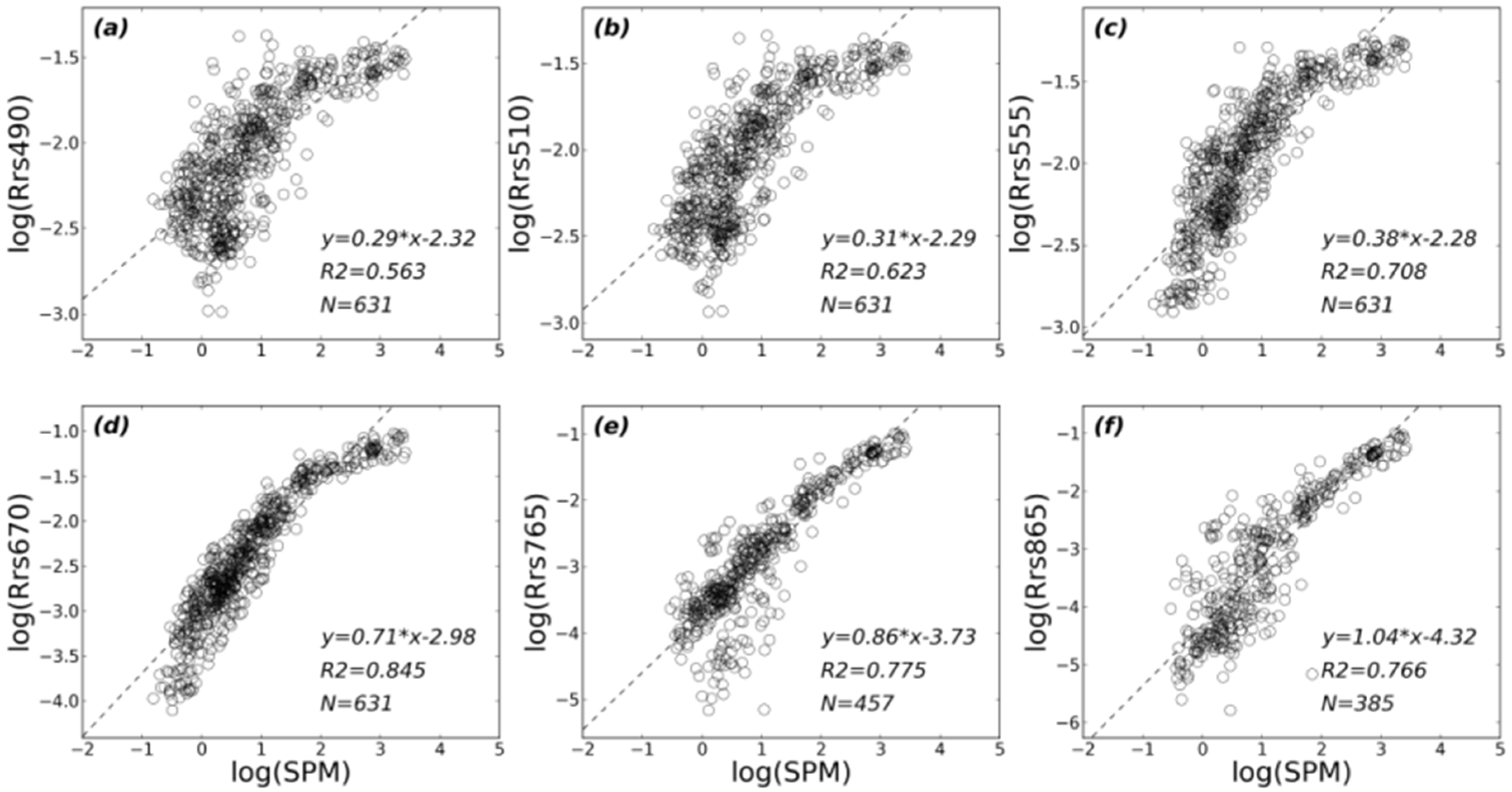
3.1. General Trends between R_rs and SPM

The correlation between R_rs and SPM was analyzed in logarithmic scale for the wavelengths available on current ocean color sensors prior to the development and validation of the SPM algorithms (Figure 4). As already mentioned in previous studies [12,26], the correlation coefficient between R_rs and SPM increases from the blue to the red spectral domain. For instance, the determination coefficient, R², increases from 0.563 at 490 nm (Figure 4a) to 0.775 at 765 nm (Figure 4e). In the same way, the scatter observed around the R_rs vs.SPM relationship continuously decreases from the blue to the red part of the spectrum. These two observations can be related to the increase with the wavelength of the relative contribution of pure water absorption to the total absorption coefficient, as well as to the increasing influence of the particulate backscattering coefficient, b_bp, on the R_rs variability. While the R_rs values measured in the visible part of the spectrum tend to saturate from SPM values of about 50 g·m⁻³ (Figure 4c,d), the linearity between log(R_rs) and log(SPM) is recovered in the near-infrared part of the spectrum (Figure 4e,f). This is consistent with previous studies [4,19,20,51] and can be explained by the fact that pure water absorption, a_w, increases by almost a factor of 10 from the red to the NIR part of the spectrum. For highly turbid waters, as R_rs can be approximated by the b_b/(a+b_b) ratio, R_rs is only driven by b_bp in the NIR, whereas this ratio (and thus R_rs) does not sharply increase in the red, as b_b and a are globally at the same order of magnitude. Note however that, while the slope in the log(R_rs(670)) vs. log(SPM) relationship changes from turbid to highly turbid waters (Figure 4d), R_rs(670) is still sensitive to SPM variability in such very turbid environments. This feature is important, considering that the accuracy in the R_rs estimate in the NIR has still not been fully evaluated, creating therefore potential doubt in the use of such NIR channel for evaluating SPM concentration. In the same way, the correlation between SPM and four different R_rs band ratios (all with respect to the green band, i.e., 555 nm for SeaWiFS) has also been examined (Figure 5). Among the four band ratios investigated here, the red-to-green band ratio, R_rs(670)/R_rs(555), is the one which exhibits the best correlation with SPM when the full SPM range is considered. Similar to the case of a single R_rs band, near-infrared-to-green band ratios such as R_rs(765)/R_rs(555) and R_rs(865)/R_rs(555)are only well related with SPM for highly and extremely turbid waters.

3.2. Performance of Historical Algorithms

The equations of the four previously published algorithms selected for the present study are provided below for the SeaWiFS sensor.

(1) “Siswanto11” model (Siswanto et al. [24])

log₁₀(SPM) = 0.649 + 25.623 · X₁ + 0.646 · X₂

(9)

where X₁ = R_rs(555) + R_rs(670), X₂ = R_rs(490)/R_rs(555).

(2) “Nechad10” model (Nechad et al. [26])

SPM = 384.11·ρ_w(670)/(1 −ρ_w(670)/0.1747) + 1.44

(10)

where ρ_w(670) = π∙R_rs(670).

(3) “Doxaran03” model (Doxaran et al. [20])

SPM = 26.083 × exp(0.336X)

(11)

where X = R_rs(865)/R_rs(555). Note: this model was tuned for SPM greater than 10 g·m⁻³.

(4) “Gohin05” model (Gohin et al. [29])

SPM = nLvSPM(nL_w(555), nL_w(670)) + 234 Chl^0.57

(12)

The look-up tables required for the Chl calculations and the coefficients required for the SPM calculations were provided by ACRI-HE with the agreement of IFREMER.

The performance of these algorithms (Equations (9)–(12)), belonging to three different inverse approaches, are tested over the DS-T data set (Figure 6). The Siswanto11 model (Figure 6a), originally developed on SPM values ranging between 0.04 and 340 g·m⁻³, provides the best retrieval accuracy with an RMSE_log of 0.33 over the whole SPM range considered in this study. This model tends, however, to underestimate SPM in relatively clear waters and, overestimate SPM in extremely turbid waters. The semi-analytical approach by Nechad et al. (2010) [26], Nechad10, also shows fairly good performance in SPM retrieval (RMSE_log= 0.39), although with certain inherent limitations at low high SPM concentrations (Figure 6b), explaining the high Bias value of about 180%. This algorithm, developed from SPM values greater than 1.2 g·m⁻³, leads to over-estimation of SPM at low concentration, due to the adoption of a constant offset (i.e., 1.44 g·m⁻³ for B^ρ) which is reached for low R_rs(670) values. As soon as ρ_w(670)(= π∙R_rs(670)) is greater than 0.1747 (a situation frequently encountered in highly to extremely turbid waters), negative SPM values can also be generated (37 cases encountered in DS-T, not shown in Figure 6b). Such highly turbid waters were not considered in the calibration data set used by Nechad et al. (2010) [26] as their maximum SPM value reached 110.3 g·m⁻³ only. As expected, the Doxaran03 model appears to be fairly valuable for highly and extremely turbid waters (Figure 6c), but fails to perform well for low to medium SPM, as this model was originally developed for SPM values ranging between 10 and 2000 g·m⁻³. It should also be noted that the number of valid R_rs(λ)-SPM data points decreases significantly in DS-T when R_rs in the near-infrared range is used (e.g., 865 nm for SeaWiFS). The Gohin05 model (Gohin et al., 2005 [29]) provides relatively good retrieval of SPM for low to medium SPM concentrations, but is not able to accurately estimate SPM for concentration higher than about 50 g·m⁻³. The RMSE_log and bias values decrease from 0.376% and 127.3%, respectively, when the whole data set is considered, to 0.363 and 118%, when in situ SPM concentrations lower than 10 g·m⁻³ only are considered. Better SPM retrievals could certainly be achieved through, for instance, the improvement of the standard specific IOPs values used in the model, as already mentioned in Gohin (2011) [48]. Recently, the model has been improved thanks to a collaboration between IFREMER (F. Gohin) and the University of Bangor in Wales (D. Bowers). Unfortunately, this version is not available yet.

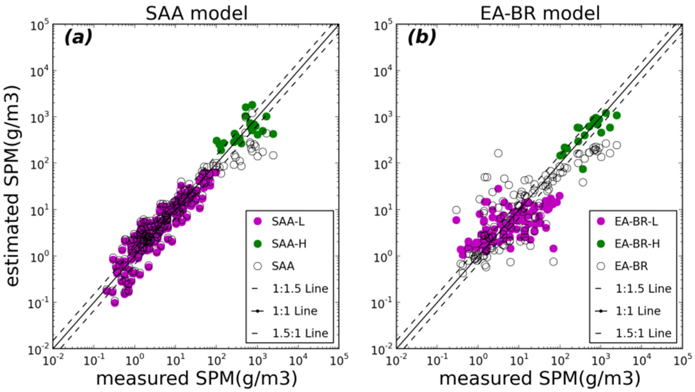
3.3. Performance of Tuned Algorithms

The Siswanto-, Nechad-, and Doxaran-like models, as described in Equations (1)–(3), have been fitted to our development dataset (DS-D) in order to assess if these formulations can be used to retrieve SPM spanning about four orders of magnitude. The new coefficients are provided in Table 3. Based on the relationship between R_rs band ratio and SPM, as shown in Figure 5, EA-BR model is re-designed to be in the form of SPM~a₀∙X^a1, where X is the R_rs band ratio. To avoid the cut-off situation encountered at low SPM range (Figure 6b), the offset parameter in Nechad-like model has been removed for this fitting exercise (i.e., B^ρ = 0 in Equation (3)). Logically, the newly tuned models provide much better SPM retrieval when compared to their original version, as emphasized by the statistics computed from the independent DS-V data set (Figure 7 and

Table 4. Statistics of original (Equations (9)–(12)) and re-tuned models (Table 3 computed based on the validation sub-dataset (DS-V).

Model Reference	BIAS (%)	MRAD (%)	Ratio	RMSE_log	N
Siswanto11	41.5	75.5	1.42	0.33	196
Nechad10	98.7	130.1	1.99	0.37	186
Doxaran03	208.8	208.8	3.09	0.91	132
Gohin05	127.3	134.2	2.27	0.38	196
EA-MB	20.6	62.5	1.21	0.32	196
EA-MB-L 1	13.6(17.5)	55.0(55.9)	1.14(1.18)	0.29(0.29)	174
EA-MB-H 1	39.7(45.0)	77.9(114.9)	1.40(1.45)	0.35(0.51)	22
SAA	22.3	57.6	1.22	0.31	196
SAA-L 1	16.4(31.2)	50.0(57.1)	1.16(1.31)	0.26(0.26)	174
SAA-H 1	−15.4(−63.9)	59.7(71.6)	0.85(0.36)	0.34(0.65)	22
EA-BR	142.4	202.9	2.42	0.55	132
EA-BR-L 1	49.8(162.5)	113,1(213.1)	1.50(2.63)	0.51(0.55)	110
EA-BR-H 1	10.5(−65.8)	35.5(65.8)	1.11(0.34)	0.22(0.58)	22

¹ numbers shown in parentheses in EA-MB-L, EA-MB-H, SAA-L, SAA-H, EA-BR-L and EA-BR-H rows represent corresponding statistics when EA-MB, SAA and/or EA-BR model are applied instead.

). For instance, the bias values decrease by about a factor of two between the original and fitted EA-MB and EA-BR models, and by a factor of four for the SAA algorithm. This improvement is mainly due to the fact that original models were not developed for such a wide range in SPM concentration. The relatively higher scatter observed around the 1:1 line for the EA-BR model is related to the fact that this NIR based model was originally designed for medium to extremely turbid waters [20] for which signal to noise ratio is sufficiently high to draw a significant relationship between SPM and R_rs at the considered wavelengths. The reversal feature explains the very high scatter observed for low to moderate SPM values thus confirming the inability of such NIR formulation to be used over the whole range of turbidity encountered in contrasted coastal waters (as already emphasized in Figure 4f and Figure 5d).

Both SAA (Figure 7b) and EA-MB (Figure 7c) models perform relatively well for clear to medium turbid waters, but misestimate SPM in highly to extremely turbid environments. For instance, the RMSE_log value increases from 0.32 to 0.51 when the EA-MB model is applied for waters characterized by SPM concentration higher than 100 g·m⁻³. In the same way, the RMSE_log value for the SAA model increases from 0.31 to 0.65 for SPM concentration higher than 100 g·m⁻³. This feature clearly indicates that the SPM range should be explicitly taken into account within the inverse procedure development.

3.4. New Formulations

3.4.1. Performance of SPM-Range Dependent Algorithms

The previous results underline the inability of the three considered algorithms, even re-tuned on the DS-D data set, to properly deliver SPM over the whole SPM range considered. This can be more likely associated with the fact that the considered formulations and thus the hypotheses shaping these models are not able to fully capture the dynamics in the R_rs-SPM relationships over about four orders of magnitude in SPM concentration. The latter results thus tend to indicate that turbidity conditions should be explicitly included in the inversion procedure if the aim is to deliver SPM concentration over extremely contrasting marine environments. In order to illustrate this feature, a first approach can consist in re-defining the three selected algorithms according to two different SPM ranges arbitrarily fixed to SPM higher and lower than 100 g·m⁻³. For each of the three models (SAA, EA-MB, and EA-BR), two distinct sub-models have been developed considering low (L) and high (H) SPM conditions. Each sub-model is derived by retuning the coefficients appearing in Equations (1)–(3), in the two SPM ranges based on the DS-D dataset. Note the modification of EA-BR model (see Section 3.3). Even though 100 g·m⁻³ seems arbitrary, it should represent a credible threshold from a qualitative perspective (see Figure 7). A proper selection of an optical segment index will be specifically assessed in the following section.

The SPM-range dependent algorithms allow SPM to be retrieved with a much better accuracy for the former two considered approaches (i.e., SAA and EA-BR models, Figure 8 and Table 4). For instance, the RMSE_log value decreases from 0.65 to 0.34 for SAA and from 0.58 to 0.22 for EA-BR, for SPM concentrations higher than 100 g·m⁻³. The same results are observed, to a lesser extent, for the lower SPM range (Table 4). For instance, the RMSE_log value decreases from 0.36 to 0.26 when the SAA and SAA-L models are used, respectively, in this lower SPM range (SPM < 100 g·m⁻³).Note that the EA-MB model is not considered in Figure 8 because the SPM-range dependent approach was not able to give better results than the former EA-MB model.

3.4.2. Generic Semi-Analytical Model

Because of its physical foundation, as well as its slightly better performance compared to the two empirical approaches considered here, the generic algorithm is developed based on the SAA formulation only. As previously emphasized, SPM concentration can be retrieved with a substantially improved accuracy when clear to medium turbid waters and highly to extremely turbid waters are considered separately. The applicability of such an inversion algorithm is, however, conditioned by the possibility to define a switching point between these latter two turbidity conditions based on an optical criterion. Among the several optical switching indexes possible (e.g., single band or band ratio based threshold), the remote-sensing reflectance, R_rs, in the red domain (i.e., 670 nm for SeaWiFS) was found to be the most valuable proxy for defining on a pixel basis low-medium or high turbidity environment, and thus for choosing the proper SPM inversion algorithm. However, considering that remote-sensing reflectance at red wavelength may saturate for the extremely high SPM range, while one algorithm has been developed for the low-medium SPM range (named SAA-L), two different algorithms have to then be tested for the higher SPM range. The first one (named SAA-HR) used R_rs in the red, while the second one (named SAA-HNIR), which should be more sensitive to very high SPM concentrations, used R_rs in the near-infrared waveband (i.e., 765 nm for SeaWiFS).

In order to determine an appropriate threshold based on a radiometric index (e.g., single band or band ratio), two situations are considered separately. One heuristic way consists in considering an increasing threshold value, then to re-formulate model coefficients for each critical value, and compare the evolution in the performance of the SPM inversion for the two sub-validation datasets as defined by the chosen threshold. This first approach is defined as the “lower critical value”. The same procedure can be applied to the other direction considering an index that is confined to be not much greater than a gradually decreasing critical value (“upper critical value”). The determination of both optimal values is assessed from the validation statistics and requires a sufficient number of records to ensure the test’s representativeness. Both single band and band ratios can be considered as a possible index. However, single band remote-sensing reflectance can be assumed to represent a more suitable index since it correlates with SPM in a more straightforward way than band ratio does. By iterating lower and upper critical values of R_rs(670), for the case of the SeaWiFS sensor, 0.03 and 0.04 sr⁻¹ have been determined from the current data set as optimal lower and upper critical values, respectively. The coefficients for these three algorithms using the DS-D data set are provided in

Table 5. Coefficients of the SPM-dependent models developed on DS-D for various Ocean Color sensors.

Model Index	Sensor Name	WavebandsInvolved (nm) 1	Switching Threshold	Retuned Coefficients 2	N
SAA-L	SeaWiFS	670	Rrs(670) ≤ 0.03	391.161, 0.5	366
	MODIS-A	667	Rrs(667) ≤ 0.03	404.400, 0.5	366
	MODIS-T	667	Rrs(667) ≤ 0.03	404.400, 0.5	366
	MERIS/OLCI/MSI	665	Rrs(665) ≤ 0.03	396.005, 0.5	365
	VIIRS	671	Rrs(671) ≤ 0.03	389.471, 0.5	366
	OLI	655	Rrs(655) ≤ 0.03	346.353, 0.5	362
SAA-HR	SeaWiFS	670	Rrs(670) ≥ 0.04	1336.584, 0.3864	49
	MODIS-A	667	Rrs(667 ≥ 0.04	1214.669, 0.3394	46
	MODIS-T	667	Rrs(667) ≥ 0.04	1214.669, 0.3394	46
	MERIS/OLCI/MSI	665	Rrs(665) ≥ 0.04	1208.481, 0.3375	46
	VIIRS	671	Rrs(671) ≥ 0.04	1234.599, 0.3439	47
	OLI 3	655	Rrs(655) ≥ 0.045	1221.390, 0.3329	38
SAA-NIR	SeaWiFS	765	Rrs(670) ≥ 0.04	2245.985, 0.4168	49
	MODIS-A	748	Rrs(667 ≥ 0.04	2201.029, 0.3975	46
	MODIS-T	748	Rrs(667) ≥ 0.04	2201.029, 0.3975	46
	MERIS/OLCI/MSI 4	753	Rrs(665) ≥ 0.04	2220.066, 0.4029	46
	VIIRS	745	Rrs(671) ≥ 0.04	2198.675, 0.3951	47
	OLI 4	-	-	-	-

¹ Selected wavebands (i.e., λ₀) in Equation (2). ² Retuned coefficients for A^ρ and C^ρ in Equation (2), respectively, while B^ρ = 0; ³ For OLI (center wavelength = 655 nm), 0.045 sr⁻¹ works better as upper switching point than 0.04 sr⁻¹; ⁴ MSI and OLI do not have wavebands in the near-infrared domain (e.g., 765 nm for SeaWiFS).

.

Table 6. Validation of SPM-dependent models on DS-V.

Model Name	Sensor Name	Switching Threshold	Bias (%)	MRAD (%)	Ratio	RMSE_log	N
SAA-L	SeaWiFS	Rrs(670) ≤ 0.03	17.8	51.4	1.18	0.263	166
	MODIS-A	Rrs(667) ≤ 0.03	18.4	51.9	1.18	0.263	166
	MODIS-T	Rrs(667) ≤ 0.03	18.4	51.9	1.18	0.263	166
	MERIS/OLCI/MSI	Rrs(665) ≤ 0.03	18.8	52.5	1.19	0.264	165
	VIIRS	Rrs(671) ≤ 0.03	17.5	51.2	1.18	0.263	166
	OLI	Rrs(655) ≤ 0.03	15.5	50.6	1.16	0.261	166
SAA-HR	SeaWiFS	Rrs(670) ≥ 0.04	−0.4	52.1	1.00	0.329	18
	MODIS-A	Rrs(667 ≥ 0.04	9.7	59.0	1.10	0.340	18
	MODIS-T	Rrs(667) ≥ 0.04	9.7	59.0	1.10	0.340	18
	MERIS/OLCI/MSI	Rrs(665) ≥ 0.04	10.0	59.4	1.10	0.342	18
	VIIRS	Rrs(671) ≥ 0.04	9.7	58.4	1.10	0.337	18
	OLI 1	Rrs(655) ≥ 0.045	2.5	56.3	1.03	0.347	16
SAA-HNIR	SeaWiFS	Rrs (670) ≥ 0.04	06.5	40.7	0.94	0.277	18
	MODIS-A	Rrs(667 ≥ 0.04	−5.6	41.7	0.94	0.282	18
	MODIS-T	Rrs(667) ≥ 0.04	−5.6	41.7	0.94	0.282	18
	MERIS/OLCI	Rrs(665) ≥ 0.04	−5.9	41.4	0.94	0.281	18
	VIIRS	Rrs(671) ≥ 0.04	−5.2	42.0	0.95	0.282	18
	OLI	-	-	-	-	-	-

¹ For OLI (center wavelength = 655 nm), 0.045 sr⁻¹ works more effectively as an upper switching point than 0.04 sr⁻¹.

gives statistics when these SPM-dependent models are validated using DS-V.

The consideration of two distinct algorithms based on the relative turbidity of the water masses for remote sensing application might induce an artificial spatial pattern in the SPM distribution. To prevent such possible irregularity, a smoothing procedure has thus to be applied especially for regions intermediary between medium and high turbid situations. The smoothing method adopted consists in defining a weighting function of the low-medium and high SPM algorithms. In practice, two weights (W_L and W_H for low and high SPM conditions, respectively) have been defined as follows:

$${\mathrm{W}}_{\mathrm{L}}=\{\begin{array}{c}1,\mathrm{if}{R}_{\text{rs}}\left({\mathsf{\lambda }}_0\right)\le 0.03{\mathrm{sr}}^{-1}\\ 0,\mathrm{if}{R}_{\text{rs}}\left({\mathsf{\lambda }}_0\right)\ge 0.04{\mathrm{sr}}^{-1}\\ {\text{log}}_{10}\left(0.04\right)-{\text{log}}_{10}\left[R_{\text{rs}}\left({\mathsf{\lambda }}_0\right)\right],\mathrm{otherwise}\end{array}$$

(13)

$${\mathrm{W}}_{\mathrm{H}}=\{\begin{array}{c}0,\mathrm{if}{R}_{\text{rs}}\left({\mathsf{\lambda }}_0\right)\le 0.03{\mathrm{sr}}^{-1}\\ 1,\mathrm{if}{R}_{\text{rs}}\left({\mathsf{\lambda }}_0\right)\ge 0.04{\mathrm{sr}}^{-1}\\ {\text{log}}_{10}\left[R_{\text{rs}}\left({\mathsf{\lambda }}_0\right)\right]-{\text{log}}_{10}\left(0.03\right),\mathrm{otherwise}\end{array}$$

(14)

where λ₀ is 670 nm, 667 nm, 667 nm, 665 nm, 671 nm and 655 nm for SeaWiFS, MODIS-A, MODIS-T, MERIS/MSI/OLCI, VIIRS and OLI, respectively. The weighted SPM is then computed as:

$$SPM=\frac{{\mathrm{W}}_{\mathrm{L}}·SP{M}_{\mathrm{L}}+{\mathrm{W}}_{\mathrm{H}}·SP{M}_{\mathrm{H}}}{{\mathrm{W}}_{\mathrm{L}}+{\mathrm{W}}_{\mathrm{H}}}$$

(15)

Where SPM_L and SPM_H are estimated by models calibrated for low turbidity (i.e., SAA-L) and high turbidity(i.e., SAA-HR or SAA-HNIR) environments, respectively.

These two sets of algorithms, that is SAA-L combined with SAA-HR, and SAA-L combined with SAA-HNIR, are applied to the in situ data set DS-V to evaluate their respective performance (

Table 7. Performance of combined SPM-dependent models for various ocean color sensors on DS-V.

Model Name	Sensor Name	RPD (%)	APD (%)	Ratio	RMSE_log	N
Switch_1	SeaWiFS	19.6	54.5	1.20	0.274	196
	MODIS-A	21.1	55.5	1.21	0.275	196
SAA-L+	MODIS-T	21.1	55.5	1.21	0.275	196
	MERIS/OLCI/MSI	21.5	56.0	1.22	0.275	196
SAA-HR	VIIRS	20.1	54.7	1.20	0.274	196
	OLI	20.3	54.2	1.20	0.270	196
Switch_2	SeaWiFS	15.5	50.1	1.16	0.261	196
	MODIS-A	16.3	50.7	1.16	0.262	196
SAA-L+	MODIS-T	16.3	50.7	1.16	0.262	196
	MERIS/OLCI/MSI 1	16.5	51.0	1.17	0.262	196
SAA-HNIR	VIIRS	15.4	50.0	1.15	0.261	196
	OLI 1	-	-	-	-	-

¹ MSI and OLI do not have wavebands in the near-infrared spectral domain comparable to that of other Ocean Color sensors (e.g., 765 nm for SeaWiFS).

). Compared to the performances reached by the SAA algorithm developed over the whole SPM range, the application of the SPM-range dependent algorithms provides a much better SPM retrieval. For instance, the RMSE_log value calculated over the whole SPM range is 0.31 for SAA, 0.27 for combination of (SAA-L, SAA-HR), and 0.26 for that of (SAA-L, SAA-HNIR), respectively (Table 7). Compared to SAA (Table 4), the Bias value decreases by a factor of 1.27 and 1.44 for (SAA-L, SAA-HR), and (SAA-L, SAA-HNIR), respectively. At high turbid waters (e.g., R_rs(670) ≥ 0.04 sr⁻¹), the SAA-HNIR (RMSE_log = 0.28; MRAD = 40.7%) presents slightly better SPM retrieval than SAA-HR (RMSE_log = 0.33; MRAD = 52.7%). This difference observed between SAA-HR and SAA-HNIR is simply explained by the tighter linear behavior between R_rs and SPM in the near-infrared than in the red part of the spectrum (Figure 4). The latter general statistics vary only slightly from one sensor to another (i.e., SeaWiFS, MODIS, MERIS VIIRS, OLCI, OLI, MSI) demonstrating the great potential applicability of using such combined approaches (Table 7).

Further, the application of such a smoothing procedure (Equations (13)–(15)) on MERIS data confirms that the switching and smoothing method proposed here allows the prevention of any artificial discontinuity in the SPM coastal to offshore dispersion gradient (see Figure 9). The SPM retrieval follows the same spatial course as the one described by R_rs(665), with no obvious discontinuity observed at the switching domain, that is for R_rs(665) values between 0.03 and 0.04 sr⁻¹. Besides, the estimation of concentration as high as 1300 g·m⁻³ (around the latitude 48.8°S in Figure 8b) clearly stresses that the use of the remote sensing reflectance in the red, combined with this switching method, is totally adapted to very turbid waters.

4. Sensitivity Analysis

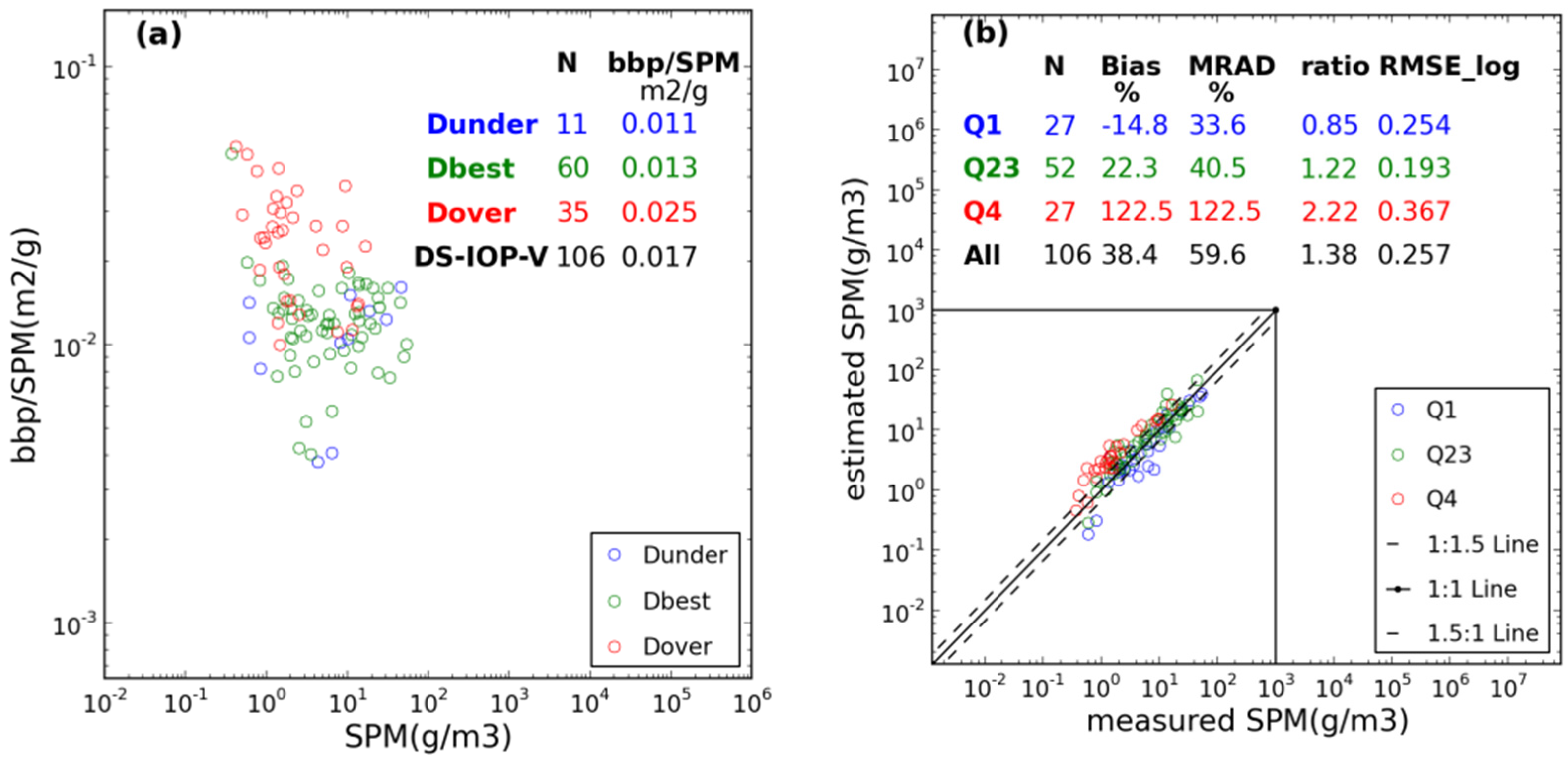
4.1. Sensitivity of the SPM Retrieval Accuracy to the b_bp/SPM Variability

This section aims at verifying whether the accuracy of the SPM retrieval is partly linked to the SPM mass-specific backscattering coefficient ($b_{\text{bp}}^{*}$) variability. This exercise is performed for the SAA algorithm only. From the SPM retrieved values using this latter algorithm (Figure 10), three subsets of data were generated based on the ratio value of estimated to measured SPM as computed from DS-IOP-V. The first group (D_over) gathers data with a ratio value greater than 1.5 (significantly over-estimated SPM), while the second group (D_under) concerns data with a ratio lower than 1/1.5 (significantly under-estimated SPM). The remaining data points, which represent the best estimated SPM values, lie in the third group (D_best). The mean $b_{\text{bp}}^{*}\left(488\right)$ calculated for the data points gathered into D_over (0.025 ± 0.011 m²·g⁻¹) is about two times higher than the one calculated over D_under (0.011±0.004 m²·g⁻¹) (Figure 10a). Interestingly, the remaining data points for which the estimation of SPM from the SAA algorithm is relatively good, present intermediate $b_{\text{bp}}^{*}\left(488\right)$ value (0.013 ± 0.006 m²·g⁻¹). This result strongly emphasizes that the accuracy in the SPM retrieval is tightly linked to the bulk particulate matter chemical composition and size. Higher $b_{\text{bp}}^{*}\left(488\right)$ values are, for instance, generally observed for waters where the particulate fraction is dominated by the presence of mineral particles [37]. These results regarding the impact of the specific backscattering coefficient on the SPM retrieval are in line with the study of Binding et al. (2005) [51] performed on moderately turbid waters.

The actual effect of the variability in $b_{\text{bp}}^{*}$ on SPM retrieval has been examined quantitatively. For that purpose, DS-IOP-V is re-organized into three sub-groups based on quartiles in terms of $b_{\text{bp}}^{*}$ following the Loisel et al.’s (2010) approach [45]. The first quartile cuts off the lowest 25% of the $b_{\text{bp}}^{*}$ data. The corresponding sub data set is named DS-IOP-VQ1. The third quartile cuts off the highest 25% into a sub-dataset named DS-IOP-VQ4. The remaining goes into DS-IOP-VQ23. The SPM-retrieval accuracy through the use of SAA significantly differs between DS-IOP-VQ1 and DS-IOP-VQ4 (Figure 10b). For instance, a negative bias of −21.1% is observed for the data point of DS-IOP-VQ1, while a positive bias of 74.8% is observed for DS-IOP-VQ4.

In the SAA model (see Section 2.2), C^ρ is related to $b_{\text{bp}}^{*}$ through ${\mathrm{C}}^{\mathsf{\rho }}=\mathsf{\gamma }·b_{\text{bp}}^{*}/\left(a_{\mathrm{p}}^{*}+b_{\text{bp}}^{*}\right)$, with $a_{\mathrm{p}}^{*}$ and γ held constant and taken from Nechad et al. (2010) [26], while A^ρ (see Equation (3)) is determined through a non-linear least square fit. A general model (called “M0”) was obtained considering the whole DS-IOP-D data set. Similarly, for each quartile-based sub-group of DS-IOP-D (i.e., DS-IOP-DQ1, DS-IOP-DQ23 and DS-IOP-DQ4, the same division is applied to DS-IOP-V), new sets of C^ρ and A^ρ were calculated leading to three associated models (“M1”, “M23”, and “M4”). The performance of these three models was evaluated over the DS-IOP-V data set (Figure 11). A substantial improvement is observed over the DS-IOP-VQ1 and DS-IOP-VQ4 data sets when the model parameters are adjusted regarding to their mean $b_{bp}^{*}$ values. For instance, the RMSE_log value decreases from 0.318 (with “M0” model) to 0.264 (with “M1” model) for DS-IOP-VQ1. In the same way, the RMSE_log value decreases from 0.277 (with” M0” model) to 0.172 (with “M4” model) for DS-IOP-VQ4. Besides, the SPM retrieval accuracy remains equivalent between “M0” and “M23” model. The same result has been observed for the other algorithms presented here (not shown). These results strongly emphasize that implicit knowledge on the $b_{bp}^{*}$ values, combined with appropriated SAA algorithms, would significantly improve the SPM assessment from the marine reflectance (at least for the SPM range tested here).

4.2. Effect of Rrs Uncertainties on the SPM Retrieval

The impact R_rs retrieval errors, mainly caused by uncertainties in the atmospheric correction procedure, on the SPM retrieval accuracy was examined for the EA-BR, SAA and EA-MB models. For that purpose, relative error budget for the R_rs signal in the blue, green, and red domains was assumed to be normally distributed with mean (and standard deviation) values of −0.2% (0.05%), −3% (0.6%), and −25% (5%), respectively. The latter mean values were fixed according to the results of the match-up exercise performed for the MODIS-aqua sensor using the NASA standard NIR-atmospheric correction scheme [52]. Statistically, R_rs uncertainties causes SPM to be under-estimated for all cases, with RMSE_log increases from 0.554, 0.307, and 0.320 to 0.657, 0.363, and 0.374 for EA-BR, SAA and EA-MB models, respectively.

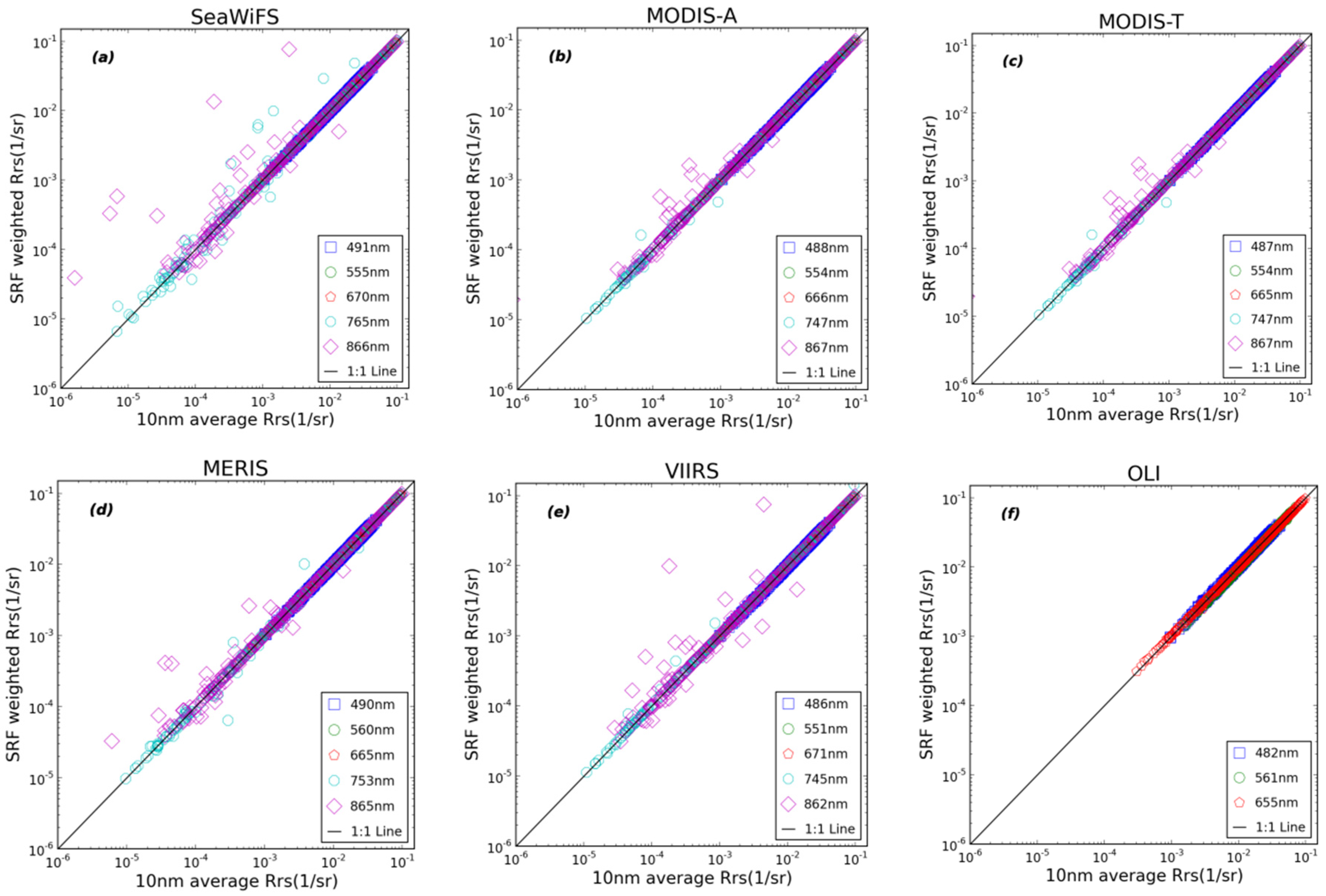
4.3. Impact of the Spectral Response Function of Each Ocean Color Sensors

The models developed in this study were developed from coinciding in situ R_rs and SPM measurements. Specifically, R_rs were calculated over a 10 nm-bandwidth whenever possible i.e., for hyper-spectral measurements. However, in order to check for the ability of the proposed models to be applied to the different ocean color sensors available, R_rs data should be weighted according to the corresponding Spectral Response Functions, SRF, for each ocean color sensor [53]. This step, which is recommended in the case of high spatial resolution sensors with large spectral bandwidths such as SPOT [54] or Landsat ETM+ [11], is here tested with narrow bands of ocean color sensors. Comparison between these two sets of R_rs (i.e., averaged over 10 nm, or using the appropriated SRF) is performed for the selected bands of SeaWiFS, MODIS-Aqua, MODIS-Terra, MERIS, VIIRS and OLI sensors (Figure 12), respectively. Except for several points in the near-infrared spectral region which significantly deviate from the 1:1 line, R_rs data calculated by the two methods are in perfect agreement (Figure 12). This indicates that previously re-tuned models can be applied without any change to ocean color remote sensing data provided by these sensors. In the near-infrared domain, SRF usually covers a large band width (i.e., 40 nm or more), making it more vulnerable to abnormal values. Therefore, one should be very careful about the quality control for this part of the spectrum.

5. Concluding Remarks

From an extensive in situ data set covering about four orders of magnitude in SPM, some historical SPM inversion algorithms based on different approaches have been evaluated. While these algorithms usually performed relatively well over the SPM range used for their development, they typically fail outside of these defined ranges. Because of the sensitivity of the different algorithms to the level of turbidity, generic algorithms based on a switching criteria, according to the R_rs value in the red (i.e., 670 nm for SeaWiFS), have been proposed in the present study. Due to its generally better performance and to its semi-analytical formulation, the SAA model has been selected as the most appropriate algorithm for the SPM assessment. Besides, compared to other approaches, SAA has the advantage to be easily adapted to the optical environment encountered. For instance, we have shown a great improvement in the SPM retrieval accuracy when parameters of the algorithm were adapted to the b_bp/SPM values encountered in the observed water mass. Environments with high or low b_bp/SPM values (mineral vs. phytoplankton dominated waters) could be distinguished from classification approaches [40,55,56], or through the use of polarization measurements [57], allowing the improvement of the SPM retrieval if such information is made available.

Taking SeaWiFS as an example, while R_rs(670) is used as the input parameter in SAA for low to medium turbid waters, R_rs(670) or R_rs(765) can be chosen for very turbid waters. The retrieval accuracy of SPM in highly turbid waters is only slightly improved when R_rs(765) is chosen instead of R_rs(670). Indeed, even if R_rs(765) presents more dynamics than R_rs(670) in very turbid waters (as explained in Section 3.1), a significant R_rs(670) vs. SPM relationship can still be established. The use of this relationship allows SPM to be estimated with a satisfactory accuracy. The preference in the SAA-HR compared to the SAA-HNIR option is thus motivated by the following reasons. First, the retrieval accuracy between the two options is very similar. Second, the signal to noise ratio in the NIR channel is generally lower than in the red [58]. This is true for SeaWiFS and MERIS but not for MODIS which presents about the same SNR in these two spectral domains. Third, while the channel centered at around 670 nm is available for all the sensors, this is not the case for 765 nm (i.e., Landsat8/OLI). At last, the retrieval accuracy of R_rs(765), obtained after the atmospheric correction procedure, has still not been estimated, as thus compared with 670 nm. While in situ measurements have shown that SAA-HR and SAA-HNIR provide about the same SPM retrieval accuracy over very turbid waters, a first test on real satellite data over different turbid areas (not shown here)has revealed that estimated SPM values are much lower with SAA-HNIR than with SAA-HR. This pattern clearly emphasizes the necessity to better evaluate the R_rs in the near infrared spectral domain.

References

1. Loisel, H.; Mangin, A.; Vantrepotte, V.; Dessailly, D.; Dinh, D.; Garnesson, P.; Ouillon, S.; Lefebvre, J.-P.; Meriaux, X.; Phan, T. Variability of suspended particulate matter concentration in coastal waters under the Mekong’s influence from ocean color (MERIS) remote sensing over the last decade. Remote Sens. Environ. 2014, 150, 218–230. [Google Scholar]
2. Vanhellemont, Q.; Ruddick, K. Turbid wakes associated with offshore wind turbines observed with Landsat 8. Remote Sens. Environ. 2014, 145, 105–115. [Google Scholar] [CrossRef]
3. Fettweis, M.; Nechad, B.; Den, E.D. An estimate of the suspended particulate matter (SPM) transport in the southern North Sea using SeaWiFS images, in situ measurements and numerical model results. Cont. Shelf Res. 2007, 27, 1568–1583. [Google Scholar] [CrossRef]
4. Doxaran, D.; Froidefond, J.M.; Lavender, S. Spectral signature of highly turbid waters: Application with SPOT data to quantify suspended particulate matter concentrations. Remote Sens. Environ. 2002, 81, 149–161. [Google Scholar] [CrossRef]
5. Toth, B.; Bodis, E. Estimation of suspended loads in the Danube River at Göd (1668 river km), Hungary. J. Hydrol. 2015, 523, 139–146. [Google Scholar] [CrossRef] [Green Version]
6. Pedersen, T.; Gallegos, C.; Nielsen, S. Influence of near-bottom re-suspended sediment on benthic light availability. Estuar. Coast. Shelf Sci. 2012, 106, 93–101. [Google Scholar]
7. Martin, J.M.; Windom, H.L. Present and future roles of ocean margins in regulating marine biogeochemical cycles of trace elements. In Ocean Margin Processes in Global Change; Mantoura, R.F.C., Martin, J.M., Wollast, R., Eds.; John Wiley & Sons: Hoboken, NJ, USA, 1991; pp. 45–67. [Google Scholar]
8. Ko, F.; Baker, J. Seasonal and annual loads of hydrophobic organic contaminants from the Susquehanna River basin to the Chesapeake Bay. Mar. Pollut. Bull. 2004, 48, 840–851. [Google Scholar] [CrossRef] [PubMed]
9. Mayer, L.; Keil, R.; Macko, S. Importance of suspended participates in riverine delivery of bioavailable nitrogen to coastal zones. Glob. Biogeochem. Cycles 1998, 12, 573–579. [Google Scholar] [CrossRef]
10. Woźniak, S. Simple statistical formulas for estimating biogeochemical properties of suspended particulate matter in the southern Baltic Sea potentially useful for optical remote sensing applications. Oceanologia 2014, 56, 7–39. [Google Scholar] [CrossRef]
11. Ouillon, S.; Douillet, P.; Andrefouet, S. Coupling satellite data with in situ measurements and numerical modeling to study fine suspended-sediment transport: A study for the lagoon of New Caledonia. Coral Reefs 2004, 23, 109–122. [Google Scholar]
12. Ouillon, S.; Douillet, P.; Petrenko, A.; Neveux, J.; Dupouy, C.; Froidefond, J.M.; Andréfouët, S.; Muñoz-Caravaca, A. Optical algorithms at satellite wavelengths for total suspended matter in tropical coastal waters. Sensors 2008, 8, 4165–4185. [Google Scholar] [CrossRef]
13. Moore, G.; Aiken, J.; Lavender, S. The atmospheric correction of water colour and the quantitative retrieval of suspended particulate matter in Case II waters: Application to MERIS. Int. J. Remote Sens. 2010, 20, 1713–1733. [Google Scholar] [CrossRef]
14. Miller, R.; Mckee, B. Using MODIS Terra 250 m imagery to map concentrations of total suspended matter in coastal waters. Remote Sens. Environ. 2004, 93, 259–266. [Google Scholar] [CrossRef]
15. Hu, C.; Chen, Z.; Clayton, T. Assessment of estuarine water-quality indicators using MODIS medium-resolution bands: Initial results from Tampa Bay, FL, USA. Remote Sens. Environ. 2004, 93, 423–441. [Google Scholar] [CrossRef]
16. Zhang, M.; Tang, J.; Dong, Q. Retrieval of total suspended matter concentration in the Yellow and East China Seas from MODIS imagery. Remote Sens. Environ. 2010, 114, 392–403. [Google Scholar] [CrossRef]
17. Min, J.; Ryu, J.; Lee, S. Monitoring of suspended sediment variation using Landsat and MODIS in the Saemangeum coastal area of Korea. Mar. Pollut. Bull. 2012, 64, 382–390. [Google Scholar] [CrossRef] [PubMed]
18. Ondrusek, M.; Stengel, E.; Kinkade, C. The development of a new optical total suspended matter algorithm for the Chesapeake Bay. Remote Sens. Environ. 2012, 119, 243–254. [Google Scholar] [CrossRef]
19. Doxaran, D.; Froidefond, J.M.; Castaing, P. A reflectance band ratio used to estimate suspended matter concentrations in sediment-dominated coastal waters. Int. J. Remote Sens. 2010, 23, 5079–5085. [Google Scholar] [CrossRef]
20. Doxaran, D.; Froidefond, J.M.; Castaing, P. Remote-sensing reflectance of turbid sediment-dominated waters. Reduction of sediment type variations and changing illumination conditions effects by use of reflectance ratios. Appl. Opt. 2003, 42, 2623–2634. [Google Scholar] [CrossRef] [PubMed]
21. Qiu, Z. A simple optical model to estimate suspended particulate matter in Yellow River Estuary. Opt. Express 2013, 21, 27891–27904. [Google Scholar] [CrossRef] [PubMed]
22. Tassan, S. Local algorithms using SeaWiFS data for the retrieval of phytoplankton, pigments, suspended sediment, and yellow substance in coastal waters. Appl. Opt. 1994, 33, 2369–2378. [Google Scholar] [CrossRef] [PubMed]
23. Tang, J.; Wang, X.; Song, Q.; Li, T.; Chen, J.; Huang, H.; Ren, J. The statistic inversion algorithms of water constituents for the Huanghai Sea and the East China Sea. Acta Oceanol. Sin. 2004, 23, 617–626. [Google Scholar]
24. Siswanto, E.; Tang, J.; Yamaguchi, H.; Yuhwan, A.; Ishizaka, J.; Yoo, S.; Sangwoo, K.; Kiyomoto, Y.; Yamada, K.; Chiang, C.; Kawamura, H. Empirical ocean-color algorithms to retrieve chlorophyll-a, total suspended matter, and colored dissolved organic matter absorption coefficient in the Yellow and East China Seas. J. Oceanogr. 2011, 67, 627–650. [Google Scholar] [CrossRef]
25. Dekker, A.; Vos, R.; Peters, S. Comparison of remote sensing data, model results and in situ data for total suspended matter (TSM) in the southern Frisian lakes. Sci. Total Environ. 2001, 268, 197–214. [Google Scholar] [CrossRef]
26. Nechad, B.; Ruddick, K.; Park, Y. Calibration and validation of a generic multisensor algorithm for mapping of total suspended matter in turbid waters. Remote Sens. Environ. 2010, 114, 854–866. [Google Scholar] [CrossRef]
27. Shen, F.; Zhou, Y.; Peng, X.; Chen, Y. Satellite multisensormapping of suspended particulate matter in turbid estuarine and coastal ocean, China. Int. J. Remote Sens. 2014, 35, 4173–4192. [Google Scholar] [CrossRef]
28. Kong, J.; Sun, X.; Wong, D. A semi-analytical model for remote sensing retrieval of suspended sediment concentration in the gulf of Bohai, China. Remote Sens. 2015, 7, 5373–5397. [Google Scholar] [CrossRef] [Green Version]
29. Gohin, F.; Loyer, S.; Lunven, M. Satellite-derived parameters for biological modelling in coastal waters: Illustration over the eastern continental shelf of the Bay of Biscay. Remote Sens. Environ. 2005, 95, 29–46. [Google Scholar] [CrossRef]
30. Dogliotti, A.; Ruddick, K.; Nechad, B. A single algorithm to retrieve turbidity from remotely-sensed data in all coastal and estuarine waters. Remote Sens. Environ. 2015, 156, 157–168. [Google Scholar] [CrossRef]
31. Neil, C.; Cunningham, A.; Mckee, D. Relationships between suspended mineral concentrations and red-waveband reflectances in moderately turbid shelf seas. Remote Sens. Environ. 2011, 115, 3719–3730. [Google Scholar] [CrossRef]
32. Doerffer, R.; Fischer, J. Concentrations of chlorophyll suspended matter and gelbstoff in case II waters derived from satellite coastal zone color scanner data with inverse modeling methods. J. Geophys. Res. Atmos. 1994, 99, 7457–7466. [Google Scholar] [CrossRef]
33. Volpe, V.; Silvestri, S.; Marani, M. Remote sensing retrieval of suspended sediment concentration in shallow waters. Remote Sens. Environ. 2011, 115, 44–54. [Google Scholar] [CrossRef]
34. Bowers, D.G.; Binding, C.E. The optical properties of mineral suspended particles: A review and synthesis. Estuar. Coast. Shelf Sci. 2006, 67, 219–230. [Google Scholar] [CrossRef]
35. Snyder, W.; Arnone, R.; Davis, C. Optical scattering and backscattering by organic and inorganic particulates in U.S. coastal waters. Appl. Opt. 2008, 47, 666–677. [Google Scholar] [CrossRef] [PubMed]
36. Woźniak, S.; Stramski, D.; Stramska, M. Optical variability of seawater in relation to particle concentration, composition, and size distribution in the nearshore marine environment at Imperial Beach, California. J. Geophys. Res. 2010, 115. [Google Scholar] [CrossRef]
37. Neukermans, G.; Loisel, H.; Meriaux, X. In situ variability of mass-specific beam attenuation and backscattering of marine particles with respect to particle size, density, and composition. Limnol. Oceanogr. 2012, 57, 124–144. [Google Scholar] [CrossRef]
38. Babin, M.; Morel, A.; Fourniersicre, V. Light scattering properties of marine particles in coastal and open ocean waters as related to the particle mass concentration. Limnol. Oceanogr. 2003, 48, 843–859. [Google Scholar] [CrossRef]
39. Doron, M.; Babin, M.; Mangin, A.; Fantond’Andon, O. Estimation of light penetration, and horizontal and vertical visibility in oceanic and coastal waters from surface reflectance. J. Geophys. Res. 2006, 112, C06003. [Google Scholar] [CrossRef]
40. Lubac, B.; Loisel, H. Variability and classification of remote sensing reflectance spectra in the eastern English Channel and southern North Sea. Remote Sens. Environ. 2007, 110, 45–58. [Google Scholar] [CrossRef]
41. Bélanger, S.; Babin, M.; Larouche, P. An empirical ocean color algorithm for estimating the contribution of chromophoric dissolved organic matter to total light absorption in optically complex waters. J. Geophys. Res. 2008, 113, C04027. [Google Scholar] [CrossRef]
42. Mueller, J.L.; Davis, D.; Arnone, R.; Frouin, R.; Carder, K.L.; Lee, Z.P.; Steward, R.G.; Hooker, S.; Mobley, C.D.; McLean, S. Above-water radiance and remote sensing reflectance measurement and analysis protocols. In Ocean Optics Protocols for Satellite Ocean Color Sensor Validation; Mueller, J.L., Fargion, G.S., Eds.; NASAGoddard Space Flight Center: Washington, DC, USA, 2002; pp. 171–182. [Google Scholar]
43. Mueller, J.L. In-water radiometric profile measurements and data analysis protocols. In Ocean Optics Protocols for Satellite Ocean Color Sensor Validation; Mueller, J.L., Fargion, G.S., McClain, C.R., Eds.; NASA Goddard Space Flight Center: Greenbelt, MD, USA, 2003; Volume 3, pp. 7–20. [Google Scholar]
44. Loisel, H.; Morel, A. Non-isotropy of the upward radiance field in typical coastal (Case 2) waters. Int. J. Remote Sens. 2010, 22, 275–295. [Google Scholar] [CrossRef]
45. Loisel, H.; Lubac, B.; Dessailly, D. Effect of inherent optical properties variability on the chlorophyll retrieval from ocean color remote sensing: An in situ approach. Opt. Express 2010, 18, 20949–20959. [Google Scholar] [CrossRef] [PubMed]
46. Doxaran, D.; Cherukuru, R.; Lavender, S. Use of Reflectance band ratios to estimate suspended and dissolved matter concentrations in Estuarine Waters. Int. J. Remote Sens. 2005, 26, 1763–1769. [Google Scholar] [CrossRef]
47. Doxaran, D.; Devred, E.; Babin, M. A 50% increase in the mass of terrestrial particles delivered by the mackenzie river into the Beaufort Sea (Canadian Arctic Ocean) over the last 10 years. Biogeosciences 2015, 12, 3551–3565. [Google Scholar] [CrossRef] [Green Version]
48. Gohin, F. Annual cycles of chlorophyll-a, non-algal suspended particulate matter, and turbidity observed from space and in-situ in coastal waters. Ocean Sci. 2011, 7, 705–732. [Google Scholar] [CrossRef]
49. Gohin, F.; Druon, J.; Lampert, L. A five channel chlorophyll concentration algorithm applied to SeaWiFS data processed by SeaDAS in coastal waters. Int. J. Remote Sens. 2010, 23, 1639–1661. [Google Scholar] [CrossRef]
50. Campbell, J. The lognormal distribution as a model for bio-optical variability in the sea. J. Geophys. Res. 1995, 100, 13237–13254. [Google Scholar] [CrossRef]
51. Binding, C.; Bowers, D.; Mitchelsonjacob, E. Estimating suspended sediment concentrations from ocean colour measurements in moderately turbid waters; the impact of variable particle scattering properties. Remote Sens. Environ. 2005, 94, 373–383. [Google Scholar] [CrossRef]
52. Goyens, C.; Jamet, C.; Schroeder, T. Evaluation of four atmospheric correction algorithms for MODIS-Aqua images over contrasted coastal waters. Remote Sens. Environ. 2013, 131, 63–75. [Google Scholar] [CrossRef]
53. Spectral Response Functions and Bandpass Averaged Quantities. Available online: http://oceancolor.gsfc.nasa.gov/DOCS/RSR_tables.html (accessed on 3 March 2016).
54. Ouillon, S.; Forget, P.; Froidefond, J.M.; Naudin, J.J. Estimating suspended matter concentrations from SPOT data and from field measurements in the Rhône river plume. Mar. Tech. Soc. J. 1997, 31, 15–20. [Google Scholar]
55. Vantrepotte, V.; Brunet, C.; Meriaux, X.; Lecuyer, E.; Vellucci, V.; Santer, R. Bio-optical properties of coastal waters in the Eastern English Channel. Estuar. Coast. Shelf Sci. 2007, 72, 201–212. [Google Scholar] [CrossRef]
56. Lahet, F.; Ouillon, S.; Forget, P. Colour classification of coastal waters of Ebro river plume from spectral reflectances. Int. J. Remote Sens. 2001, 22, 1639–1664. [Google Scholar] [CrossRef]
57. Loisel, H.; Duforet, L.; Dessailly, D. A first attempt to assess marine particles composition from remote sensing: Exploitation of the POLDER polarized radiances. Opt. Soc. Am. 2006. [Google Scholar] [CrossRef]
58. Jolivet, D.; Ramon, D.; Deschamps, P.Y.; Steinmetz, F.; Fougnie, B.; Henry, P. How the ocean color products is limited by atmospheric correction. In Proceedings of the Envisat Symposium 2007, Montreux, Switzerland, 23–27 April 2007.
59. Gloabcoast. Available online: http://www.foresea.fr/globcoast (accessed on 3 March 2016).
Figure 1. Flowchart of the present work. Number in each box indicates the different steps of the study, while rectangles in black stand for activities and round-corner rectangle in blue for data set.
Remotesensing 08 00211 g001
Figure 2. Location of the in situ data points used for the development and validation of the different SPM algorithms. N represents the number of in situ (Rrs(λ), SPM) data points for each sampled region.
Remotesensing 08 00211 g002
Figure 3. Frequency distribution of (a) SPM; (b) Rrs(670); (c) bbp(555); and (d) bbp(555)/SPM in terms of logarithmically equal interval. The data used for the development and validation are represented in red and blue, respectively.
Remotesensing 08 00211 g003
Figure 4. Variation of (a) Rrs(490); (b) Rrs(510); (c) Rrs(555); (d) Rrs(670); (e) Rrs(765); and (f) Rrs(865) as a function of SPM in logarithmic space. The best linear regression fit is also plotted(dashed lines) in each panel.
Remotesensing 08 00211 g004
Figure 5. Variation of (a) Rrs(490)/Rrs(555); (b) Rrs(670)/Rrs(555); (c) Rrs(765)/Rrs(555); and (d) Rrs(865)/Rrs(555) as a function of SPM in logarithmic space. The best linear regression fit is also plotted(dashed line) in each panel.
Remotesensing 08 00211 g005
Figure 6. Comparison of the measured and inversed SPM values when the models of (a) Siswanto11, (b) Nechad10; (c) Doxaran03; and (d) Gohin05 are applied to the whole Rrs in situ data set. Solid and dashed lines represent the 1:1 and 1.5:1, 1:1.5 lines, respectively. The corresponding statistic indicators values are given in each panel. The number of data points are not always the same due to the limitation of the model (panel (b,d)) or the unavailability of the input reflectance (panel (c)).
Remotesensing 08 00211 g006
Figure 7. Comparison of the measured and inversed SPM values when the (a) EA-BR; (b) SAA; and (c) EA-MB models are applied to the DS-V in situ data set. Solid lines represent 1:1 line and dashed lines represent 1.5:1, 1:1.5 lines. The corresponding statistics indicators values are illustrated in each panel.
Remotesensing 08 00211 g007
Figure 8. Comparison of the measured and inversed SPM values when (a) SAA; and (b) EA-BR models are applied to the DS-V in situ data set. Open, green, and pink circles stand for the version of each model developed over the Whole, High and Low SPM ranges, respectively (see Table 3). Solid lines represent 1:1 line and dashed lines represent 1.5:1, 1:1.5 lines.
Remotesensing 08 00211 g008
Figure 9. (a) Monthly SPM image (March 2003) obtained by applying the SAA generic algorithm (Equations (13)–(15)) to the monthly mean MERIS data collected over the Amazon coastal waters. The black line on the image represents the location of the transect over which the SPM and Rrs(665) data are extracted; (b) Spatial evolution of SPM and Rrs(665) along the transect. The two dashed lines indicate the adopted switching thresholds.
Remotesensing 08 00211 g009
Figure 10. (a) Repartition of the bbp/SPM values when SPM is over estimated (red dots), under-estimated (green dots), well estimated (see text); (b) Comparison of the measured and inversed-SAA SPM values. The points belonging to each of the four defined quartile are represented as indicated. The values of the statistical indicators are provided for each quartile. Solid lines represent 1:1 line and dashed lines represent 1.5:1, 1:1.5 lines.
Remotesensing 08 00211 g010
Figure 11. Comparison of the measured and inversed SPM by SAA model for the data points of the Q1, Q23, and Q4 quartiles. In each panel, black circles represent the SPM values estimated using the averaged Cρ value over DS-IOP-D, and red circles represent those estimated from the averaged Cρ value over each quartile-averaged. The values of the statistical indicators are provided for each quartile. Solid line represent 1:1 line and dashed lines represent 1.5:1, 1:1.5 lines. (a) DS-IOP-VQ1; (b) DS-IOP-VQ23; (c) DS-IOP-VQ4.
Remotesensing 08 00211 g011
Figure 12. Comparison between the Rrs values averaged over a 10nm-bandwidth, and those calculated using the Spectral Response Functions for the (a) SeaWiFS; (b) MODIS-Aqua; (c) MODIS-Terra; (d) MERIS (e) VIIRS and (f) OLI sensors for visible and near-infrared channels, as indicated. Solid lines represent the 1:1 line.
Remotesensing 08 00211 g012