
Space-Borne and Ground-Based InSAR Data Integration: The Åknes Test Site

 ,
,
Abstract
:
1. Introduction
2. Materials and Methods
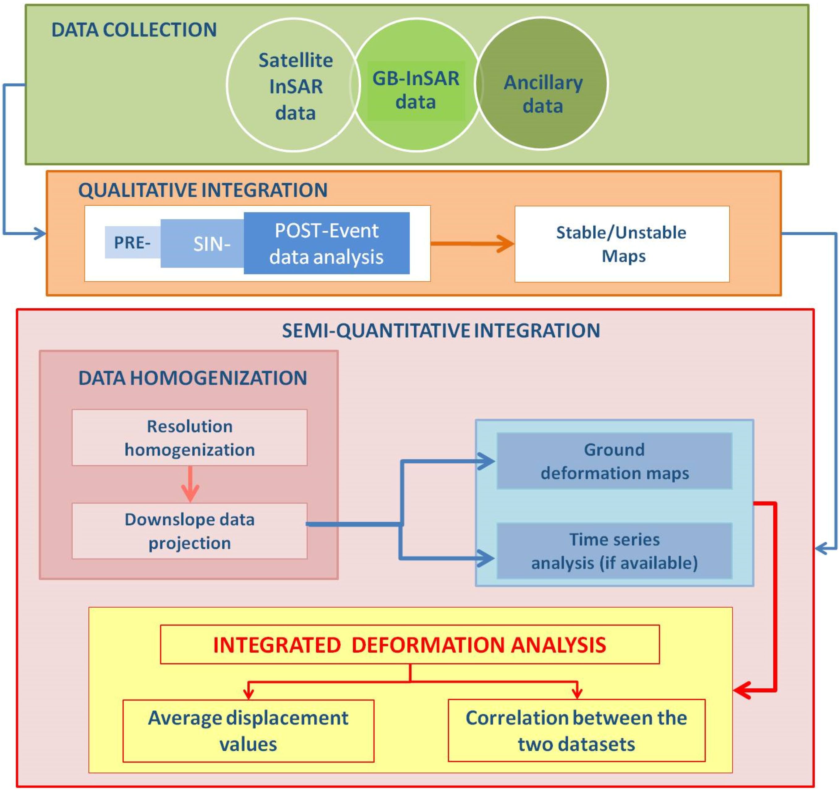
2.1. Data Integration
2.1.1. Qualitative Integration
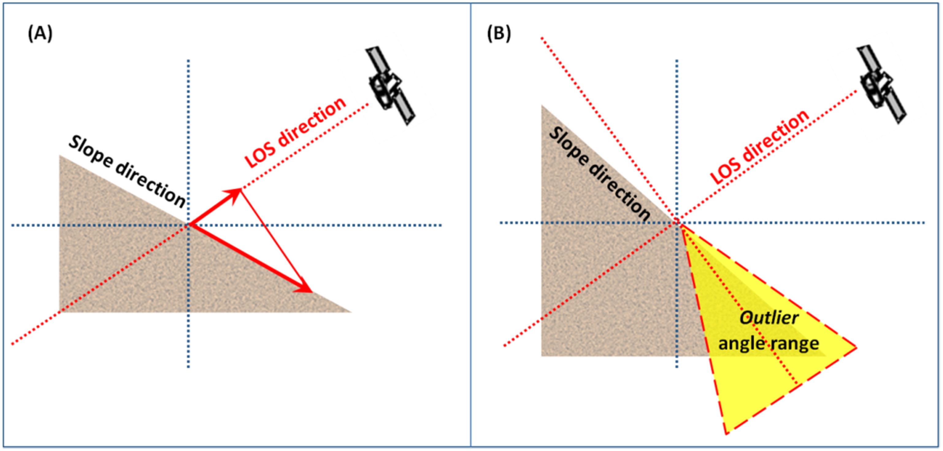
2.1.2. Semi-Quantitative Integration
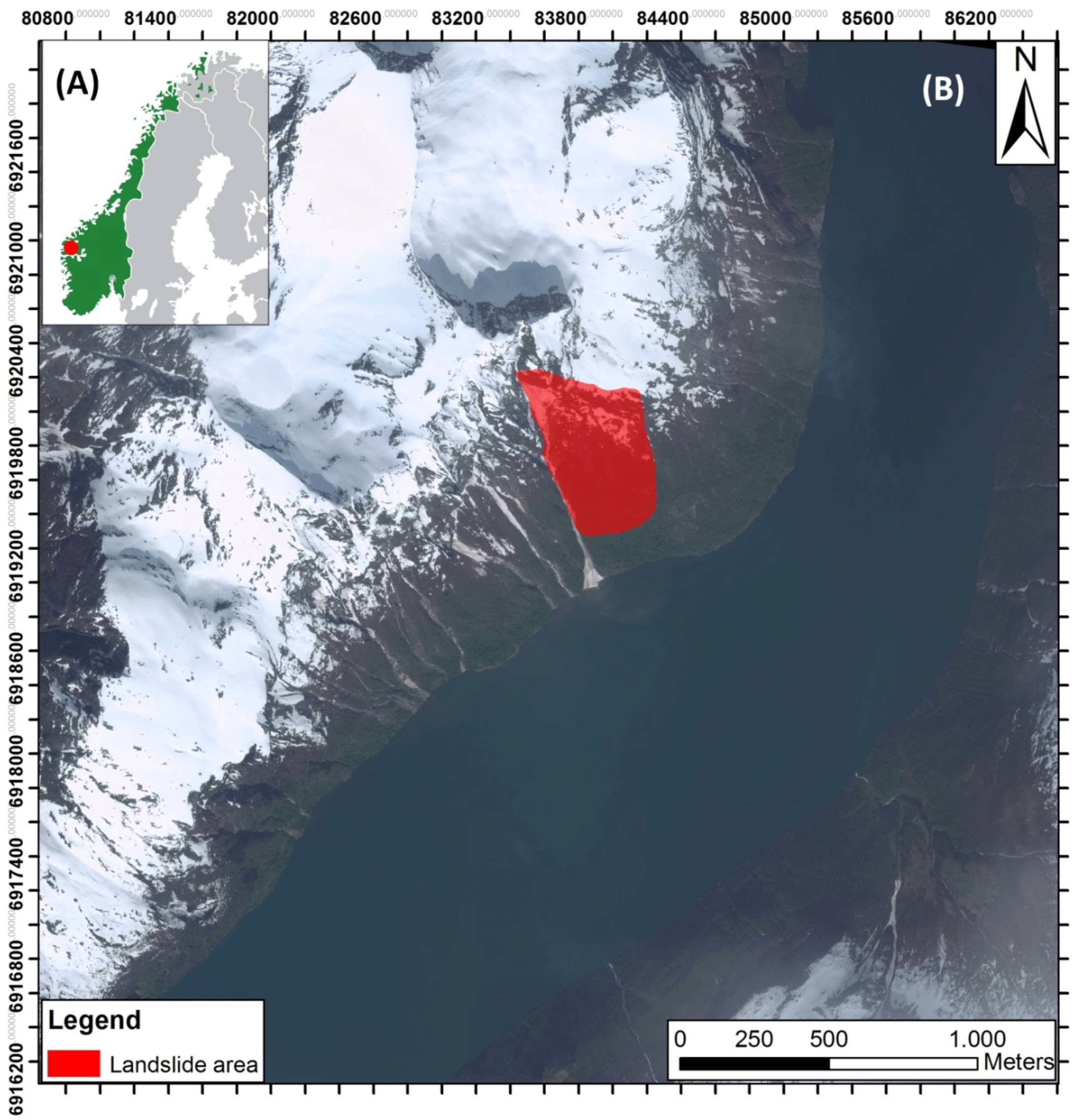
2.2. Åknes Test Site
2.2.1. Location
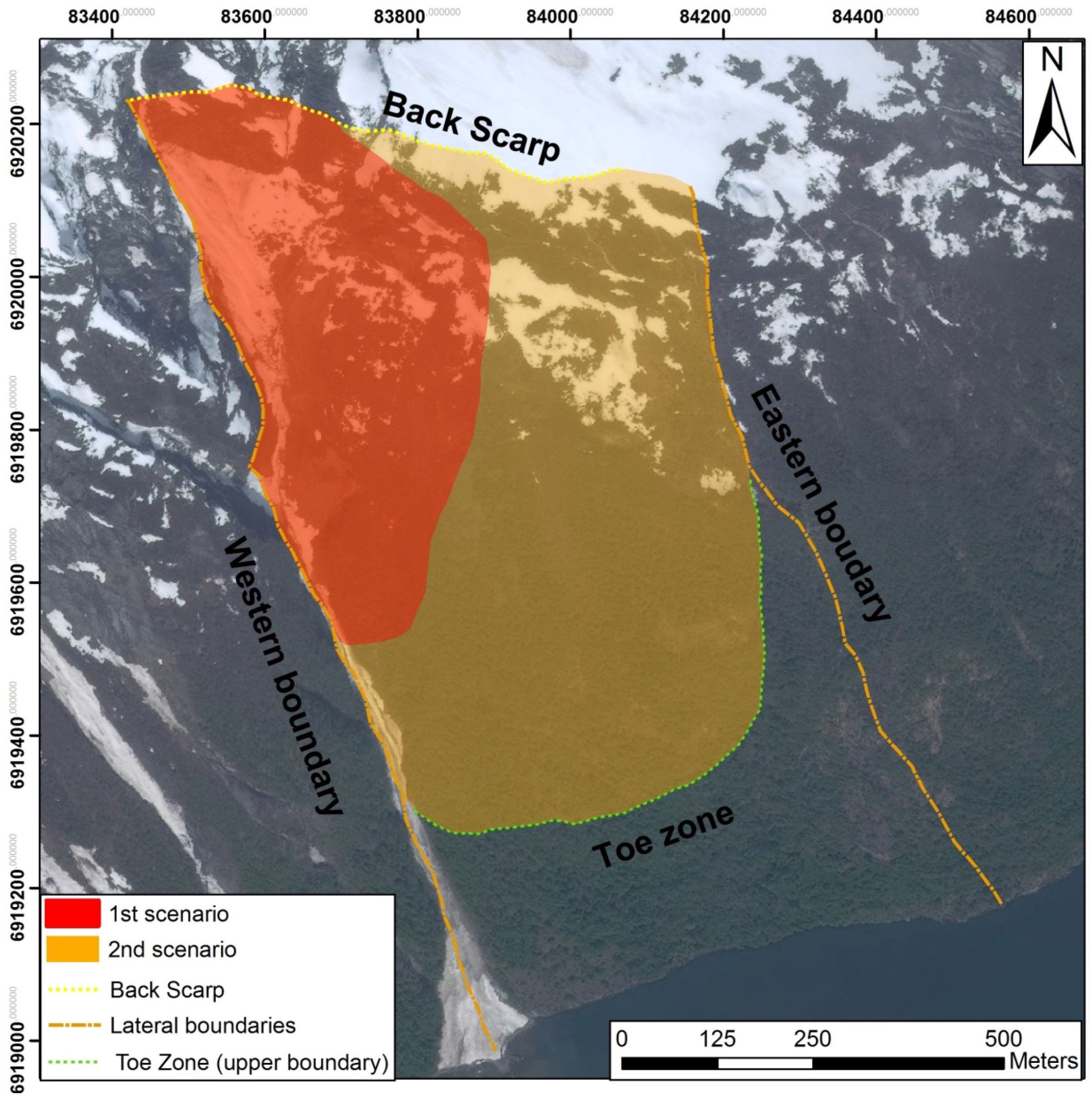
2.2.2. Geological and Geomorphological Setting
2.3. Available Datasets
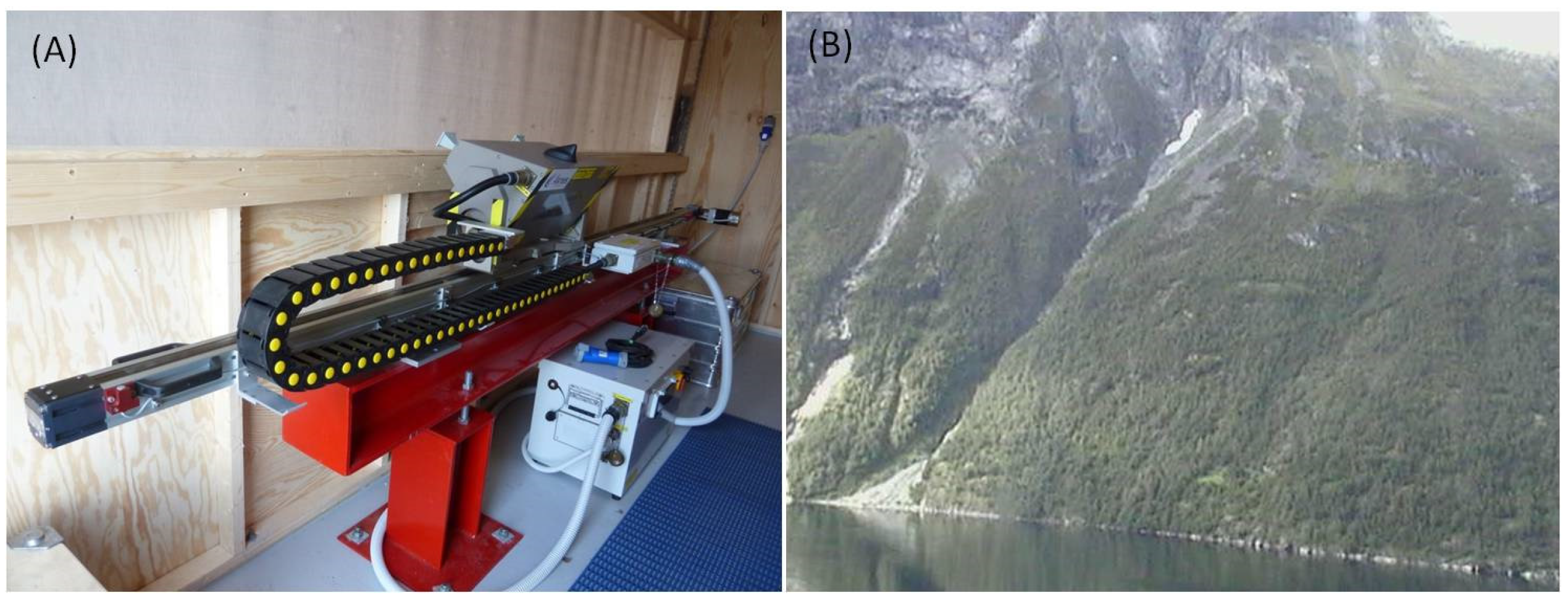
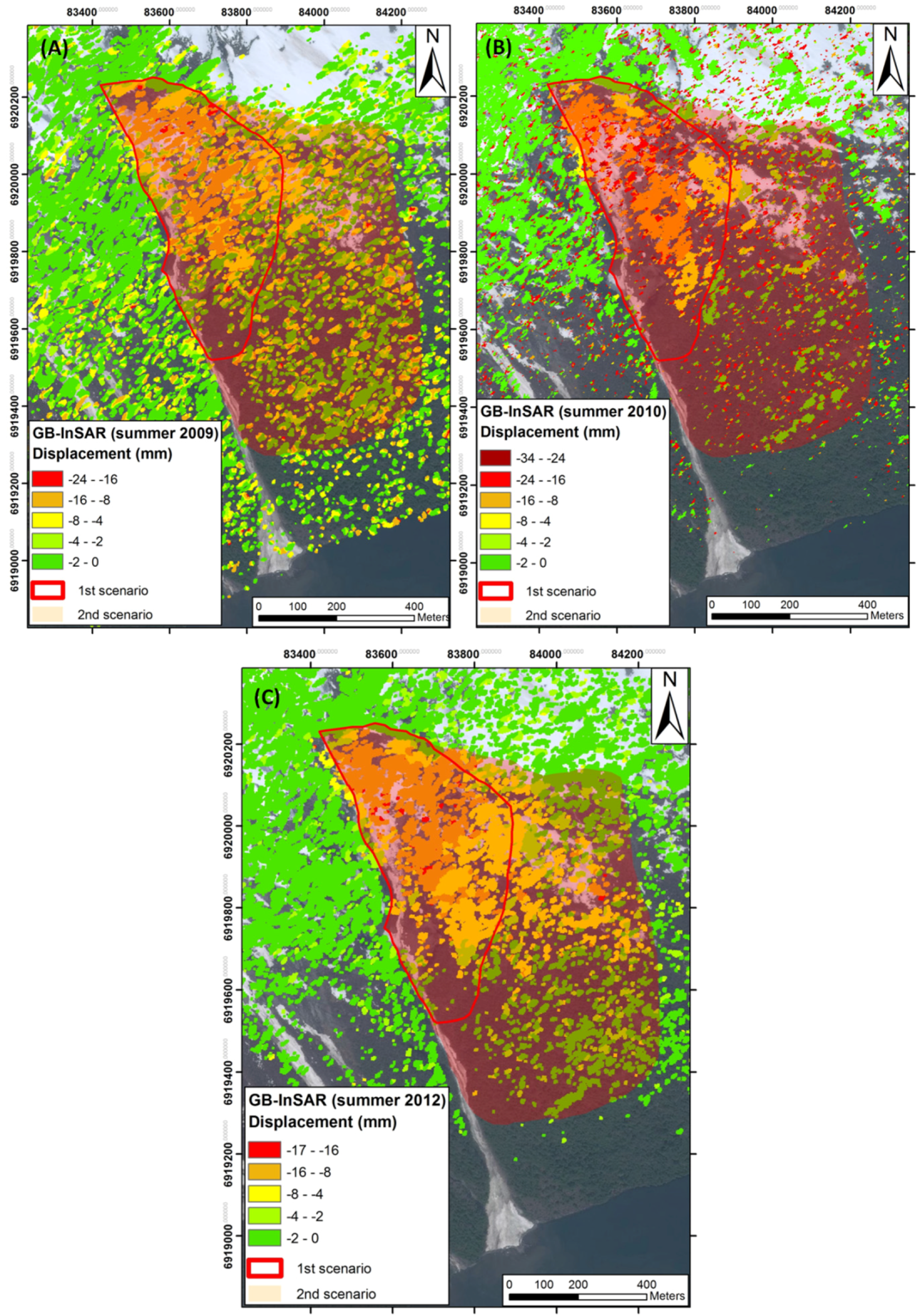
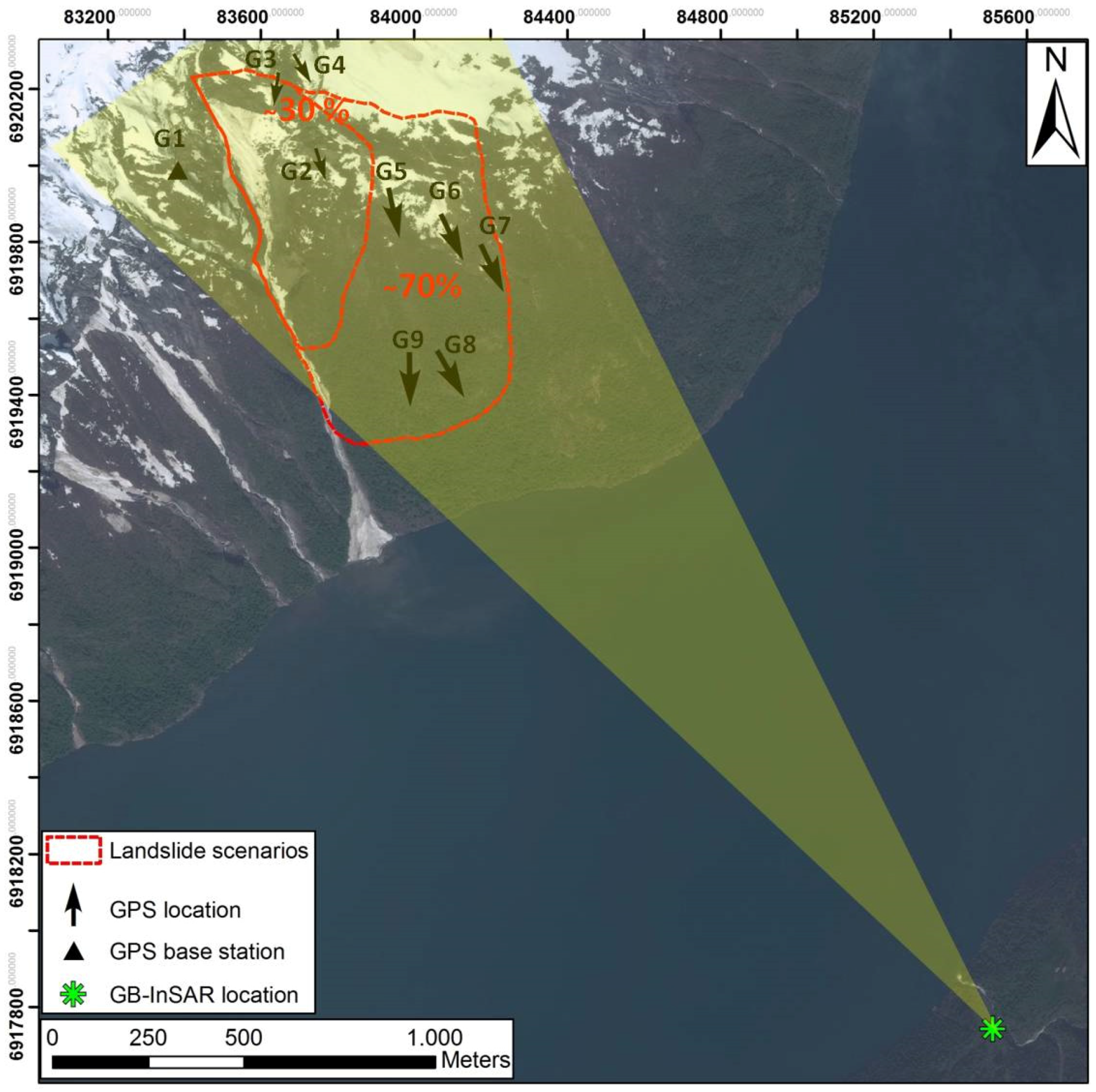
2.3.1. GB-InSAR Monitoring Activity
2.3.2. Satellite InSAR Monitoring Activity
3. Results
3.1. Qualitative Integration Results
3.2. Semi-Quantitative Integration Results
4. Discussion
5. Conclusions
Acknowledgments
Author Contributions
Conflicts of Interest
References
- IGOS (Integrated Global Observing Strategy). GEOHAZARDS Theme Report: For the Monitoring of Our Environment from Space and from Earth. European Space Agency publication, 2004. Available online: http://unesdoc.unesco.org/images/0014/001405/140532eo.pdf (accessed on 9 October 2015).
- Columbia University. Global Landslide Total Economic loss Risk Deciles. 2000, vol.1. Available online: http://sedac.ciesin.columbia.edu/data/set/ndh-landslide-total-economic-loss-risk-deciles (accessed on 9 October 2015).
- Guzzetti, F. Landslide fatalities and evaluation of landslide risk in Italy. Eng. Geol. 2000, 58, 89–107. [Google Scholar] [CrossRef]
- Petley, D.N. The global occurrence of fatal landslides in 2007. Geophys. Res. Abstr. 2008, 10, EGU2008-A-10487. [Google Scholar]
- Schuster, R.L.; Highland, L. Socioeconomic and Environmental Impacts of Landslides in the Western Hemisphere; US Department of the Interior, US Geological Survey: Cartagena, Colombia, 2001.
- Canuti, P.; Casagli, N.; Ermini, L.; Fanti, R.; Farina, P. Landslide activity as a geoindicator in Italy: Significance and new perspectives from remote sensing. Environ. Geol. 2004, 45, 907–919. [Google Scholar] [CrossRef]
- Kjekstad, O.; Highland, L. Economic and social impacts of landslides. In Landslides–Disaster Risk Reduction; Springer: Berlin, Germany; Heidelberg, Germany, 2009; pp. 573–587. [Google Scholar]
- Nadim, F.; Kjekstad, O.; Peduzzi, P.; Herold, C.; Jaedicke, C. Global landslide and avalanche hotspots. Landslides 2006, 3, 159–173. [Google Scholar] [CrossRef]
- Luzi, G.; Pieraccini, M.; Mecatti, D.; Noferini, L.; Guidi, G.; Moia, F.; Atzeni, C. Ground-based radar interferometry for landslides monitoring: Atmospheric and instrumental decorrelation sources on experimental data. IEEE Trans. Geosci. Remote Sens. 2004, 42, 2454–2466. [Google Scholar] [CrossRef]
- Luzi, G. Ground based SAR interferometry: A novel tool for geoscience. In Geoscience and Remote Sensing; New Achievements, InTech; Imperatore, P., Riccio, D., Eds.; 2010; pp. 1–26. Available online: http://www.intechopen.com/articles/show/title/ground-based-sar-interferometry-a-novel-toolfor-geoscience (accessed on 20 May 2015).
- Monserrat, O.; Crosetto, M.; Luzi, G. A review of ground-based SAR interferometry for deformation measurement. ISPRS J. Photogramm. Remote Sens. 2014, 93, 40–48. [Google Scholar] [CrossRef]
- Ferretti, A.; Prati, C.; Rocca, F. Non linear subsidence rate estimation using Permanent Scatterers in differential SAR interferometry. IEEE Trans. Geosci. Remote Sens. 2000, 38, 2202–2212. [Google Scholar] [CrossRef]
- Ferretti, A.; Prati, C.; Rocca, F. Permanent scatterers in SAR interferometry. IEEE Trans. Geosci. Remote Sens. 2001, 39, 8–20. [Google Scholar] [CrossRef]
- Ferretti, A.; Bianchi, M.; Prati, C.; Rocca, F. Higher-order permanent scatterers analysis. Eurasip J. Appl. Signal Process. 2005, 20, 3231–3242. [Google Scholar] [CrossRef]
- Hanssen, R.S. Satellite radar interferometry for deformation monitoring: A priori assessment of feasibility and accuracy. Int. J. Appl. Earth Obs. Geoinform. 2005, 6, 253–260. [Google Scholar]
- Raucoules, D.; Bourgine, B.; Michele, M.; Le Gozannet, G.; Closset, L.; Bremmer, C.; Veldkamp, H.; Tragheim, D.; Bateson, L.; Crosetto, M.; et al. Validation and intercomparison of persistent scatterers interferometry: PSIC4 project results. J. Appl. Geophys. 2009, 68, 335–347. [Google Scholar] [CrossRef]
- Crosetto, M.; Monserrat, O.; Iglesias, R.; Crippa, B. Persistent scatterer interferometry: Potential, limits and initial C- and X-band comparison. Photogramm. Eng. Remote Sens. 2010, 76, 1061–1069. [Google Scholar] [CrossRef]
- Crosetto, M.; Monserrat, O.; Cuevas-Gonzàlez, M.; Devanthèry, N.; Crippa, B. Persistent scatterer interferometry: A review. ISPRS J. Photogramm. Remote Sens. 2015, in press. [Google Scholar]
- Berardino, P.; Fornaro, G.; Lanari, R.; Sansosti, E. A new algorithm for surface deformation monitoring based on small baseline differential SAR interferograms. IEEE Trans. Geosci. Remote Sens. 2002, 40, 2375–2383. [Google Scholar]
- Rudolf, H.; Leva, D.; Tarchi, D.; Sieber, A.J. Mobile and versatile SAR system. In Proceedings of the IEEE 1999 International Geoscience and Remote Sensing Symposium, Hamburg, Germany, 28 June–2 July 1999; pp. 592–594.
- Tarchi, D.; Rudolf, H.; Luzi, G.; Chiarantini, L.; Coppo, P.; Sieber, A.J. SAR interferometry for structural changes detection: A demonstration test on a dam. In Proceedings of the IEEE 1999 International on Geoscience and Remote Sensing Symposium, Hamburg, Germany, 28 June–2 July 1999; pp. 1522–1524.
- Massonnet, D.; Feigl, K.L. Radar interferometry and its application to changes in the Earth’s surface. Rev. Geophys. 1998, 36. [Google Scholar] [CrossRef]
- Singhroy, V.; Mattar, K.E.; Gray, A.L. Landslide characterisation in Canada using interferometric SAR and combined SAR and TM images. Adv. Space Res. 1998, 21, 465–476. [Google Scholar] [CrossRef]
- Crosetto, M.; Monserrat, O.; Cuevas, M.; Crippa, B. Spaceborne differential SAR interferometry: Data analysis tools for deformation measurement. Remote Sens. 2011, 3, 305–318. [Google Scholar] [CrossRef]
- Lauknes, T.R.; Shanker, A.P.; Dehls, J.F.; Zebker, H.A.; Henderson, I.H.C.; Larsen, Y. Detailed rockslide mapping in northern Norway with small baseline and persistent scatterer interferometric SAR time series methods. Remote Sens. Environ. 2010, 114, 2097–2109. [Google Scholar]
- Blikra, L.H. The Åknes rockslide, Norway. In Landslides: Types, Mechanisms and Modeling; Clague, J.J., Stead, D., Eds.; Cambridge University Press: Cambridge, UK, 2012; pp. 323–335. [Google Scholar]
- Bardi, F.; Frodella, W.; Ciampalini, A.; Bianchini, S.; Del Ventisette, C.; Gigli, G.; Fanti, R.; Moretti, S.; Basile, G.; Casagli, N. Integration between ground based and satellite SAR data in landslide mapping: The San Fratello case study. Geomorphology 2014, 223, 45–60. [Google Scholar] [CrossRef]
- Tofani, V.; Del Ventisette, C.; Moretti, S.; Casagli, N. Integration of remote sensing techniques for intensity zonation within a landslide area: A case study in the northern Apennines, Italy. Remote Sens. 2014, 6, 907–924. [Google Scholar] [CrossRef]
- Eriksen, H.Ø.; Lauknes, T.R.; Larsen, Y.; Dehls, J.F.; Grydeland, T.; Bunkholt, H. Satellite and Ground-Based Interferometric Radar Observations of an Active Rockslide in Northern Norway. In Engineering Geology for Society and Territory; Springer International Publishing: Cham, Switzerland, 2015; pp. 167–170. [Google Scholar]
- Zebker, H.A.; Villasenor, J. Decorrelation in interferometric radar echoes. IEEE Trans. Geosci. Remote Sens. 1992, 30, 950–959. [Google Scholar] [CrossRef]
- Cruden, D.M.; Varnes, D.J. Landslide types and processes. In Landslides: Investigation and Mitigation; Transportation Research Board, Special Report, 247; Turner, A.K., Schuster, R.L., Eds.; Transportation Research Board, National Research Council, National Academy Press: Washington, DC, USA, 1996; pp. 36–75. [Google Scholar]
- Raspini, F.; Ciampalini, A.; Del Conte, S.; Lombardi, L.; Nocentini, M.; Gigli, G.; Ferretti, A.; Casagli, C. Exploitation of amplitude and phase of satellite SAR images for landslide mapping: the case of Montescaglioso (South Italy). Remote Sens. 2015, 7, 14576–14596. [Google Scholar] [CrossRef]
- Bianchini, S.; Cigna, F.; Righini, G.; Proietti, C.; Casagli, N. Landslide hotspot mapping by means of persistent scatterer interferometry. Environ. Earth. Sci. 2012, 67, 1155–1172. [Google Scholar] [CrossRef]
- Lauknes, T.R. Rockslide Mapping in Norway by Means of Interferometric SAR Time Series Analysis. Ph.D. Thesis, University of Trømso (UIT), Trømso, Norway, 2010. [Google Scholar]
- Intrieri, E.; Gigli, G.; Mugnai, F.; Fanti, R.; Casagli, N. Design and implementation of a landslide early warning system. Eng. Geol. 2012, 147–148, 124–136. [Google Scholar] [CrossRef]
- Ciampalini, A.; Bardi, F.; Bianchini, S.; Frodella, W.; Del Ventisette, C.; Moretti, S.; Casagli, N. Analysis of building deformation in landslide area using multisensor PSInSAR technique. Int. J. Appl. Earth Obs. Geoinform. 2014, 33, 166–180. [Google Scholar] [CrossRef]
- Bovenga, F.; Wasowski, J.; Nitti, D.O.; Nutricato, R.; Chiaradia, M.T. Using COSMO SkyMed X-band and ENVISAT C-band SAR interferometry for landslides analysis. Remote Sens. Environ. 2012, 119, 272–285. [Google Scholar] [CrossRef]
- Wright, T.J.; Parsons, B.E.; Lu, Z. Toward mapping surface deformation in three dimensions using InSAR. Geophys. Res. Lett. 2004, 31, L010607. [Google Scholar] [CrossRef]
- Tofani, V.; Raspini, F.; Catani, F.; Casagli, N. Persistent Scatterer Interferometry (PSI) technique for landslide characterization and monitoring. Remote Sens. 2013, 5, 1045–1065. [Google Scholar] [CrossRef]
- Colesanti, C.; Wasowski, J. Investigating landslides with space-borne Synthetic Aperture Radar (SAR) interferometry. Eng. Geol. 2006, 88, 173–199. [Google Scholar] [CrossRef]
- Cascini, L.; Fornaro, G.; Peduto, D. Advanced low- and full-resolution DInSAR map generation for slow-moving landslide analysis at different scales. Eng. Geol. 2010, 112, 29–42. [Google Scholar] [CrossRef]
- Herrera, G.; Gutiérrez, F.; Garcìa-Davalillo, J.C.; Guerrer, J.; Notti, D.; Galve, J.P.; Fernàndez-Merodo, J.A.; Cooksley, G. Multi-sensor advanced DInSAR monitoring of very slow landslides: The Tena Valley case study (Central Spanish Pyrenees). Remote Sens. Environ. 2013, 128, 31–43. [Google Scholar] [CrossRef]
- Barbieri, M.; Corsini, A.; Casagli, N.; Farina, P.; Coren, F.; Sterzai, P.; Leva, D.; Tarchi, D. Space-Borne and Ground-Based SAR Interferometry for Landslide Activity Analysis and Monitoring in the Appennines of Emilia Romagna (Italy): Review of Methods and Preliminary Results; European Space Agency, (Special Publication): Noordwijk, The Netherlands, 2004; pp. 463–470. [Google Scholar]
- Ganerød, G. V.; Grøneng, G.; Rønning, J. S.; Dalsegg, E.; Elvebakk, H.; Tønnesen, J. F.; Kveldsvik, V.; Eiken, T.; Blikra, L. H.; Braathen, A. Geological model of the Åknes rockslide, western Norway. Eng. Geol. 2008, 102, 1–18. [Google Scholar] [CrossRef]
- Blikra, L.H.; Braathen, A.; Derron, M.H.; Eiken, T.; Kveldsvik, V.; Grøneng, G.; Dalsegg, E.; Elvebakk, H.; Roth, M. The Åkerneset slope failure—A potential catastrophic rockslide in western Norway? Abstr. Proc. Geol. Soc. Nor. 2005, 1, 15–16. [Google Scholar]
- Eidsvik, U.M.; Medina-Cetina, Z.; Kveldsvik, V.; Glimsdal, S.; Harbitz, C.B.; Sandersen, F. Risk assessment of a tsunamigenic rockslide at Åknes. Nat. Hazards 2011, 56, 529–545. [Google Scholar] [CrossRef]
- Tveten, E.; Lutro, O.; Thorsnes, T. Geologisk kart over Norge, bergrunnskart Ålesund, 1:250,000, (Ålesund, Western Norway); Geological Survay of Norway: Trondheim, Norway, 1988. (In Norwegian) [Google Scholar]
- Heincke, B.; Gunther, T.; Dalsegg, E.; Ronning, J.S.; Ganerød, G.V.; Elvebakk, H. Combined three-dimensional electric and seismic tomography study on the Aknes rockslide in western Norway. J. Appl. Geophys. 2010, 70, 292–306. [Google Scholar] [CrossRef] [Green Version]
- Kristensen, L.; Rivolta, C.; Dehls, J.; Blikra, L.H. GB-InSAR measurement at the Åknes rockslide, Norway. In Proceedings of the International Conference Vajont 1963–2013. Thoughts and Analyses after 50 Years since the Catastrophic Landslide, Padua, Italy, 8–10 October 2013.
- Frei, C. H.; Loew, S.; Leuenberger-West, F. First results of a large-scale multi-tracer test within an unstable rockslide area (Åknes, Norway). Geophys. Res. Abstr. 2008, 10. SRef-ID:1607-7962/gra/EGU2008-A-08930. [Google Scholar]
- Kveldsvik, V.; Nilsen, B.; Einstein, H.H.; Nadim, F. Alternative approaches for analyses of a 100,000 m3 rock slide based on Barton-Bandis shear strength criterion. Landslides 2007, 5, 161–176. [Google Scholar] [CrossRef]
- Kveldsvik, V.; Kanya, A.M.; Nadim, F.; Bhasin, R.; Nilsen, B.; Einstein, H.H. Dynamic distinct-element analysis of the 800 m high Aknes rock slope. Int. J. Rock Mech. Min. Sci. 2009, 46, 686–698. [Google Scholar] [CrossRef]
- Kveldsvik, V.; Einstein, H.H.; Nilsen, B.; Blikra, L.H. Numerical analysis of the 650,000 m2 Aknes rock slope based on measured displacements and geotechnical data. Rock. Mech. Rock. Eng. 2009, 42, 689–728. [Google Scholar] [CrossRef]
- Nordvik, T.; Nyrnes, E. Statistical analysis of surface displacements—An example from the Åknes rockslide, western Norway. Nat. Hazards Earth. Syst. Sci. 2009, 9, 713–724. [Google Scholar] [CrossRef] [Green Version]
- Blikra, L.H. The Åknes rockslide: Monitoring, threshold values and early-warning. In Proceedings of the 10th International Symposium on Landslides and Engineered Slopes, Xian, China, 30 June–4 July 2008; pp. 1089–1094.
- Lacasse, S.; Eidsvig, U.; Nadim, F.; Hoeg, K.; Blikra, L.H. Evaluation of Åknes rockslide hazard using event trees. In Proceedings of the 42nd U.S. Rock Mechanics Symposium (USRMS), ARMA-08-340, San Francisco, CA, USA, 29 June–2 July 2008.
- The Norwegian Water Resources and Energy Directorate (NVE). Available online: http://www.nve.no/english/ (accessed on 12 March 2015).
- Tarchi, D.; Casagli, N.; Fanti, R.; Leva, D.; Luzi, G.; Pasuto, A.; Pieraccini, M.; Silvano, S. Landslide monitoring by using ground-based SAR interferometry: An example of application to the Tessina landslide in Italy. Eng. Geol. 2003, 1, 15–30. [Google Scholar] [CrossRef]
- Northern Research Institute of Trømso (NORUT) (Trømso, Norway). Unpublished work. 2013.
- Hooper, A.; Zebker, H.A.; Segall, P.; Kampes, B. A new method for measuring deformation on volcanoes and other natural terrains using InSAR persistent scatterers. Geophys. Res. Lett. 2004, 31, 1–5. [Google Scholar] [CrossRef]
- Lauknes, T.R.; Zebker, H.A.; Larsen, L. InSAR deformation time series using an L1-Norm small-baseline approach. IEEE Trans. Geosci. Remote Sens. 2011, 49, 536–546. [Google Scholar] [CrossRef]
- Lillesand, T.M.; Kiefer, R.W.; Chipman, J.W. Remote sensing and Image Interpretation, 5th ed.; Wiley, Cop.: New York, NY, USA, 2004. [Google Scholar]
- Raspini, F.; Moretti, S.; Fumagalli, A.; Rucci, A.; Novali, F.; Ferretti, A.; Prati, C.; Casagli, N. The COSMO-SkyMed constellation monitors the costa concordia wreck. Remote Sens. 2014, 6, 3988–4002. [Google Scholar] [CrossRef] [Green Version]
- Ciampalini, A.; Raspini, F.; Bianchini, S.; Tarchi, D.; Vespe, M.; Moretti, S.; Casagli, N. The costa concordia last cruise: The first application of high frequency monitoring based on COSMO-SkyMed constellation for wreck removal. J. Photogramm. Remote Sens. 2016. [Google Scholar] [CrossRef]


| GB-InSAR Campaigns |
|---|
| 21 July 2006–25 October 2006 |
| 17 July 2008–13 October 2008 |
| 1 July 2009–17 October 2009 |
| 9 July 2010–31 October 2010 |
| 12 July 2012–24 October 2012 |
| GB-InSAR | |
|---|---|
| Rail length | 3 m |
| Central frequency | 17.2 GHz |
| Bandwidth | 60 MHz |
| Number of frequencies | 2501 |
| Steps along the rail | 601 |
| Image acquisition time | 8 min |
| Processed image range | 1800–4200 m |
| Processed image azimuth | ±1200 m |
| Distance to the back scarp | 3000 m |
| GPS Stations | GPS 3D Movement | Displacement Registered by GB-InSAR at GPS Location | LOS % of True Vector |
|---|---|---|---|
| G2 | 85.1 mm/y | 30 mm/y | 35% |
| G3 | 81.4 mm/y | 24 mm/y | 29% |
| G4 | 2.8 mm/y | 1 mm/y | 30% |
| G5 | 30.6 mm/y | 20 mm/y | 66% |
| G6 | 17.6 mm/y | 13 mm/y | 73% |
| G7 | 25.8 mm/y | 19 mm/y | 75% |
| G8 | 14.7 mm/y | 10 mm/y | 71% |
| G9 | 4.9 mm/y | 3 mm/y | 63% |
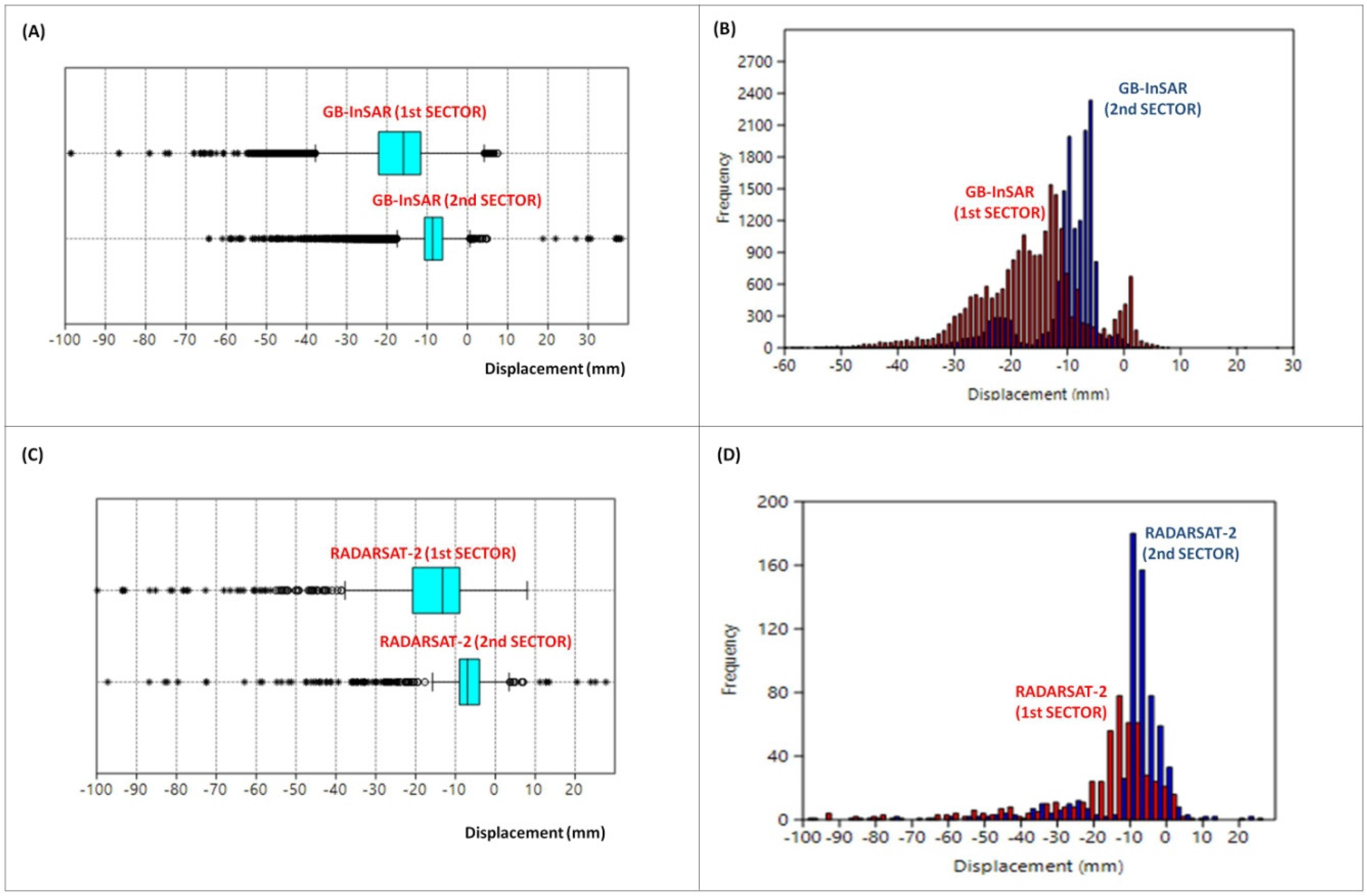
| GB-InSAR (1st Sector) | GB-InSAR (2nd Sector) | RADARSAT-2 (1st Sector) | RADARSAT-2 (2nd Sector) | |
|---|---|---|---|---|
| Mean | −17 mm | −10 mm | −18 mm | −9 mm |
| Median | −16 mm | −9 mm | −13 mm | −7 mm |
| SD | 10 | 7 | 17 | 13 |
| 25 Percentile | −22 mm | −11 mm | −21 mm | −9 mm |
| 75 Percentile | −12 mm | −6 mm | −9 mm | −4 mm |
© 2016 by the authors; licensee MDPI, Basel, Switzerland. This article is an open access article distributed under the terms and conditions of the Creative Commons by Attribution (CC-BY) license (http://creativecommons.org/licenses/by/4.0/).
Share and Cite
Bardi, F.; Raspini, F.; Ciampalini, A.; Kristensen, L.; Rouyet, L.; Lauknes, T.R.; Frauenfelder, R.; Casagli, N. Space-Borne and Ground-Based InSAR Data Integration: The Åknes Test Site. Remote Sens. 2016, 8, 237. https://0-doi-org.brum.beds.ac.uk/10.3390/rs8030237
Bardi F, Raspini F, Ciampalini A, Kristensen L, Rouyet L, Lauknes TR, Frauenfelder R, Casagli N. Space-Borne and Ground-Based InSAR Data Integration: The Åknes Test Site. Remote Sensing. 2016; 8(3):237. https://0-doi-org.brum.beds.ac.uk/10.3390/rs8030237
Chicago/Turabian StyleBardi, Federica, Federico Raspini, Andrea Ciampalini, Lene Kristensen, Line Rouyet, Tom Rune Lauknes, Regula Frauenfelder, and Nicola Casagli. 2016. "Space-Borne and Ground-Based InSAR Data Integration: The Åknes Test Site" Remote Sensing 8, no. 3: 237. https://0-doi-org.brum.beds.ac.uk/10.3390/rs8030237