A Stochastic Geometry Method for Pylon Reconstruction from Airborne LiDAR Data

Abstract

Object detection and reconstruction from remotely sensed data are active research topic in photogrammetric and remote sensing communities. Power engineering device monitoring by detecting key objects is important for power safety. In this paper, we introduce a novel method for the reconstruction of self-supporting pylons widely used in high voltage power-line systems from airborne LiDAR data. Our work constructs pylons from a library of 3D parametric models, which are represented using polyhedrons based on stochastic geometry. Firstly, laser points of pylons are extracted from the dataset using an automatic classification method. An energy function made up of two terms is then defined: the first term measures the adequacy of the objects with respect to the data, and the second term has the ability to favor or penalize certain configurations based on prior knowledge. Finally, estimation is undertaken by minimizing the energy using simulated annealing. We use a Markov Chain Monte Carlo sampler, leading to an optimal configuration of objects. Two main contributions of this paper are: (1) building a framework for automatic pylon reconstruction; and (2) efficient global optimization. The pylons can be precisely reconstructed through energy optimization. Experiments producing convincing results validated the proposed method using a dataset of complex structure.

1. Introduction

Object extraction and reconstruction from remotely sensed data has been a motivating topic for many researchers in the past years. Indeed, 3D models can be very useful in various applications such as urban planning, navigation, and emergency response.

Power-line systems convey electric energy between networks of electric facilities to provide electricity to millions of homes and business. Monitoring of power lines is traditionally labor intensive [1,2,3]. Automating the monitoring of high-voltage transmission line systems is of importance to power utility safety [4,5]. Pylons, which support the heavy power lines and resist the force of side winds, are very important components for power-line systems. The importance of the 3D reconstruction of pylons is two-fold: (1) constructing information systems for pylons and other electric facilities can be helpful for construction planning; and (2) through reconstruction, we can obtain the accurate positions and parameters of pylons, which is important information for electrical safety applications such as disaster recovery and radiation testing of high-voltage power [6]. Therefore, a good knowledge of the pylon types and parameters are of great importance to all local communities for disaster management, urban planning, environmental protection, and urban development policy planning.

Laser scanning can directly provide 3D point cloud data, which is more advanced than other remotely sensed data (e.g., remote sensing images), for the modeling of complex objects. In 2002, an on-board eye-safe laser radar system capable of measuring the distance between high-voltage power transmission lines and nearby trees was developed [4]. In power-line system surveying, dense points on power lines and pylons can now be accurately measured using laser scanning [7,8].

This paper focuses on the problem of pylon reconstruction using airborne LiDAR. We first automatically extract the pylon points from the dense point cloud data. The pylons are then automatically modeled using a model-based method. Based on the regularity of the construction, pylons that support power lines may be of similar types, but have different sizes and heights. In some situations, the pylons along a single power line may even be of different types in order to adapt to the changing of topography. Therefore, determining the types and fitting the parameters are two important tasks in the reconstruction. The most recent work has focused on reconstruction from remotely sensed data, which requires heavy user interaction [6]. However, this method is not practical for most field research because it is too labor-intensive. Thus, it is necessary to develop a rapid, robust, and reliable methodology for the automatic reconstruction of pylons. We focus on pylons for the 220–500 kV power systems common in China, as ultrahigh-voltage power systems are still in development in China. The ultrahigh-voltage pylons are, however, similar to those used for lower voltages. Thus, the reconstruction method proposed in this paper could be adapted to future systems.

1.1. Related Work

A tremendous variety of approaches exist in the literature for 3D object reconstruction. However, there have been very few studies of the automatic reconstruction of pylons. Li et al. introduced a model-based pylon reconstruction method [9]. In that model, a pylon is precisely reconstructed by being divided into legs, body and head. However, this method is not suitable for automatic pylon reconstruction in large areas by introducing many steps and interactive operation. Therefore, we mainly consider the literature about automatic reconstruction of objects, which has been widely researched (e.g., building and tree). The approaches about 3D object reconstruction relevant to our work are discussed in the following sections.

3D Object Reconstruction

There has been very little research into the problem of pylon modeling. To date, power-related object reconstruction has mainly focused on power lines [10,11,12]. Pylons are man-made objects with constructing specification; therefore, we mainly refer to the reconstruction of objects with regularity (such as buildings). Besides the regular objects, some mostly researched irregular objects (such as trees) are also referenced to develop effective methods. To model objects, data-driven and model-driven methods are the two commonly applied solutions.

(1) Data-driven methods 

Data-driven methods are mainly based on combining several kinds of primitives of objects. Pylons are constructed out of a main frame and arms. Therefore, a pylon could be reconstructed using data-driven methods.

Buildings are constructed with primitives such as 3D-lines, planes, and facades. Much work detailing building reconstruction by combining such primitives has been published. Maas and Vosselman reconstructed buildings using a polyhedral model by first detecting planar faces. The outlines of roof faces were then reconstructed by intersection of the corresponding planes [13]. Frueh et al. used laser scans to model buildings with a detailed reconstruction of the facades [14]. Taillandier and Deriche used a generic Bayesian framework to model buildings as polyhedral shapes with no overhang by combining base plane primitives [15].

Tree primitives contain wood and foliage components. Côté et al. first extracted vital clues to the main branching structure of the tree (the shape of the trunk and the main branches). They then used that skeleton to add other branches at locations where the presence of foliage was very likely. Finally, they iteratively used the availability of light as a criterion to add foliage in the center of the crown where LiDAR information was sparse or absent due to occlusion effects [16].

These data-driven methods can provide accurate descriptions of common objects. However, they are not suited to the modeling of large scenes since they usually demand high-resolution data and require very lengthy computation times.

(2) Model-driven reconstruction methods 

Model-based methods can be used to reconstruct objects with constant parameters or construction rules. These methods are known to be robust with respect to data quality, and are suited to large scenes. As for power lines, McLaughlin defined the parameters of a model, and extracted each individual transmission line span from classified power-line point cloud data [11]. Based on RANdom SAmple Consensus (RANSAC) rule, Guo et al. proposed an improved approach for power-line modeling [17].

Buildings are constructed with certain models. Brédif et al. presented a method including parametric roof superstructure reconstruction using a Minimum Description Length energy minimization [18]. Lafarge et al. proposed an approach based on a structural concept: reconstructing buildings by assembling simple urban structures [19].

Livny et al. used the properties of tree skeletal structures to construct a Branch-Structure Graph [20]. Through global optimization, skeletal structures can be fitted from the often sparse, incomplete, and noisy point cloud data.

The main merit of the model-based reconstruction methods is their insensitivity to data loss by imposing constraints on the model’s parameters and construction rules. Since the pylons are elements that follow a power industry standard of a limited number of shape types, the model-driven methods are a more suitable solution for this type of model reconstruction.

1.2. Motivation and Contributions

In this paper, we propose an automatic high-precision method for pylon reconstruction from airborne LiDAR data. Given the construction regularity of pylons, the model-based method is mainly used in order to avoid labor-intensive work to determine the types and fitting the parameters. We transform the reconstruction process to be an energetic formulation that states the problem as a minimization of a function mainly made up of data attachments of the measured data and object configurations. In this reconstruction process, the type and parameters of a pylon are simultaneously fitted.

This approach is particularly interesting since it has certain advantages:

(1) In power engineering, pylons are built with regularity that can be parameterized. Parameterized models can provide important semantic knowledge, e.g., the height of pylons and the length of arms. In this way, an efficient library can be generated as objects, which are defined by the parameter sets. This approach therefore guarantees the robustness of the reconstruction by introducing the regularity, which can overcome the defaults of reconstruction errors due to tiny data loss.

(2) The method used in this paper is insensitive to data loss. There is much sparsity and occlusion in LiDAR datasets due to low reflectivity or the blocking out of laser scanning. Model-based reconstruction can be used to overcome these data flaws, to some extent, based on the inherent information (e.g., regularity and symmetry) provided by the models.

The main contributions of the proposed method are as follows:

(1) A framework for automatic pylon reconstruction.

As previously mentioned, automatic pylon reconstruction has not previously been explored in depth, and previous attempts at pylon reconstruction have mainly involved labor-intensive user interaction. Based on the automatic classification of point cloud data into different target types, we first precisely extract pylons using a graph-cut approach and power-line contextual error elimination. A model-based method is then introduced for the pylon reconstruction. The reconstruction is based on stochastic geometry by building an energy function including the data coherence term and the regularization term (Section 3.3). By minimizing the energy function, pylons can be reconstructed.

(2) Efficient global optimization.

Our problem lies in a high-dimensional space of unknown dimensions, and is also non-convex. The sampling of the objective energy function is conducted thanks to a Markov Chain Monte Carlo (MCMC) sampler and is coupled with simulated annealing to find its optimum. This global optimization is well adapted to our case as it finds the minimum of the energy function without becoming trapped in local minima. It also allows us to find an optimal configuration of objects without any initialization prior on the object configuration.

1.3. Overview

The rest of this paper is organized as follows. Before reconstruction, the pylon points have to be extracted from the original point cloud data using a classification method, which is briefly presented in Section 2. In Section 3, we give the essential details of pylon reconstruction. Test area and data characteristics are given in Section 4. Section 5 presents the extensive experimental results with a complex dataset. The reconstruction errors are discussed in Section 6. Finally, we present the conclusions in Section 7.

2. Extraction of Pylon Points

2.1. Classification of Point Cloud Data Based on JointBoost

Before reconstruction, laser points of target objects must be extracted from the point cloud data using a classification method. There are two approaches to classification point cloud data. One approach is to directly extract points of target objects, such as terrain [21], building [22] and vegetation [23,24]. The second approach is to classify all the points into different classes that contain the target types [8,25,26]. The first approach is effective; however, outliers are difficult to eliminate due to the fact that all the other types of points are labeled as noise points. The second approach can provide the contextual information for classes that are helpful for the precise object extraction. Because very few studies have specifically dealt with pylon extraction, we refer to general classification methods of point cloud data [7]. The contextual information is then used to eliminate errors.

The point cloud data are automatically classified into five classes: ground, vegetation, building, power line, and pylon. Classifying the dataset into five classes can be used to eliminate pylon extraction errors by post processing (Section 2.2). We use the approach described in our previous work [7] for the point cloud classification. Firstly, 26 features based on the geometry and echo information of the point cloud are calculated. Based on the calculated features, the JointBoost classifier [27] is used to classify the point cloud into different target classes. The JointBoost classifier is a multi-class boosting machine learning algorithm which can handle a large number of input features for multi-class classification. JointBoost is a special boosting algorithm designed to share features among classes and use fewer features than other classifiers. Moreover, the JointBoost has the capacity to automatically select useful features by minimizing a cost function. Therefore, we applied JointBoost for feature selection and airborne LiDAR point cloud classification. A typical classification result for a pylon is shown in Section 5. However, it can be seen that there are many outlier errors in the classification result. In order to guarantee reconstruction quality, post-processing must be performed to precisely extract the pylons.

2.2. Post-Processing

2.2.1. Graph Cut for Pylon Extraction

For precise pylon extraction, we adopt techniques from computer vision and computer graphics, where the graph-cut approach is employed to separate an object of interest from its background in the data [28].

The two key points of graph cut are: (1) foreground and background seed point selection; and (2) graph building. A region growing algorithm is first used to cluster nearby points with the same initial classification labels. We consider groups with a large number of clustered points to be reliable, while ones with a very small number are considered to be unreliable. The thresholds for reliable groups of each class are determined using a training dataset. For graph cut of a pylon, the seeds of foreground are points that belong to the reliable pylon group. The seeds of background are points that belong to reliable groups of other kinds besides pylon. In the graph building, edges are constructed with a k-nearest neighbor system for the input points. The edges have weights that decrease with distance. In this way, the closer points are more strongly connected than the other points. Further details of the graph-cut approach can be found in our previous work [7].

2.2.2. Classification Outlier Elimination

In the intersection regions between power lines and pylons, many non-pylon points are misclassified as pylons and cannot be distinguished by graph cut. These errors greatly affect the reconstruction quality. We first extract the power lines [11] and determine the intersection points between the power lines and the main plane of the pylons in order to find areas where outliers exist. The points close to these intersection points with a low density are considered to be non-pylon points. In order to detect these points, a projection method is introduced. We first construct projection planes around the intersection points of the power lines and pylons. A projection plane is then sliced into many bins. The bins with few points or short lengths are determined to be non-pylon points. The details are described in Section 5.1.2.

3. 3D Reconstruction

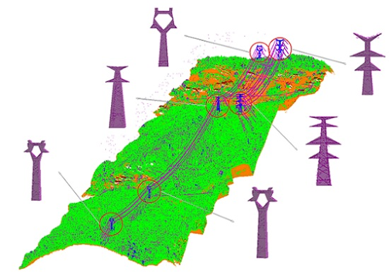
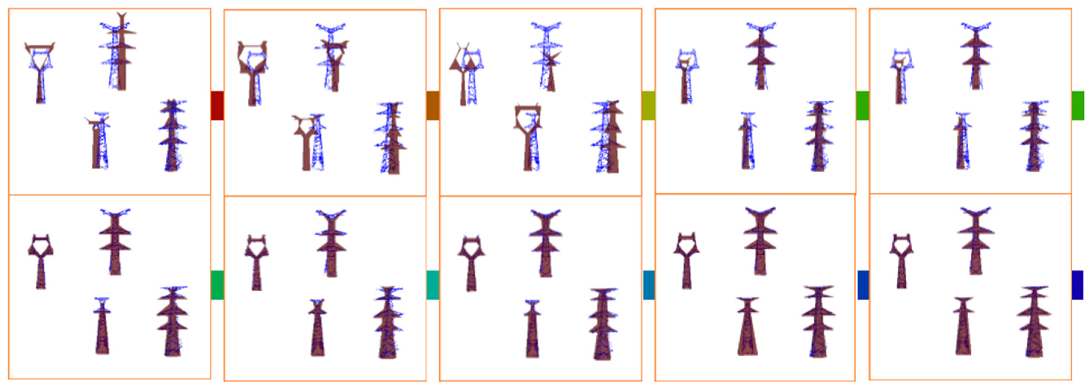
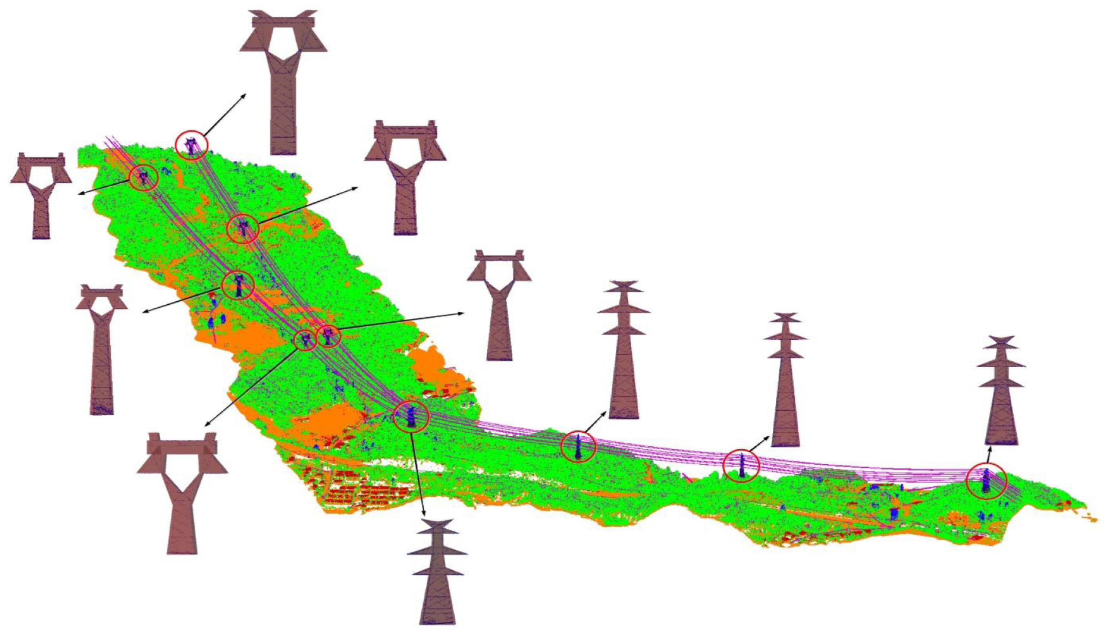
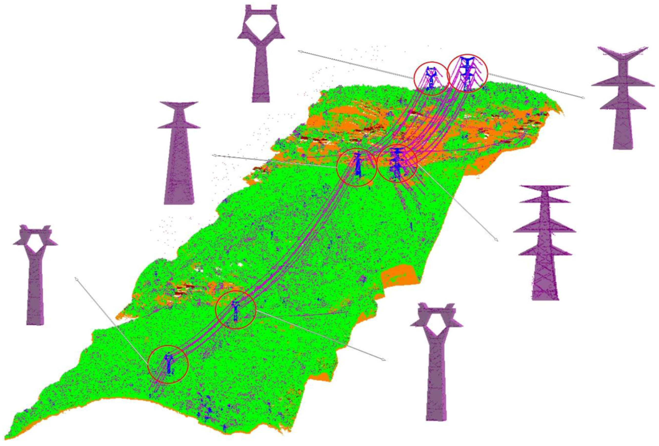
Once the pylon points have been extracted, the models are automatically reconstructed through an optimization method. The first step consists of specifying the 3D objects, which are represented by parameter sets. An energy formulation is then built to measure the coherence degree of the objects and extracted points. Finally, an MCMC method combining simulated annealing is used to optimize the energy formulation in order to find the optimal parameters of pylons. The pylons are constructed with regularity, thus we use a model-based method to reconstruct pylons. As seen in Figure 1, the number of arms of different pylons is different. However, with different positions of arms and various pylons with same number arms, only fitting the number of arms is not sufficient for precise reconstruction of pylons.

3.1. Library of 3D Objects

Pylons are constructed with regularity. The first step of the 3D reconstruction consists of specifying the 3D object models. We refer to the specification widely used in China for pylon construction.

The content of the library $\mathcal{M}$ is a very important thing: if it is too limited, the method loses generality. In this library, there are many of the common self-supporting pylons used in 220–500 kV power-line areas (Figure 1). The kinds of pylons included in this library are widely used in China. At present, ultrahigh-voltage power-line systems are still under development in China. However, the content of the library could be widened if the power lines are upgraded to a higher voltage rank. The pylons carrying the same power-lines are usually with same type and similar parameters. However, in order to overcome the effects of topography, some different pylons are compatible to carry the same power-lines. We defined the compatibility: (1) the models ${\mathcal{M}}_1$, ${\mathcal{M}}_4$, ${\mathcal{M}}_5$, and ${\mathcal{M}}_6$ can be used to carry one group of power lines; (2) meanwhile, two groups of power lines are simultaneously carried by models ${\mathcal{M}}_2$ and ${\mathcal{M}}_3$.

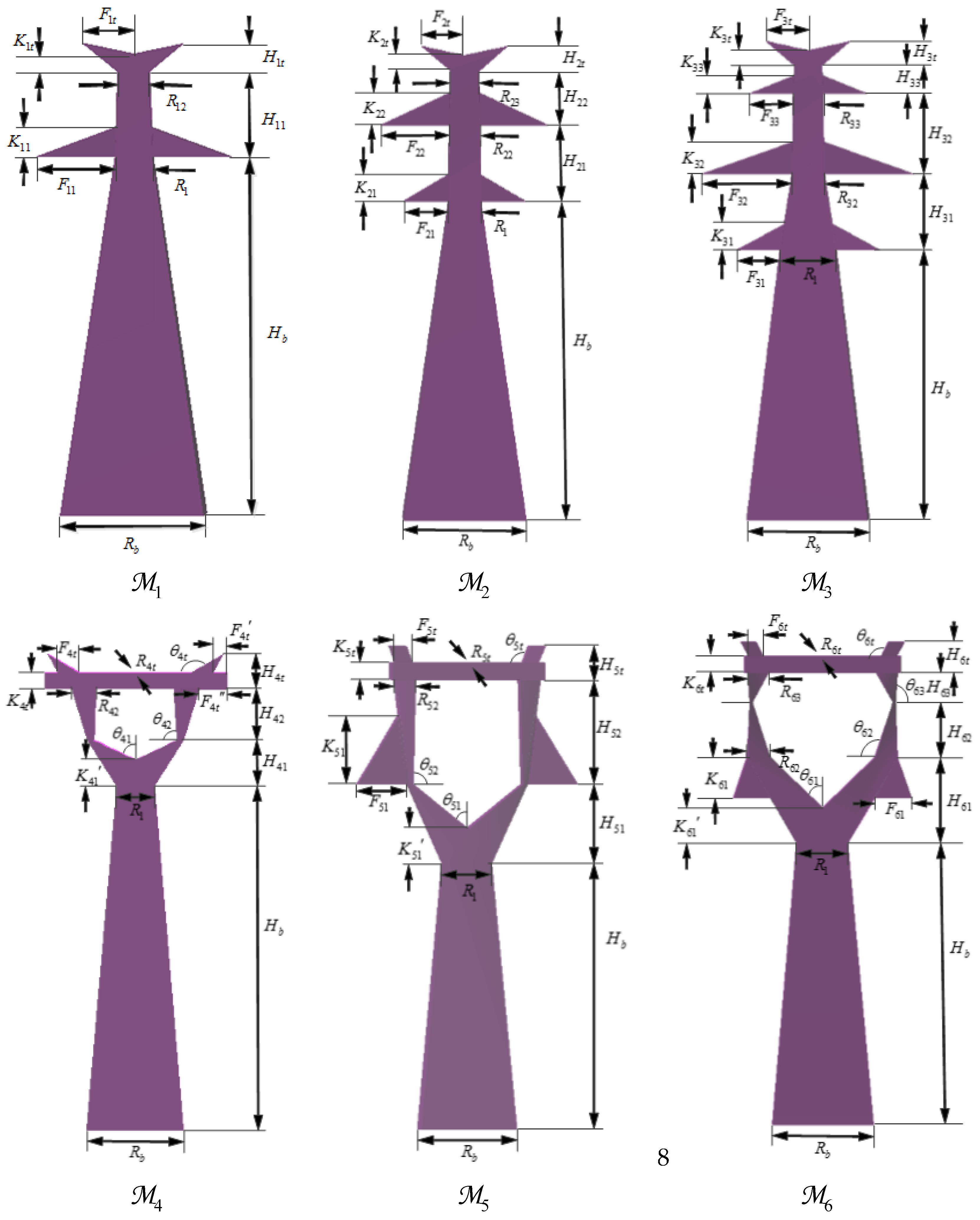
For simplicity, the pylon models are represented using polyhedrons. The parameters of the pylon models are shown in Figure 1. The pylon parameters are specified as the height, width of arms, the positions of turning points, and other specific parameters ($p_s$). Additionally, each pylon has general parameters ($p_g$): center point coordinates and main direction. Each pylon object reconstructed with this library is defined by an associated parameter set $\theta =\left(p_g,p_s\right)$.

The library includes a limited number of types. If a pylon cannot be reconstructed using a model in the library, a minimum external cube outside the data is used to represent the pylon object.

3.2. The Data-Driven Rough Type and Parameter Calculation

If we know the rough types and parameters of pylons, we can use a data-driven method [29] to effectively reconstruct the pylons. We design an effective kernel (jumping kernel $Q_2$ (Section 3.4.2)) to cleverly explore the optimal configuration and speedup the convergence by using the rough type and parameters.

Two general parameters of a pylon are first calculated. The center point XY coordinates are calculated using average values of the XY coordinates of all the points of the pylon. The center point Z coordinate is that of the lowest point of the pylon. The direction of the pylon can be calculated by analyzing the power lines connected to it. The rough direction of the pylon is set to be perpendicular to the power lines.

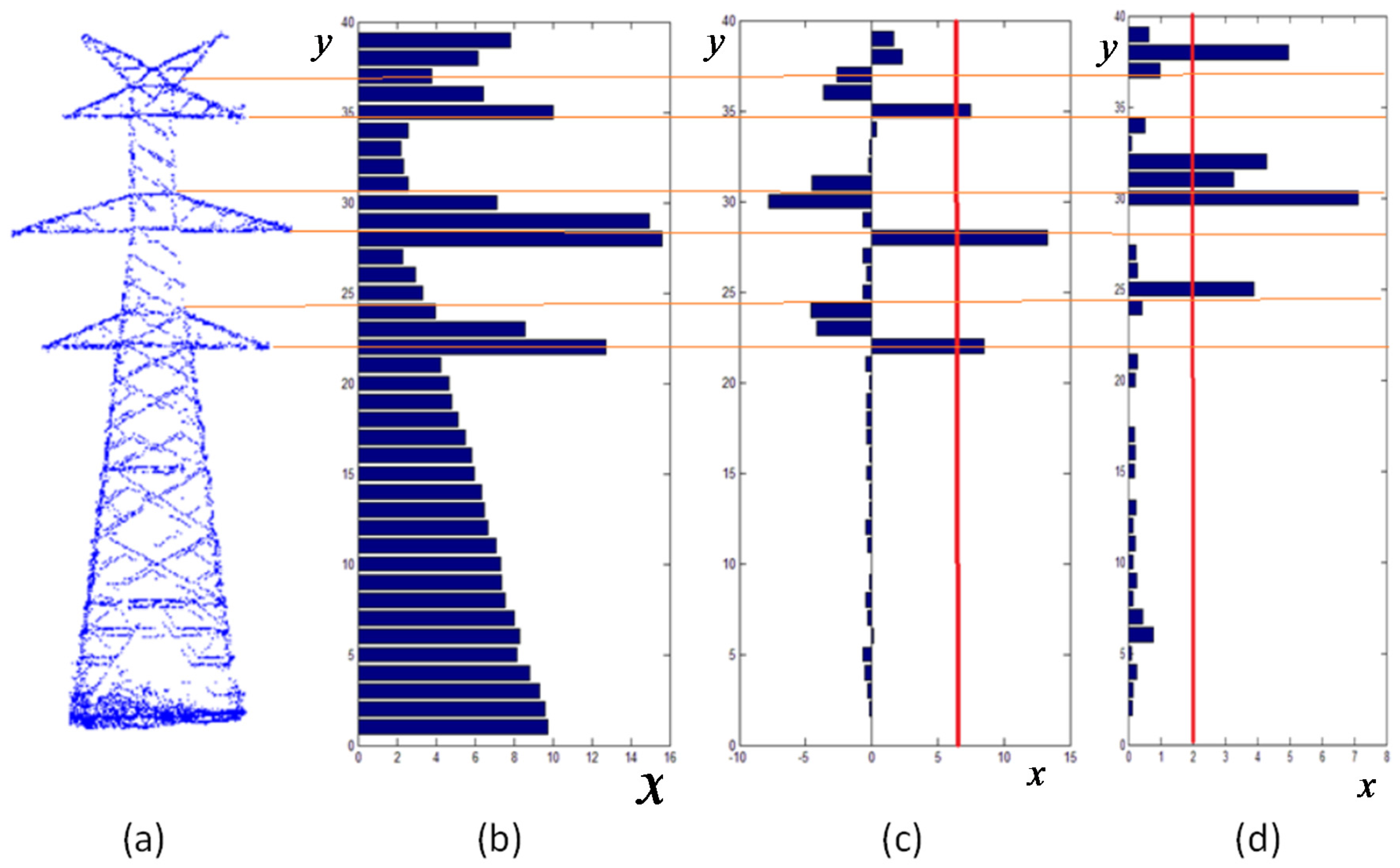
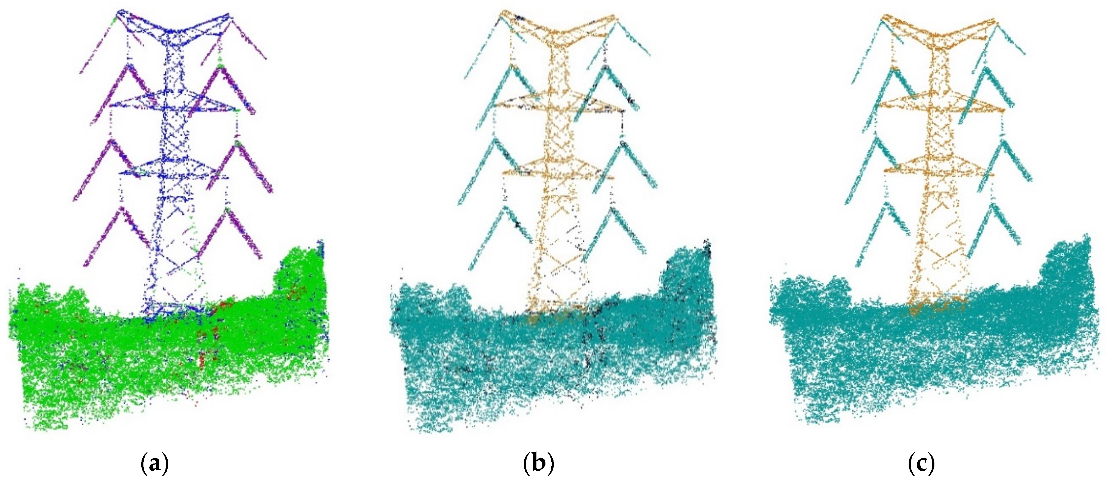
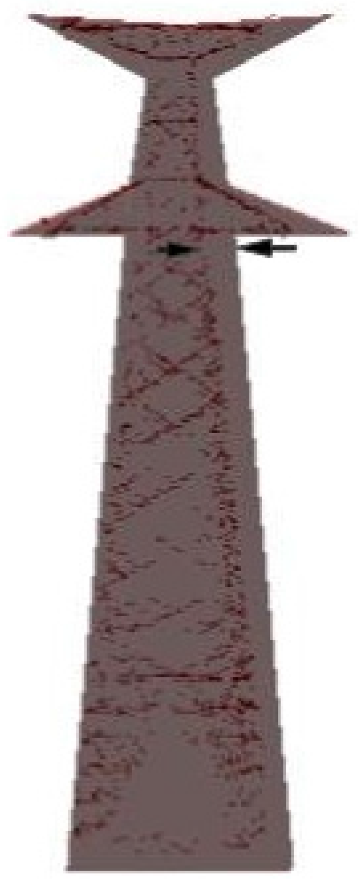
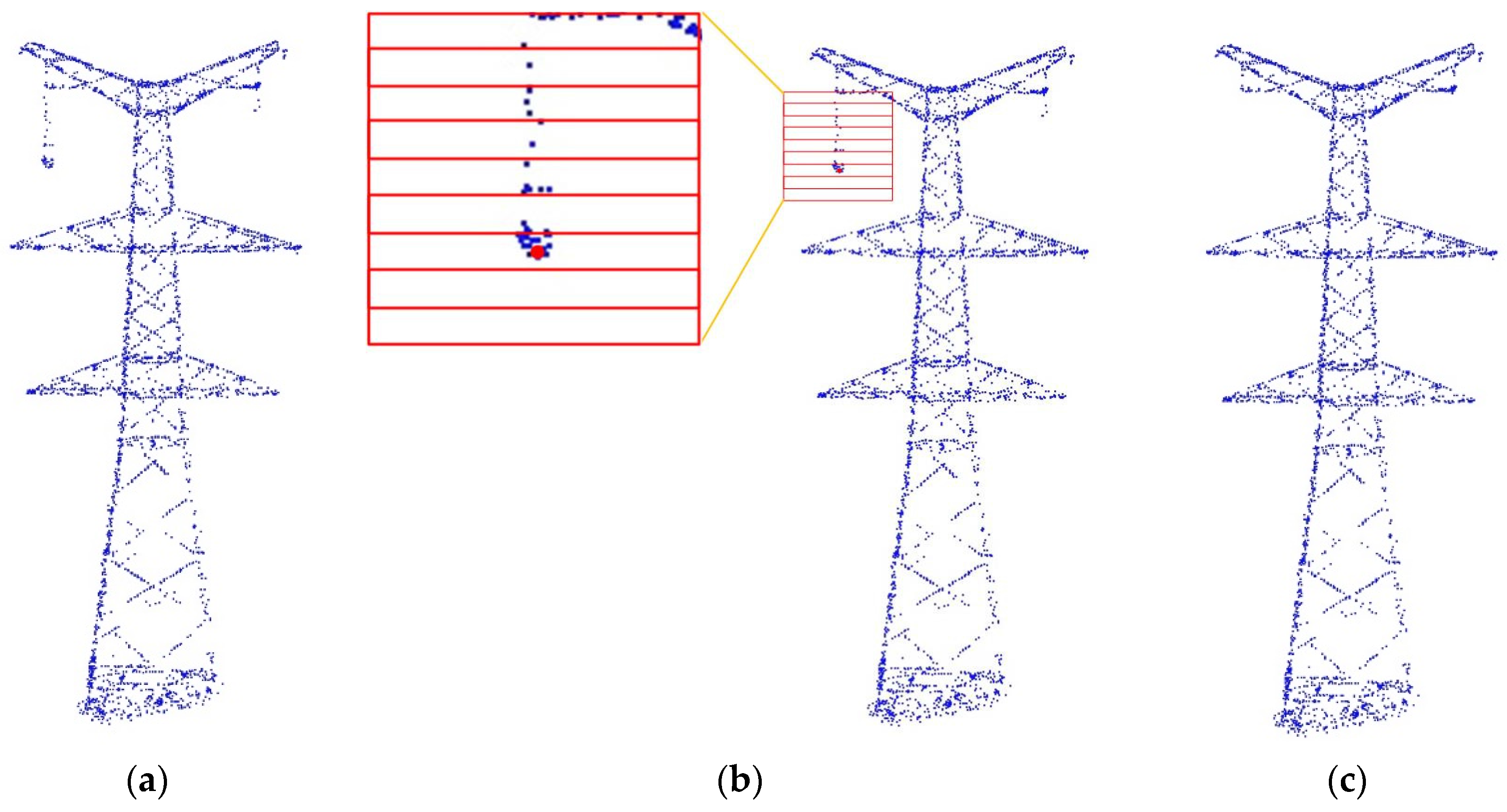
As seen in Section 3.1, the structures of pylons are regular, such as the cable arms being longer than their nearby parts. In order to determine the rough type and parameters of each pylon, we project all the points of a pylon onto its main plane (Figure 2a). A vertical profile is sliced into several bins of a certain distance. The histogram for the length of the sliced profile is shown in Figure 2b. The location of the arms can be determined by analyzing the changing length of the profiles. Usually, the projecting cable arms are longer than their nearby parts. The changing length of the arms can be represented using a derivative (Figure 2c). The pylon’s turning points, which represent the connecting locations of different parts, can be detected using a second derivative (Figure 2d). After determining the number and distribution of a pylon’s arms and turning points, we determine the rough type and parameters of this pylon by comparing it with models in the library.

3.3. Density and Gibbs Energy

In this section, we transform the reconstruction process (find the optimal types and parameters of pylons) to be a density optimization. The density is defined to measure the probability of the reconstructed objects corresponding to data of pylon points. The density can be defined in two ways: in a Bayesian framework, or through Gibbs energy. Using a Bayesian framework, the optimization is carried out over a posteriori density, which is obtained by multiplying the likelihood that provides the correspondence between the data and a configuration, by the a priori density. It needs complex computation of the normalizing constant. In this paper, a MCMC sampler coupled with a simulated annealing is used to the maximum density estimator $\widehat{x}=\arg \max h(\cdot )$. This estimator also corresponds to the configuration minimizing the Gibbs energy $U(\cdot )$, i.e., $\widehat{x}=\arg \min U(\cdot )$. This optimization technique is particularly interesting since the density does not need to be normalized (Equation (13)), and the complex computation of the normalizing constant is thus avoided [30].

The notation for the density and Gibbs energy is firstly listed:

$C$, the configuration space which represents the parameters of pylon objects.

$\mathcal{D}=\left({\mathcal{D}}_i\right)$, the data set of extracted pylon points, where ${\mathcal{D}}_i$ is a set of points of the $i$-th pylon.

$N$ is the number of pylons in the dataset.

$x$, an element of the configuration space $C$, which corresponds to a configuration of the 3D parametric model of the pylon. $x={\left(x_i\right)}_{i\le N}={\left(m_i,{\theta }_i\right)}_{i\le N}$, where each object $x_i$ is specified by both a model ${\mathcal{M}}_i$ of the library and an associated set of parameters ${\theta }_i$.

$d_m$, the number of parameters describing the model $m$.

In this section, a mapping from the probability space to the configuration is built. Reconstructing the objects consists of finding the configuration of objects $\widehat{x}$ by maximizing the density $\widehat{x}=\arg \max h(.)$.

The density under its Gibbs form:

$$h(x)=\frac{\exp -U(x)}{Z}$$

(1)

where $Z={\displaystyle {\int }_{X_t\in \mathsf{\Omega }}\exp \left(-U\left(x\right)\right)}$ is a normalizing constant. Moreover, the energy $U(.)$ can be expressed as a weighted sum of two terms: the data attachment term (Section 3.3.1) measures the consistency of the object configuration with respect to the measured points, and the regularization term (Section 3.3.2) favors or penalizes certain pylon configurations based on prior knowledge:

$$U(x)=U_d(x)+\beta U_p(x)$$

(2)

$\beta \in {\mathrm{R}}^{+}$ is a weighting parameter which tunes the importance of the prior energy versus the data energy.

3.3.1. Data Coherence Term

We now focus on the data coherence term $U_d\left(x\right)$, which aims at measuring the adequacy of reconstructed objects with respect to the extracted laser points of the pylons. The simplest way of defining it is to expand it as a sum over all objects in a configuration:

$$U_d\left(x\right)={\displaystyle \sum _{x_i\in X_t}{u}_d\left(x_i\right)}$$

(3)

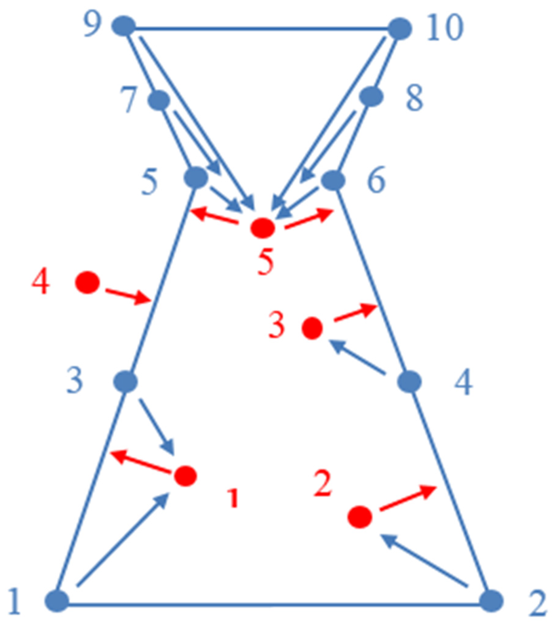
We now explain how the data term $u_d\left(x_i\right)$, mapping from a reconstructed object $x_i$ to be a real number, quantifies the relevance of an object with respect to its corresponding laser points. We naturally calculate the distance and measure the difference. The shorter the distance, the more likely the probability of finding a good object. The shapes of the pylon model represented using non-convex polyhedrons with multi-faces are complex. A shape may cause deviation if only the distances from the laser points to an object are used. As shown in Figure 3, the part of the object that is higher than red point 5 is a vacancy without any laser points. However, the closest distance from red point 5 to the object cannot touch that part. Therefore, we design the distance with two mutual parts: (1) a normalized distance from the point set ${\mathcal{D}}_i$ to object $x_i$ (denoted by red arrows in Figure 3); and (2) a normalized Hausdorff distance from the key point set (corner points and central points of faces) of object $x_i$ to the measured point set ${\mathcal{D}}_i$ (denoted by blue arrows in Figure 3).

(1) Normalized Distance from Point Set ${\mathcal{D}}_i$ to Object $x_i$

We consider that a good object model should contain as many as laser points and the distance from laser point to the object model should be as near as possible. In order to penalize the points outside of the object, the distances of the points in and out of the object should have different weights. Because the models are represented using polyhedrons, whether a point in or out of a model (polyhedron) can be determined referring to the work of Schneider and Eberly [31].

We first define a normalized distance $D_n$ from a laser point $s$ to its corresponding object $x_i$, where the value of a point outside the object is bigger than that of a point inside the object:

(a) If point $s$ is in the object $x_i$:

$$D_n\left(x_i,s\right)={\delta }_i\frac{D}{D_{\max }}$$

(4)

(b) If point $s$ is out the object $x_i$:

$$D_n\left(x_i,s\right)={\delta }_o\frac{D}{D_{\max }}+{\delta }_i$$

(5)

where $D$ is the nearest Euclidean distance from point $s$ to object $x_i$, which can be calculated by referring to the work of Schneider and Eberly [31]. $D_{\max }$ is the largest value of $D$. ${\delta }_i$ and ${\delta }_o$ are two parameters that restrict the value of the normalized distance to a certain range. We set ${\delta }_i+{\delta }_o=1$ and ${\delta }_i=0.2$.

After defining the normalized distance of a single point, the total normalized distance from the point set ${\mathcal{D}}_i$ to object $x_i$ is set to be:

$$\Gamma \left({\mathcal{D}}_i\to x_i\right)=\frac{1}{N}{\displaystyle \sum _{s\in {\mathcal{D}}_i}{D}_n\left(x_i,s\right)}+\max \left(D_n\left(x_i,s\right)\right)$$

(6)

where $s\in {\mathcal{D}}_i$ is every point in the point set, N is the number of points.

$\Gamma \left({\mathcal{D}}_i\to x_i\right)$ has two parts: a mean and a maximum of the normalized distance. The mean value term is used to avoid the effects of different data densities. The maximum distance term is used to avoid the situation of partial mismatch.

(2) Normalized Hausdorff distance from the key point set of object $x_i$ to the measured point set ${\mathcal{D}}_i$

The Hausdorff distance from the key point set ${\mathcal{K}}_i$ of object $x_i$ to the measured point set ${\mathcal{D}}_i$ is:

$$h\left({\mathcal{K}}_i,{\mathcal{D}}_i\right)=\underset{a\in {\mathcal{K}}_i}{\max }\left\{\underset{b\in {\mathcal{D}}_i}{\min }\left\{d\left(a,b\right)\right\}\right\}$$

(7)

where $d\left(a,b\right)$ is the Euclidean distance of points a and b. In order to calculating the Hausdorff distance, we first calculate the nearest distance from the key point a of object to its nearest laser point b (denoted by blue arrows in Figure 3). Then, the largest distance of the key point to be the Hausdorff distance from the key point set ${\mathcal{K}}_i$ of object $x_i$ to the measured point set ${\mathcal{D}}_i$.

The normalized Hausdorff distance is then set to be:

$$\Gamma \left(x_i\to {\mathcal{D}}_i\right)=\frac{h\left({\mathcal{K}}_i,{\mathcal{D}}_i\right)}{H_{\max }}$$

(8)

where $H_{\max }$ is the largest value of $H$.

Finally, the data term $u_d\left(x_i\right)$ defined using the distance is:

$$u_d\left(x_i\right)=\Gamma \left({\mathcal{D}}_i\to x_i\right)+\Gamma \left(x_i\to {\mathcal{D}}_i\right)$$

(9)

3.3.2. Regularization Term

The regularization energy $U_p(x)$ is used to favor certain configurations of objects and to penalize certain others. It introduces interactions between neighboring objects. This reduces to the definition of a combination of simplified energy terms $U\left(v,w\right)$, where $v$ and $w$ are different objects. A neighborhood relationship must be set up to define the interactions: two distinct objects $x_i$ and $x_j$ are said to be neighbors if they are connected by power lines. The neighborhood relationship is denoted by $\sim$($i\sim j$ represents the set of neighboring pairs).

The regularization term is expressed through summing all the two neighboring objects $x_i$ and $x_j$:

$$U_p\left(x\right)={\displaystyle \sum _{i\ne j}{1}_{\left\{x_i\sim x_j\right\}}}g\left(x_i,x_j\right)$$

(10)

where $1(.)$ is the characteristic function. The function $g(.)$ is defined as a mapping from ${\mathrm{R}}^{d_{m_i}}\times {\mathrm{R}}^{d_{m_j}}$ to $[-1,0]$ based on neighboring objects $x_i$ and $x_j$.

In order to avoid electric shock, the power lines between neighboring pylons should be parallel and have sufficient gaps. In this way, the construction of neighboring pylons will satisfy certain demands. The function $g(.)$ is defined in two situations:

(1) If the types of objects $x_i$ and $x_j$ are the same, the parameters are encouraged to be same in order to keep the power lines parallel:

$$g\left(x_i,x_j\right)=\frac{1}{K}{\displaystyle \sum _k\frac{D_k\left(x_i,x_j\right)}{D_k^{\text{max}}}}-1=\frac{1}{K}{\displaystyle \sum _k\frac{\left|{\tilde{\theta }}_i^k-{\tilde{\theta }}_j^k\right|}{D_k^{\text{max}}}}-1$$

(11)

where, $K$ is the number of the parameters, ${\tilde{\theta }}_i^k$ and ${\tilde{\theta }}_j^k$ are the k-th element of the parameter sets of objects $x_i$ and $x_j$, respectively. We set D_k to be the k-th parameter distance and $D_k^{\text{max}}=\max D_k\left(x_i,x_j\right)$ is the maximum value of the k-th parameter distance. In this term, the closer the parameters of the two objects, the lower the energy.

(2) If the types of objects are different, the neighboring objects should be compatible to carry the same power lines. The compatibility of pylons is defined in Section 3.1. In this way, we simply define the function $g(.)$ to be a certain value:

$$g\left(x_i,x_j\right)=g_c$$

(12)

Since different types of pylons connected by power lines are used much less than the situation of the same type, we set $g_c$ to be the maximum value of situation 1 (same pylon type), which can be learned by analyzing a training set. It is also easy to re-learn when changing the kind of data used.

Otherwise, the energy will be null.

3.4. Optimization

We now find the object configuration by maximizing the density $h(.)$. This is a non-convex optimization problem in a high and variable dimension space $C$, since the models of pylons in the library $\mathcal{M}$ are defined by different numbers of parameters. To sample from $h(.)$ (i.e., to obtain some configurations of objects), a solution is to use an MCMC method. Such a procedure builds a Markov chain ${\left(X_t\right)}_{t\ge 0}$ on the space of finite configurations of objects using a starting point $X_0$ and a Markovian transition kernel $Q\left(x,.\right)$, which converges toward the target distribution (specified by the density $h(.)$).

There are two basic requirements for Markov chain design [29]. Firstly, the Markov chain should be ergodic. That is, from an arbitrary initial statement of configuration $X_0$, the Markov chain can visit any other states $x\in C$ in finite time, and converge to the required invariant distribution. In order to ensure the ergodicity, the jumping and non-jumping transformations (Section 3.4.2) introduced converge to the desired distribution in this paper. Secondly, the Markov chain should have a stationary probability. This is replaced by a stronger condition of detailed balance equations which demand that every move should be reversible. The Metropolis-Hastings-Green MCMC framework [32,33,34] used in this paper satisfies the detailed balance and reversibility requirements.

3.4.1. MCMC Procedure

The classical MCMC methods for constructing suitable transition kernels are well known. The two most popular methods are the Gibbs sampler [35] and the Metropolis-Hastings method [33,34]. However, these methods cannot handle dimension jumps, i.e., changes in dimension between samples. The reversible jump MCMC algorithm based on Metropolis-Hastings samplers in the general state spaces [32] allows us to deal with a variable dimension state space. This technique has shown potential in various applications such as image segmentation [29] and architectural object reconstruction [19,36].

The Metropolis-Hastings-Green sampler simulates a discrete Markov chain ${\left(X_t\right)}_{t\ge 0}$ on the configuration space, which converges toward an invariant distribution (specified by the density, $h(.)$). The transitions of this chain correspond to perturbations of the current configuration $x$. We use the transitions of this chain corresponding to local perturbations, which means that only the parameters of one pylon object of the configuration is generally concerned with a perturbation of the current configuration. Each iteration of the sampler is composed of two steps. The first step consists of proposing a new state $y$ by perturbing the current state $x$ by using proposition kernels $Q_m\left(x,\cdot \right)$. The second step decides whether the perturbation is accepted to define the new state $y$.

The acceptance ratio of a proposition from $x\to y$ is given by:

$$R_m\left(x,y\right)=\frac{\pi \left(dy\right)Q_m\left(\mathrm{y},dx\right)}{\pi \left(dx\right)Q_m\left(x,dy\right)}$$

(13)

where $\pi (.)$ is the target distribution defined on configuration space $C$ and specified by the density $h(.)$, as defined in Section 3.3; and $Q_m\left(.,.\right)$ is the proposition kernel, which allows us to propose the different types of perturbations specified in Section 3.4.2.

The acceptance probability of a perturbation from $x\to y$ is then expressed by: $\alpha =\min \left(1,R\left(x,y\right)\right)$.

In summary, the MCMC sampler is:

• Input: An initial configuration $X_0$
• Repeat

  • Choose a proposition kernel $Q_m$ with probability $q_m$
  • Build a new configuration $X_{new}=y$ from $X_t=x$ w.r.t. the selected kernel
  • Compute the acceptance ratio $R_k\left(x,y\right)$
  • Compute the acceptance rate $\alpha =\min \left(1,R_k\left(x,y\right)\right)$
  • Take $X_{t+1}=y$ with probability $\alpha$ and reject it otherwise.
• Until convergence

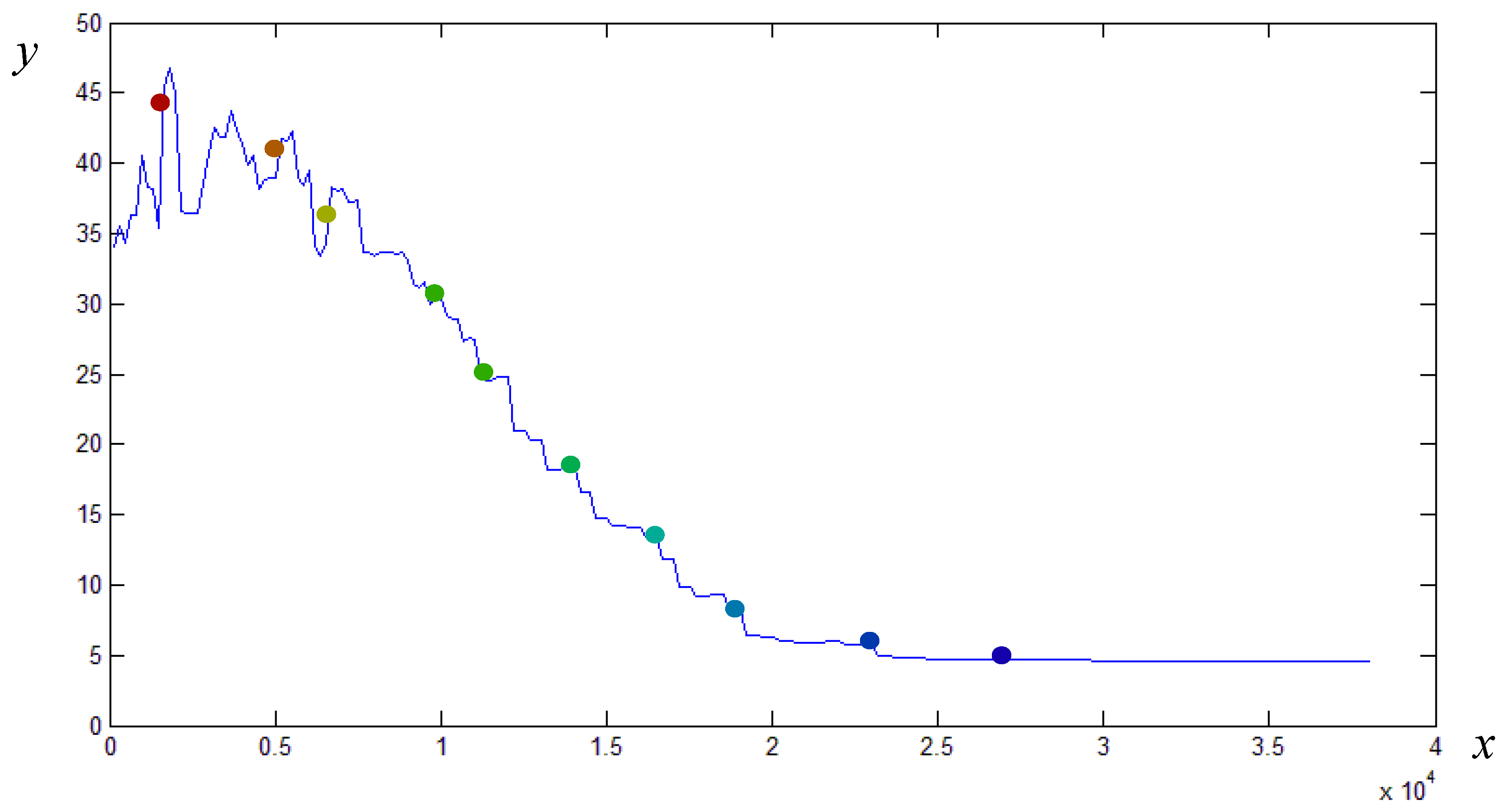
An MCMC algorithm has converged if its output can be safely thought of as coming from the true stationary distribution of the Markov chain. The convergence can be monitored through many methods, such as: Monte Carlo error checking [37,38] and the Celman-Rubin method [39]. We mainly analyze the convergence through checking the trance plot. When the trance plot is stable, and without obvious trend and periodicity, the MCMC algorithm are thought to be converged.

3.4.2. Proposition Kernels

The kernels are designed in order to make the Markov chain converge to the desired distribution. The kernel specification plays a crucial role in the efficiency of the sampler. By proposing object configurations of interest, these appropriate kernels allow acceleration of the convergence by avoiding rejection of too many candidates.

We introduce two kinds of kernels in this paper: (1) jumping transformations; and (2) non-jumping transformations. The jumping kernels mainly explore the transformation direction of the configuration, and favor configurations that have a high density. The non-jumping kernels contribute to a detailed adjustment of the object parameters when the configuration is close to the optimal solution.

A kernel performs a perturbation from an object $x_i$ to an object ${\widehat{x}}_i$, such that the current object configuration $x={\left(x_p\right)}_{p\in C}$ is perturbed into the configuration $y={\left(x_p\right)}_{p\in C-\left\{i\right\}}\cup {\widehat{x}}_i$.

(1) Jumping transformations 

Let us consider a perturbation from an object $x_i$ of type ${\mathcal{M}}_m$ to an object ${\widehat{x}}_i$ of type ${\mathcal{M}}_n$. A bijection [32] between the parameter space of the object types ${\mathcal{M}}_m$ and ${\mathcal{M}}_n$ is created: $x_i$ is completed by auxiliary variables $u_{mn}$ simulated under a law ${\phi }_{mn}(.)$ to provide $\left(x_i,u_{mn}\right)$, and ${\widehat{x}}_i$ by $v_{nm}\sim {\phi }_{nm}(.)$ into $\left({\widehat{x}}_i,v_{mn}\right)$, such that the mapping ${\mathsf{\Psi }}_{mn}$ between $\left(x_i,u_{mn}\right)$ and $\left({\widehat{x}}_i,v_{mn}\right)$ is a bijection:

$$\left({\widehat{x}}_i,v_{mn}\right)={\mathsf{\Psi }}_{mn}\left(x_i,u_{mn}\right)$$

(14)

The ratio of the kernels in the acceptance ratio (Equation (13)) is then expressed by:

$$\frac{Q_k\left(\mathrm{y},dx\right)}{Q_k\left(x,dy\right)}=\frac{J_{nm}^{\left(k\right)}{\phi }_{nm}^{\left(k\right)}\left(v_{nm}\right)}{J_{mn}^{\left(k\right)}{\phi }_{mn}^{\left(k\right)}\left(v_{mn}\right)}\left|\frac{\partial {\mathsf{\Psi }}_{mn}\left(x_i,u_{mn}\right)}{\partial \left(x_i,u_{mn}\right)}\right|$$

(15)

where $J_{mn}$ corresponds to the probability of choosing a jump from ${\mathcal{M}}_m$ to ${\mathcal{M}}_n$. The following jumping transformation kernels, i.e., distributions $\left(J_{mn},{\phi }_{mn}\right)$, are used in this paper:

Kernel $Q_1$. This kernel proposes a new state according to a uniform distribution that ensures the Markov chain can visit any configuration of the state space:

$$J_{mn}^1=\frac{1}{card\left(\mathcal{M}\right)}$$

(16)

$${\phi }_{mn}^1=u_{K_{mn}}$$

(17)

where $u_{K_{mn}}$ is a distribution which distributes uniformly on domain $K_{mn}$ of parameter $u_{mn}$.

This kernel is classic. The use of this single kernel is inefficient and thus we propose additional efficient kernels that explore the optimal configuration.

Kernel $Q_2$. In Section 3.2, we described how the rough types and parameters of the pylons are determined. This information can be used to accelerate the convergence speed. This kernel cleverly explores the state space using a data-driven process and is efficient [29]. The state $x$ is proposed knowing the data. The probabilities $J_{mn}^2$ are focused on models of rough types. The state parameter $x_i$ of pylon object $i$ is proposed knowing the rough parameters ${\tilde{x}}_i$ according to the Gaussian distribution $\mathcal{N}\left({\tilde{x}}_i,{\delta }_2{\mathbf{I}}_{d_i}\right)$; in practice, we set $\delta =1$ m.

Kernel $Q_3$. In power engineering, the adjacent pylons are commonly built with the same structures in order to be well-regularized and keep the power lines parallel. Thus, the types and parameters are the same. In this kernel, the parameter values of object $x_i$ are chosen depending on its neighboring objects. The probabilities $J_{mn}^3$ are focused on some models of neighboring objects whose types are the same as object $x_i$. The state parameter of object $i$ is proposed knowing the neighboring object ${\tilde{x}}_j$ according to a Gaussian distribution $\mathcal{N}\left({\tilde{x}}_j,{\delta }^2{\mathbf{I}}_{d_j}\right)$. Although this kernel is very useful for optimizing the configuration statement, it can block the current configuration in a local optimum. Thus, this kernel is used when the current configuration is close to the optimum.

(2) Non-jumping transformations 

Non-jumping transformations do not involve changing the dimension of the configuration. Such a transformation randomly selects one object $x_i$ in the current configuration and perturbs it to obtain a new version ${\widehat{x}}_i$. Instead of using uniformly generated parameters (kernel $Q_1$), the perturbation is a zero-mean Gaussian random variable with variance ${\delta }^2{\mathbf{I}}_{d_i}$:

$${\widehat{x}}_i|x_i\sim \mathcal{N}\left(x_i,{\delta }^2{\mathbf{I}}_{d_i}\right)$$

(18)

A Gaussian perturbation can be used to adjust details of the parameters rather than greatly changing their values.

A random walk is introduced to perform a local exploration of the configuration. The suitable acceptance ratio R (Equation (13)) is simply given by:

$$R\left(x,y\right)=\frac{h\left(x\right)}{h\left(y\right)}$$

(19)

We set the process into two stages. At the beginning, when the accepted proposition rate is high, the process explores the density modes and favors configurations which have a high density. In this exploration stage, the jumping kernels are mainly used ($\frac{1}{4}{q}_j=q_{nj}=0.2$). When the accepted proposition rate computed on 1000 iterations becomes lower than 0.05, the configuration is close to the optimal solution and does not evolve very much: it involves a detailed adjustment of the pylon parameters. In this second stage, the non-jumping kernel is mainly used ($q_j=\frac{1}{4}{q}_{nj}=0.2$). In each stage, the jumping kernels are used equally ($q_1=q_2=q_3=\frac{1}{3}$).

3.4.3. Convergence Associated Using Simulated Annealing

Simulated annealing is used to ensure convergence [34]. The MCMC sampler is coupled with simulated annealing in order to find the optimum of the density. Instead of $h(.)$, we use $h{(.)}^{\frac{1}{T_t}}$ in the optimization process, where $T_t$ is a sequence of decreasing temperatures that tend to zero as $t$ tends to infinity. Simulated annealing theoretically ensures convergence to the global optimum for any initial configuration $X_0$ using a logarithmic temperature decrease; however, it is slow. In order to speed up the processing, we use a geometric decrease which gives an approximate solution close to the optimal one. Such a decrease was detailed in [40]. The initial and final temperatures are estimated by sampling the configuration space and considering the variance of the global energy [41].

4. Test Area and Data Characteristic

Our results show the reconstruction of complex pylons in a test area. The terrain is complex, with undulating and discontinuous characteristics. The vegetation is dense and tall. Tall trees could be wrongly classified to be pylons due to the high point density and big height difference. In order to analyze the effectiveness of our methods, we selected an area with a length greater than 20 km along, which contains more than 100 pylons. In order to be clear, we shown typical reconstruction results of two regions in Section 5, and the results of other pylons are similar.

The results were obtained using a dataset for power line management, acquired from Yi Chang, Hubei, China. The data were collected using a Riegl Q560 laser measurement system. The parameters of the flight and the settings of the sensor are shown in

Table 1. Data characteristic.

	Flying Height	Flying Speed	Scan Angle	Rate
Data	200–600 m	30 km/h	22.5°	200 kHz

. Due to the topography, the flying altitude varied significantly. We first extracted the pylons from the point cloud data, and then the pylons were reconstructed using the methods introduced in this paper.

5. Experimental Analysis

5.1. Pylon Extraction

The accuracy of the pylon point extraction is of importance for the reconstruction. We first automatically classify a dataset into different classes. The outliers are then eliminated using graph cut and contextual information.

5.1.1. Point Cloud Classification

As mentioned previously in Section 2.1, we use a JointBoost classifier for the point cloud data classification. In the training step, object-based balanced sampling is important. In our study, the training step was performed with 4000 samples (points with true labels) per class, except pylons, randomly selected from the training dataset. The number of training samples for the pylons were selected to be 8000, twice the number of each other class in order to improve the pylon extraction accuracy. Another part of the training set was randomly chosen as a validation set. The validation set was used to measure the effectiveness of the classifier parameters. The trained classifier was then used to classify the test data.

A finely trained JointBoost classifier with well-selected features can generate good classification results [7]. Testing data were manually labeled as classes of ground truth for calculating the classification accuracy. The classification precision and recall are shown in

Table 2. Classification accuracy.

Overall Accuracy: 94.9%
--	Ground	Vegetation	Building	Power-line	Pylon
Precision	95.8%	92.1%	91.3%	89.6%	93.5%
Recall	97.8%	87.7%	89.1%	86.4%	78.2%

.

A typical automatic pylon extraction result using the JointBoost classifier is shown in Figure 4a.

Although the precision of the automatic classification is high, the pylon recall is low. There are also many local errors in the pylon classification results (see Figure 4a). Misclassified points are first found in pylons where they are labeled as power lines. The main reason for this is that the structure of a pylon consists of multiple metallic triangles for stabilization, and the sides of the triangles share the same linear structure characteristics as power lines. There are also many false vegetation points that belong to pylons. This is because the densities of pylon points vary in different regions, especially the intersection regions between power lines and pylons, and regions near the ground. This misclassification will badly affect the pylon modeling results. Therefore, before reconstruction, the outliers of the pylon classification need to be eliminated.

5.1.2. Outlier Elimination

The initial pylon classification results have certain features: (1) major parts of the pylons are correctly classified; and (2) local errors are randomly distributed and are few in number. Because pylons are usually separated from other objects, we first use graph cut [28] to eliminate the local errors on the pylons. The two graph-cut key points include foreground/background seed point selection and graph building.

The initial classification results produced by JointBoost are used to generate the foreground/background seed constraints. A region growing algorithm is first used to cluster nearby points with the same initial classification labels. We consider objects with a large number of cluster points to be reliable, while objects with a small number of cluster points are considered to be unreliable. The thresholds for reliable objects of the different kinds are obtained using the training dataset. For pylon extraction, the points of a reliable pylon are selected to be the foreground seed points. The points of other reliable objects close to the reliable pylon are selected to be the background seed points.

A graph representing the structure of the point cloud is created before segmentation. In this graph, the edges are constructed with a k-nearest system for the input points. The closer points are more strongly connected than the other points.

Segmenting the object of interest from its background is formulated as a binary labeling problem. Boykov and Funka-Lea demonstrated how to construct a binary energy function using a graph cut and foreground/background seed constraints [28]. They then showed how this energy function can be optimized with a min-cut algorithm.

Figure 4 shows the foreground/background segmentation for a pylon neighborhood. Figure 4a shows the initial classification using the JointBoost classifier and local features, where it can be seen that there are many error points in the pylon. Figure 4b shows the foreground and background seed points. As for segmentation, points in the reliable pylon are treated as the foreground seed points, while points in other reliable objects (power lines, vegetation) are treated as the background seed points. Figure 4c shows the segmentation results, where it can be seen that the segmentation results are smooth.

After graph-cut processing, in the intersection regions between power lines and pylons, many non-pylon points are still misclassified as pylons (Figure 5a). These misclassified points have a lower density than other parts of the pylons. In order to detect this kind of corresponding misclassified point of a pylon, we first project the pylon points onto its main plane and detect the intersection points of the power lines with this plane. The neighboring points of a power line are then sliced into several bins of a certain distance (Figure 5b). The width of the bin is selected based on that of the arms. The bins with fewer points are considered to be non-pylon.

5.2. Pylon Reconstruction

5.2.1. Reconstruction Evolution

As described above, the reconstruction process simultaneously determine the type and fit its parameters of a pylon. The evolution of the reconstruction at different steps of the algorithm on some sample pylons is first illustrated in Figure 6.

At the beginning of the process, when the temperature is high, the process mainly explores the types. There are, however, many objects that are not well identified and reconstructed. The jump plays an important role by specifying the types of objects. Then, as long as the temperature decreases, more and more objects are well reconstructed, and some objects begin to find their rough configuration. At a low temperature, the non-jumping perturbation is useful at this stage mainly to perform a detailed adjustment of the object parameters. Finally, all the objects are well reconstructed, until convergence. The associated energy decrease graph is presented in Figure 7.

5.2.2. Results of Reconstruction

We selected two typical regions to demonstrate the reconstruction results (Figure 8 and Figure 9). The results of other pylons are similar. The models are shown as semi-transparent in order to evaluate the reconstruction quality by checking the accordance of the reconstructed models and the laser points. Overall, the results are convincing. The reconstructed pylon models are attached to the points of the pylons very well. Even if some details are mismatched with the data, the shapes of the objects compare well to the ground truth. In the reconstruction process, the data coherence term mainly contributes to the shape reconstruction. When there is data loss, the regularization term provides helpful information concerning the models of the neighboring pylons.

The reconstructed main parts of pylons are good and coherent to the extracted laser points. Some tiny reconstruction errors are mainly caused by the reconstruction methods. In parts with few points, the details of reconstruction are not precise. It is because that pylon parts with few points contribute little to the data coherence term in the energy calculation. The MCMC sampler usually cannot find an absolute optimization.

6. Discussion

We introduced a method for pylon reconstruction in this paper. The quantification and errors of reconstruction are mainly discussed in this section.

6.1. Reconstruction Quantification

As seen in Section 5.2, because the pylons in the test areas can be well represented using the models in the library (Section 3.1), all the types of reconstructed pylons have been correctly identified. Thus, there are no gross errors.

The errors are mainly due to the mismatch of laser points to the reconstructed pylon models. In order to quantify the reconstruction results, we mainly checked the distance between the reconstructed models and the laser points

Two indicators were introduced for the quantitative evaluation:

(1) Root-mean-square error (RMSE)

RMSE represents the sample standard deviation of the difference between predicted values and true values. We used the RMSE to evaluate the difference between the laser points and reconstructed object models in the dataset. In the EMSE calculating, the difference measured by using the closest distance of a laser point to its corresponding model. We calculated all the extracted pylon points in the test area, other than analyzing one pylon by one.

The RMSE is defined to be:

$$\delta =\sqrt{\frac{{\displaystyle {\sum }_{i=1}^{N_t}{\displaystyle {\sum }_{j=1}^{N_i^m}{\left(d_j^m\right)}^2}}}{{\displaystyle {\sum }_{i=1}^{N_t}{N}_i^m}}}$$

(20)

where $N_t$ is the tower number in the dataset, $N_i^m$ is the measured point number of the i-th tower, and $d_j^m$ is the closest distance of the j-th point to its corresponding object model.

The RMSE for the pylon reconstruction in this study was 0.12 m, which is a promising result.

(2) Max distance

The mismatch can be represented using distance. We use the max distance to detect the extreme mismatch of laser points and the models.

We evaluated two kinds of distance: a max distance from laser points to object models, and a max Hausdorff distance from the key points of object models to laser points.

The max distance from the laser points to the models was 0.32 m, while that from key points of the models to laser points was 0.37 m. These values are three times bigger than the RMSE, which means that the mismatch is not uniformly distributed. The two max distances are almost the same because we used two mutual distances in the data coherence term.

The reasons of reconstruction mismatch are mainly discussed below.

6.2. Reconstruction Errors

Globally speaking, the different pylon types were correctly identified. Even if some details are omitted, the shapes of pylons compare well to the ground truth (see Section 5.2.2). The details mismatched to the data mainly occur in pylon parts with few points. There are two reasons for this.

(1) Pylon parts with few points contribute little to the data coherence term in the energy calculation. The data coherence energy term have been defined with mutual distances between the points and objects. The distance could be wrongly calculated due to the omitting of data.

A solution to this could be to introduce effective primitive knowledge about these parts to expand them using only distance in the data coherence term.

(2) The MCMC sampler usually cannot find an absolute optimization, but only an approximate global optimization in finite procedures in finite time. The pylon parts with few points, which contribute little to the energy calculation, thus cannot precisely reconstructed by searching the approximate global optimization.

Besides the mismatch error of reconstruction, an extreme situation that can cause the pylons to be poorly reconstructed is the abnormal movement of pylons. A normal pylon is usually vertical. If there is inclination and curvature, the model-based reconstruction methods cannot adapt to it. As shown in Figure 10, the gap between the measured points and reconstruction object is caused by the inclination. Thus, the reconstruction errors can be used to find the abnormal movement of pylons.

Pylons hold power lines, resisting the force of side wind. Therefore, the stability of the pylons is important for power safety. An unusual movement might damage the stability of a pylon. If there is an inclination or curvature, the pylon must be repaired.

In this Section, we have discussed the accuracy of reconstruction and reasons of errors above. Based on pylon points’ extraction and outliers’ elimination, the method can precisely reconstruct pylons with high accuracy. Because there were few works of pylon reconstruction, we have not compared our work with others. Due to the limitation of the library, this method is not suitable for reconstructing pylon types that are not defined in the library. If a pylon cannot be reconstructed using a model in the library, a minimum external cube outside the data is used to represent the pylon object. Then, the types of pylons in the library must be increased.

In different situations (such as different countries), the pylon types may vary greatly. Reconstruction failures might be caused by using a not suitable library. Therefore, the library must be updated to adapt the new situations. Because the pylons are usually constructed with specification and the models can be parameterized, the updating of library can be done conveniently. Based on the well-defined library, the pylon models are automatically reconstructed using an energy optimization method. The reconstruction method introduced in this paper thus is robust and effective.

7. Conclusions

We have presented a reliable algorithm to reconstruct pylons from airborne LiDAR data using stochastic geometry based on a model library. The method has several important characteristics and it provides very good results for pylon reconstruction from point cloud data. The advantages and efficiencies of the proposed algorithm are mainly based on two aspects. The first is the definition of the energy to be minimized; the second is the choices and efforts made in the implementation. Regarding the energy, we take into account both low-level information considering the data coherence degree of the laser points with the pylon objects, and geometric knowledge about the connected disposition of neighboring pylons. In the implementation, we use an MCMC sampler associated with well-designed kernels to optimize the energy, considering both precision and efficiency. Overall, the pylon reconstruction results are accurate and convincing.

In our future work, we will attempt to improve the reconstruction results. As it is, using only distance in the data coherence term of the energy can cause the reconstruction of some tiny parts with few points to be less precise. A primitive-combining energy optimization could improve the reconstruction of details for these parts with few points. It would also be interesting to introduce more efficient kernels. In fact, at the beginning of the process, when the temperature is high, most of the moves (jumping and non-jump) are accepted. As long as the process evolves, perturbations (mainly non-jump) become dominant. In the process, the kernels play a key role in the convergence. More efficient data-driven kernels should therefore be introduced.

The proposed method is an adaptive method since other models could be added to the library depending on the context. This method could also be adapted to higher-rank voltage power lines by extending the library according to future specifications. The methods introduced in this paper could also be used for other kinds of regular object reconstruction, such as street lamps and dustbins.

References

1. Katrasnik, J.; Pernus, F.; Likar, B. A survey of mobile robots for distribution power line inspection. IEEE Trans. Power Deliv. 2010, 25, 485–493. [Google Scholar] [CrossRef]
2. Aggarwal, R.K.; Johns, A.T.; Jayasinghe, J.A.S.B.; Su, W. An overview of the condition monitoring of overhead lines. Electric Power Syst. Res. 2000, 53, 15–22. [Google Scholar] [CrossRef]
3. Ahmad, J.; Malik, A.S.; Xia, L. Vegetation monitoring for high-voltage transmission line corridors using satellite stereo images. In Proceedings of the National Postgraduate Conference (NPC), Kuala Lumpur, Malaysia, 19–20 September 2011; pp. 1–5.
4. Ashidate, S.-I.; Murashima, S.; Fujii, N. Development of a helicopter-mounted eye-safe laser radar system for distance measurement between power transmission lines and nearby trees. IEEE Trans. Power Deliv. 2002, 17, 644–648. [Google Scholar] [CrossRef]
5. Motomura, T.; Hirao, M.; Nakamura, K.; Kikuchi, T. Development of the heliborne separation measuring system and its practical application. In Proceedings of the IEEE 8th International Conference on Transmission and Distribution Construction, Operation and Live-Line Maintenance Proceedings (ESMO'98), Orlando, FL, USA, 26–30 April 1998; pp. 203–209.
6. Conde, B.; Villarino, A.; Cabaleiro, M.; Gonzalez-Aguilera, D. Geometrical issues on the structural analysis of transmission electricity towers thanks to laser scanning technology and finite element method. Remote Sens. 2015, 7, 11551–11569. [Google Scholar] [CrossRef]
7. Guo, B.; Huang, X.; Zhang, F.; Sohn, G. Classification of airborne laser scanning data using jointboost. ISPRS J. Photogramm. Remote Sens. 2015, 100, 71–83. [Google Scholar] [CrossRef]
8. Kim, H.B.; Sohn, G. Random forests based multiple classifier system for power-line scene classification. Int. Arch. Photogramm. Remote Sens. 2011, 5, 253–258. [Google Scholar] [CrossRef]
9. Li, Q.; Chen, Z.; Hu, Q. A model-driven approach for 3d modeling of pylon from airborne lidar data. Remote Sens. 2015, 7, 11501–11524. [Google Scholar] [CrossRef]
10. Jwa, Y.; Sohn, G. A piecewise catenary curve model growing for 3d power line reconstruction. Photogramm. Eng. Remote Sens. 2012, 78, 1227–1240. [Google Scholar] [CrossRef]
11. McLaughlin, R.A. Extracting transmission lines from airborne lidar data. IEEE Geosci. Remote Sens. Lett. 2006, 3, 222–226. [Google Scholar] [CrossRef]
12. Melzer, T.; Briese, C. Extraction and modeling of power lines from ALS point clouds. In Proceedings of the 28th Workshop of the Austrian Association for Pattern Recognition, Hagenberg, Austria, 17–18 June 2004; pp. 47–54.
13. Maas, H.-G.; Vosselman, G. Two algorithms for extracting building models from raw laser altimetry data. ISPRS J. Photogramm. Remote Sens. 1999, 54, 153–163. [Google Scholar] [CrossRef]
14. Frueh, C.; Jain, S.; Zakhor, A. Data processing algorithms for generating textured 3d building facade meshes from laser scans and camera images. Int. J. Comput. Vis. 2005, 61, 159–184. [Google Scholar] [CrossRef]
15. Taillandier, F.; Deriche, R. Automatic buildings reconstruction from aerial images: A generic bayesian framework. In Proceedings of the XXth ISPRS Congress, Istanbul, Turkey, 12–23 July 2004.
16. Côté, J.-F.; Widlowski, J.-L.; Fournier, R.A.; Verstraete, M.M. The structural and radiative consistency of three-dimensional tree reconstructions from terrestrial lidar. Remote Sens. Environ. 2009, 113, 1067–1081. [Google Scholar] [CrossRef]
17. Guo, B.; Li, Q.; Huang, X.; Wang, C. An improved method for power-line reconstruction from point cloud data. Remote Sens. 2016, 8. [Google Scholar] [CrossRef]
18. Brédif, M.; Boldo, D.; Pierrot-Deseilligny, M.; Maître, H. 3D building reconstruction with parametric roof superstructures. In Proceedings of the IEEE International Conference on Image Processing, San Antonio, TX, USA, 16 September–19 October 2007; pp. II-537–II-540.
19. Lafarge, F.; Descombes, X.; Zerubia, J.; Pierrot-Deseilligny, M. Structural approach for building reconstruction from a single dsm. IEEE Trans. Pattern Anal. Mach. Intell. 2010, 32, 135–147. [Google Scholar] [CrossRef] [PubMed] [Green Version]
20. Livny, Y.; Yan, F.; Olson, M.; Chen, B.; Zhang, H.; El-Sana, J. Automatic reconstruction of tree skeletal structures from point clouds. ACM Trans. Gr. 2010, 29, 81–95. [Google Scholar] [CrossRef]
21. Axelsson, P. Dem generation from laser scanner data using adaptive tin models. Int. Arch. Photogramm. Remote Sens. 2000, 33, 111–118. [Google Scholar]
22. Matikainen, L.; Hyyppä, J.; Kaartinen, H. Comparison between first pulse and last pulse laser scanner data in the automatic detection of buildings. Photogramm. Eng. Remote Sens. 2009, 75, 133–146. [Google Scholar] [CrossRef]
23. Rutzinger, M.; Höfle, B.; Hollaus, M.; Pfeifer, N. Object-based point cloud analysis of full-waveform airborne laser scanning data for urban vegetation classification. Sensors 2008, 8, 4505–4528. [Google Scholar] [CrossRef]
24. Secord, J.; Zakhor, A. Tree detection in urban regions using aerial lidar and image data. IEEE Geosci. Remote Sens. Lett. 2007, 4, 196–200. [Google Scholar] [CrossRef]
25. Mallet, C.; Bretar, F.; Roux, M.; Soergel, U.; Heipke, C. Relevance assessment of full-waveform lidar data for urban area classification. ISPRS J. Photogramm. Remote Sens. 2011, 66, 14. [Google Scholar] [CrossRef]
26. Kim, H.B.; Sohn, G. 3D classification of power-line scene from airborne laser scanning data using random forests. Int. Arch. Photogramm. Remote Sens. Spat. Inf. Sci. 2010, 38, 126–132. [Google Scholar]
27. Torralba, A.; Murphy, K.P.; Freeman, W.T. Sharing visual features for multiclass and multiview object detection. IEEE Trans. Pattern Anal. Mach. Intell. 2007, 19, 854–869. [Google Scholar] [CrossRef] [PubMed]
28. Boykov, Y.; Funka-Lea, G. Graph cuts and efficient n-d image segmentation. Int. J. Comput. Vis. 2006, 70, 109–131. [Google Scholar] [CrossRef]
29. Tu, Z.; Zhu, S.C. Image segmentation by data-driven Markov chain Monte Carlo. IEEE Trans. Pattern Anal. Mach. Intell. 2002, 24, 657–673. [Google Scholar]
30. Lafarge, F.; Gimel'farb, G.; Descombes, X. Geometric feature extraction by a multi-marked point process. IEEE Trans. Pattern Anal. Mach. Intell. 2010, 32, 1597–1609. [Google Scholar] [CrossRef] [PubMed] [Green Version]
31. Schneider, P.; Eberly, D.H. Geometric Tools for Computer Graphics; Morgan Kaufmann: San Francisco, CA, USA, 2002. [Google Scholar]
32. Green, P.J. Reversible jump markov chain Monte Carlo computation and bayesian model determination. Biometrika 1995, 82, 711–732. [Google Scholar] [CrossRef]
33. Hastings, W.K. Monte carlo sampling methods using markov chains and their applications. Biometrika 1970, 57, 97–109. [Google Scholar] [CrossRef]
34. Metropolis, N.; Rosenbluth, A.W.; Rosenbluth, M.N.; Teller, A.H.; Teller, E. Equation of state calculations by fast computing machines. J. Chem. Phys. 1953, 21, 1087–1092. [Google Scholar] [CrossRef]
35. Geman, S.; Geman, D. Stochastic relaxation, Gibbs distributions, and the Bayesian restoration of images. IEEE Trans. Pattern Anal. Mach. Intell. 1984, 721–741. [Google Scholar] [CrossRef]
36. Dick, A.R.; Torr, P.; Cipolla, R. Modelling and interpretation of architecture from several images. Int. Comput. Vis. 2004, 60, 111–134. [Google Scholar] [CrossRef]
37. Carlin, B.P.; Louis, T.A. Bayes and Empirical Bayes Methods for Data Analysis; Chapman & Hall: New York, NY, USA, 2000. [Google Scholar]
38. Givens, G.H.; Hoeting, J.A. Computational Statistics; Wiley: Hoboken, NJ, USA, 2013. [Google Scholar]
39. Gelman, A.; Rubi, D.B. A single sequence from the gibbs sampler gives a false sense of security. In Bayesian Statistics 4; Bernardo, J.M., Berger, J.O., Dawid, O.P., Smith, A.F.M., Eds.; Oxford University Press: Oxford, UK, 1992. [Google Scholar]
40. Van Laarhoven, P.J.; Aarts, E.H. Simulated Annealing: Theory and Applications; Springer: Berlin, Germany, 1987; Volume 37. [Google Scholar]
41. Salamon, P.; Sibani, P.; Frost, R. Facts, Conjectures, and Improvements for Simulated Annealing; Society for Industrial and Applied Mathematics: Philadelphia, PA, USA, 2002. [Google Scholar]
Figure 1. 3D object library M . There are six models in the library. The pylon models are represented using polyhedrons. The pylon parameters are specified as the height, width of arms, the positions of turning points, and other specific parameters.
Remotesensing 08 00243 g001
Figure 2. The initial type and parameter calculation method for a pylon. Firstly, all the points of a pylon are projected onto its main plane (a); A vertical profile is then sliced into several bins of a certain distance. The histogram for the length of the sliced profile is shown in (b); (c) A derivative that represents the changing length of the arms. In order to highlight the pylon’s turning points, a second derivative is calculated (d); and the positions where the derivatives are large are set to be 0. In all subfigures, y represents height in m. x represents length (b); derivative (c); or second derivative (d) in m.
Remotesensing 08 00243 g002
Figure 3. Sketch map of the data term calculation. The red points represent laser points of a pylon. The blue polygon represents the main profile of the pylon model (object), while the blue points represent the key points of the model. The red arrows represent the closest distance from a laser point to object. The blue arrows represent the distance from a key point of object to its nearest laser point.
Remotesensing 08 00243 g003
Figure 4. Foreground/background segmentation for a pylon neighborhood: (a) initial classification using the JointBoost classifier and local features (color legend: buildings/red, trees/green, power lines/violet, pylons/blue); (b) foreground and background seed points, with the foreground seed points shown in orange, the background seed points shown in blue, and the points of unreliable objects shown in black; and (c) the foreground and background segmentation results.
Remotesensing 08 00243 g004
Figure 5. Error elimination: (a) the pylon extraction result using graph cut; (b) the vertical bins; and (c) the power-line based error elimination.
Remotesensing 08 00243 g005
Figure 6. Optimization process: Evolution of the object configuration from the initial temperature (dark red) to the final one (dark blue) with the energy decreasing shown in Figure 7.
Remotesensing 08 00243 g006
Figure 7. Energy decrease, x = t and y = U, where the circles with different colors represent the temperature corresponding to the optimization process shown in Figure 6.
Remotesensing 08 00243 g007
Figure 8. Reconstruction results of Region 1.
Remotesensing 08 00243 g008
Figure 9. Reconstruction results of Region 2.
Remotesensing 08 00243 g009
Figure 10. Reconstruction gap caused by pylon inclination.
Remotesensing 08 00243 g010