
Application of the Geostationary Ocean Color Imager to Mapping the Diurnal and Seasonal Variability of Surface Suspended Matter in a Macro-Tidal Estuary

Abstract
:
1. Introduction
2. Data and Methods
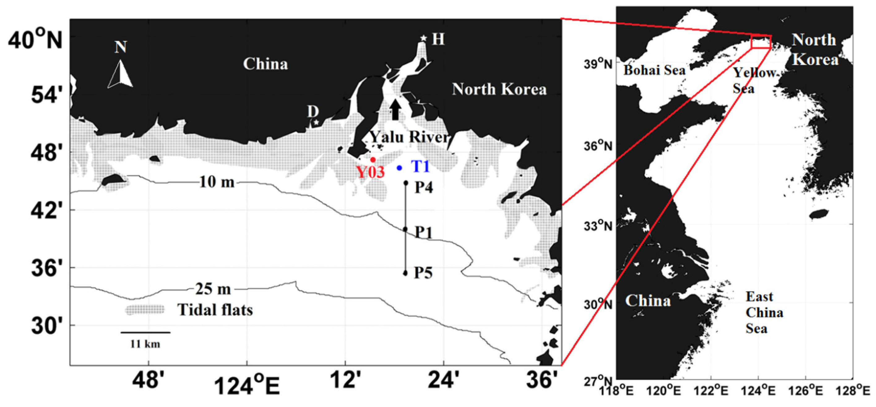
2.1. Study Area
2.2. GOCI Images
2.3. In Situ Data
2.4. Quantitative Retrieval Algorithm of TSM
3. Results and Discussion
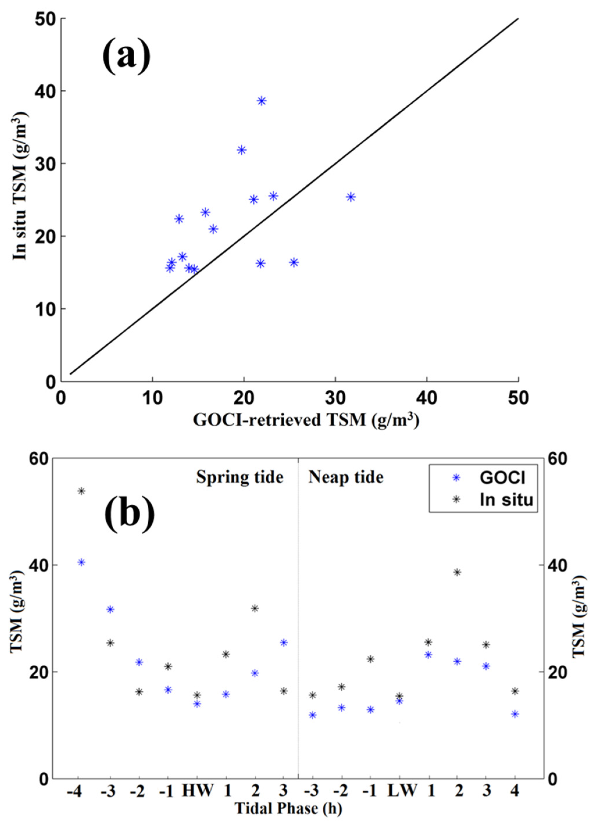
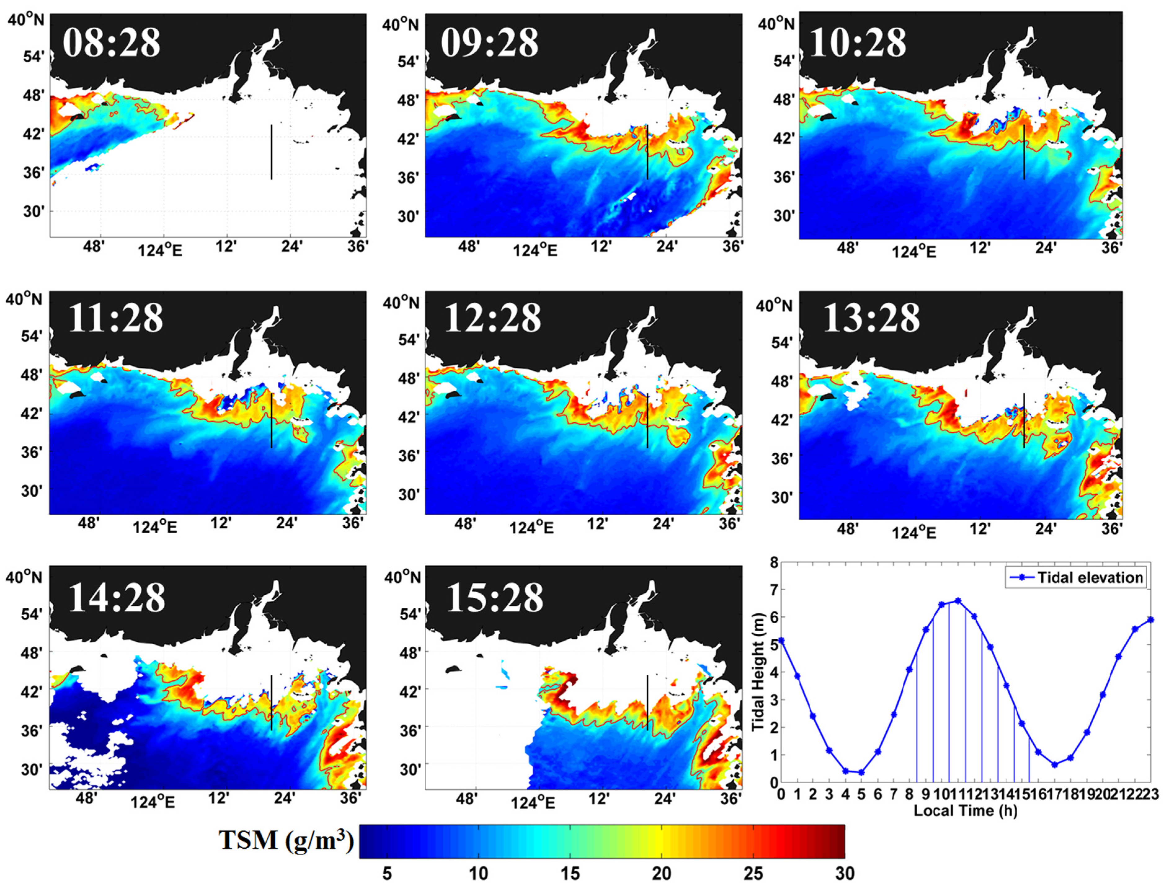
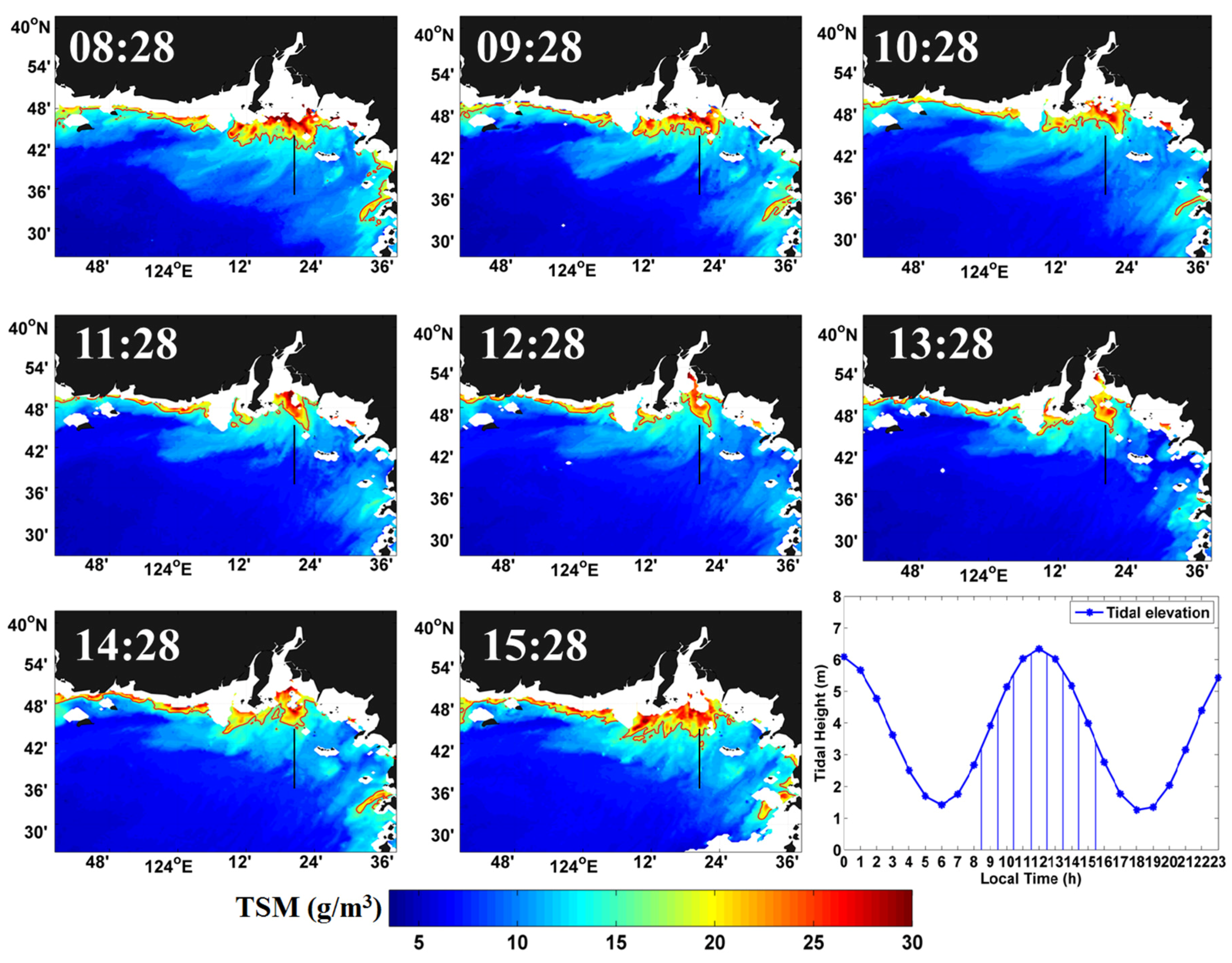
3.1. Diurnal Variation of TSM in the YRE
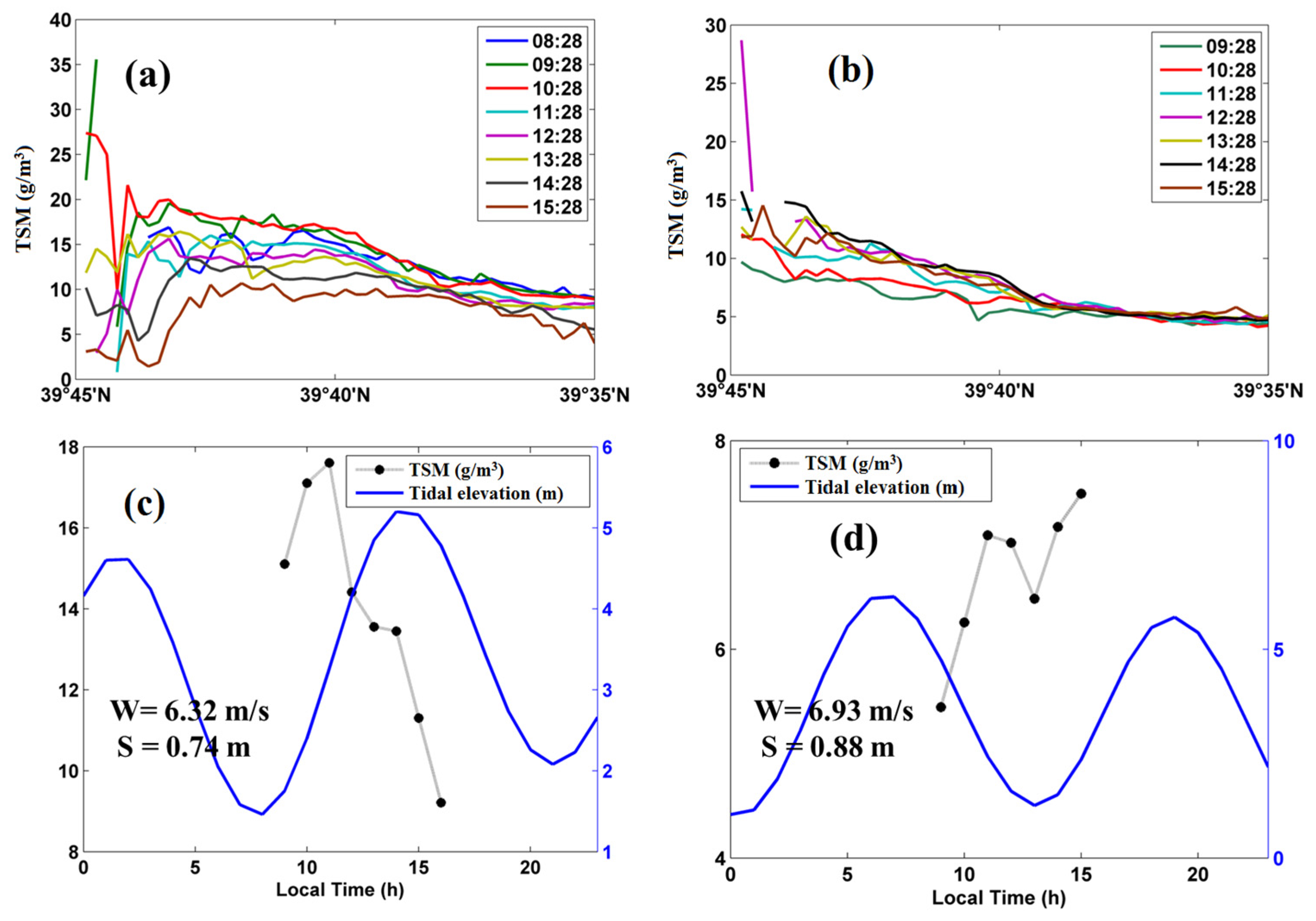
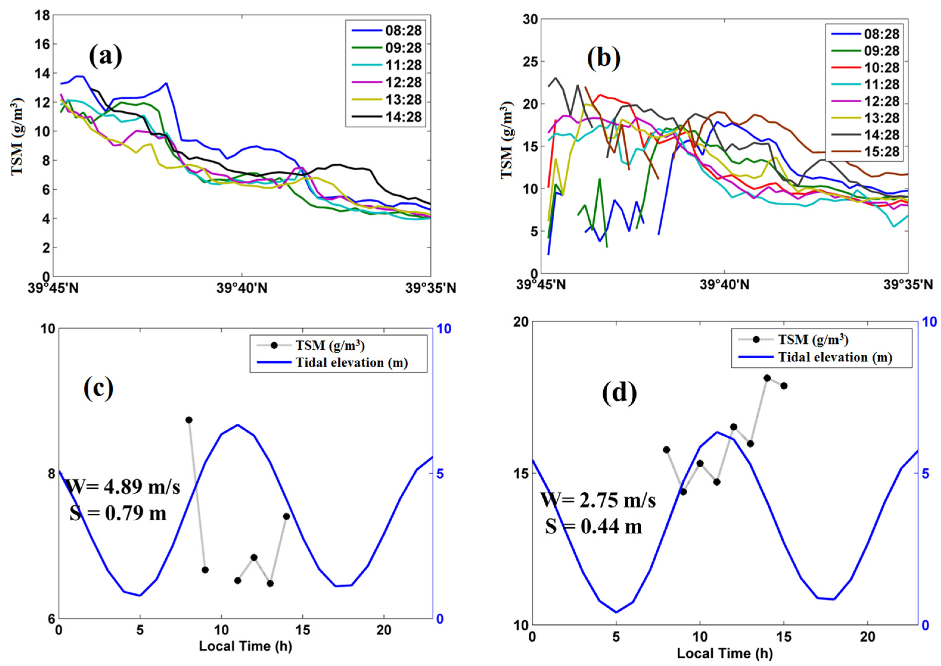
3.2. The Effect of Spring-Neap Tidal Cycle on Diurnal Variation of TSM in the YRE
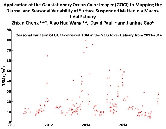
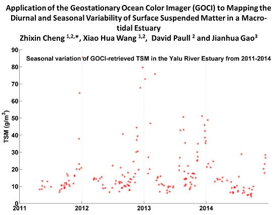
3.3. Seasonal Variation of TSM in the YRE
3.4. Factors Controlling Seasonal Variability of TSM
4. Conclusions
Acknowledgments
Author Contributions
Conflicts of Interest
References
- Neal, C.; Leeks, G.J.L.; Millward, G.E.; Harris, J.R.W.; Huthnance, J.M.; Rees, J.G. Land-ocean interaction: Processes, functioning and environmental management from a UK perspective, an introduction. Sci. Total Environ. 2003, 314–316, 3–11. [Google Scholar] [CrossRef]
- He, X.Q.; Bai, Y.; Pan, D.L.; Huang, N.L.; Dong, X.; Chen, J.S.; Chen, C.-T.A.; Cui, Q.F. Using geostationary satellite ocean color data to map the diurnal dynamics of suspended particulate matter in coastal waters. Remote Sens. Environ. 2013, 133, 225–239. [Google Scholar] [CrossRef]
- Miller, R.L.; McKee, B.A. Using MODIS Terra 250 m imagery to map concentrations of total suspended matter in coastal waters. Remote Sens. Environ. 2004, 93, 259–266. [Google Scholar] [CrossRef]
- Choi, J.-K.; Park, Y.-J.; Lee, B.-L.; Eom, J.; Moon, J.-E.; Ryu, J.-H. Application of the Geostationary Ocean Color Imager (GOCI) to mapping the temporal dynamics of coastal water turbidity. Remote Sens. Environ. 2014, 146, 24–35. [Google Scholar] [CrossRef]
- Ilyina, T.; Pohlmannm, T.; Lammel, G.; Sündermann, J. A fate and transport ocean model for persistent organic pollutants and its application to the North Sea. J. Mar. Syst. 2006, 63, 1–19. [Google Scholar] [CrossRef]
- Gao, S. Fine-grained sediment fluxes and cycling on continental shelves. Forum Young Sch. 21st Century 2000, 22, 73–76. [Google Scholar]
- Tassan, S. Local algorithms using SeaWiFS data for the retrieval of phytoplankton, pigments, suspended sediment, and yellow substance in coastal waters. Appl. Opt. 1994, 33, 2369–2378. [Google Scholar] [CrossRef] [PubMed]
- Zhang, M.; Tang, J.; Dong, J.; Song, Q.; Ding, J. Retrieval of total suspended matter concentration in the Yellow and East China Seas from MODIS imagery. Remote Sens. Environ. 2010, 114, 392–403. [Google Scholar] [CrossRef]
- Shi, W.; Wang, M.; Jiang, L. Spring-neap tidal effects on satellite ocean color observations in the Bohai Sea, Yellow Sea, and East China Sea. J. Geophys. Res. 2011, 116. [Google Scholar] [CrossRef]
- Wang, M.; Ahn, J.-H.; Jiang, L.; Shi, W.; Son, S.H.; Park, Y.J.; Ryu, J.H. Ocean color products from the Korean Geostationary Ocean Color Imager (GOCI). Opt. Express 2013, 21, 3835–3849. [Google Scholar] [CrossRef] [PubMed]
- Liu, X.; Wang, M. River runoff effect on the suspended sediment property in the upper Chesapeake Bay using MODIS observations and ROMS simulations. J. Geophys. Res. Oceans 2014, 119. [Google Scholar] [CrossRef]
- Choi, J.-K.; Park, Y.J.; Ahn, J.H.; Lim, H.-S.; Eom, J.; Ryu, J.-H. GOCI, the world's first geostationary ocean color observation satellite, for the monitoring of temporal variability in coastal water turbidity. J. Geophys. Res. 2012, 117. [Google Scholar] [CrossRef]
- Ryu, J.-H.; Choi, J.K.; Eom, J.; Ahn, J.H. Temporal variation in Korean coastal waters using Geostationary Ocean Color Imager. J. Coast. Res. 2011, SI64, 1731–1735. [Google Scholar]
- Bao, Y.; Tian, Q.J.; Chen, M. A weighted algorithm based on normalized mutual information for estimating the chlorophyll-a concentration in inland waters using Geostationary Ocean Color Imager (GOCI) data. Remote Sens. 2015, 7, 11731–11752. [Google Scholar] [CrossRef]
- Ryu, J.-H.; Han, H.-J.; Cho, S.; Park, Y.-J.; Ahn, Y.H. Overview of Geostationary Ocean Color Imager (GOCI) and GOCI Data Processing System (GDPS). Ocean. Sci. J. 2012, 47, 223–233. [Google Scholar] [CrossRef]
- Lou, X.L.; Hu, C.M. Diurnal changes of a harmful algal bloom in the East China Sea: Observations from GOCI. Remote Sens. Environ. 2014, 140, 562–572. [Google Scholar] [CrossRef]
- Lee, B.R.; Park, Y.J.; Ahn, J.H. Improvement of atmospheric correction for extremely turbid waters using modified MUMM atmospheric correction algorithm. In Proceedings of the International Symposium on Remote Sensing, Ministry of Environment, Incheon, Korea, 10–12 October 2012.
- Ruddick, K.; Vanhellemont, Q.; Yan, J.; Neukermans, G.; Wei, G.M.; Shang, S.L. Variability of suspended particulate matter in the Bohai Sea from the Geostationary Ocean Color Imager (GOCI). Ocean. Sci. 2012, 47, 331–345. [Google Scholar] [CrossRef]
- Yang, H.; Choi, J.K.; Park, Y.J.; Han, H.J.; Ryu, J.H. Application of the Geostationary Ocean Color Imager (GOCI) to estimates of ocean surface currents. J. Geophys. Res. Oceans 2014, 119, 3988–4000. [Google Scholar] [CrossRef]
- Cheng, P.; Gao, S.; Bokuniewicz, H. Net sediment transport patterns over the Northwestern Yellow Sea, based upon grain size trend analysis. Oceanol. Limnol. Sin. 2000, 31, 605–615. [Google Scholar]
- Gao, J.-H.; Gao, S.; Dong, L.X.; Zhang, J. Sediment distribution and suspended sediment transport in Yalu River Estuary. Mar. Sci. Bull. 2003, 22, 27–33. [Google Scholar]
- Yu, Q.; Wang, Y.; Gao, J.; Gao, S.; Flemming, B. Turbidity maximum formation in a well-mixed macrotidal estuary: The role of tidal pumping. J. Geophys. Res. Oceans 2014, 119, 7705–7724. [Google Scholar] [CrossRef]
- Bai, F.L.; Gao, J.H.; Wang, Y.P.; Cheng, Y.; Lin, T.Y. Tidal characteristics at Yalu River Estuary. Mar. Sci. Bull. 2008, 27, 7–13. [Google Scholar]
- State Oceanic Administration. Chinese harbours and embayments: Important estuaries. Ocean 1998, 14, 386–432. (In Chinese) [Google Scholar]
- Seo, S.B.; Lim, H.S.; Ahn, S.I. Introduction to image proper-processing subsystem of Geostationary Ocean Color Imager (GOCI). Korean J. Remote Sens. 2010, 26, 167–173. [Google Scholar]
- Gordon, H.R.; Wang, M. Retrieval of water-leaving radiance and aerosol optical thickness over the oceans with SeaWiFS: A preliminary algorithm. Appl. Opt. 1994, 33, 443–452. [Google Scholar] [CrossRef] [PubMed]
- Wang, M.; Shi, W.; Jiang, L. Atmospheric correction using near-infrared bands for satellite ocean color data processing in the turbid western Pacific region. Opt. Express 2012, 20, 741–753. [Google Scholar] [CrossRef] [PubMed]
- Doxaran, D.; Lamquin, N.; Park, Y.; Mazeran, C.; Ryu, J.H.; Wang, M.; Poteau, A. Retrieval of the seawater reflectance for suspended solids monitoring in the East China Sea using MODIS, MERIS and GOCI satellite data. Remote Sens. Environ. 2014, 146, 36–48. [Google Scholar] [CrossRef]
- Ruddick, K.; Ovidio, F.; Rijkeboer, M. Atmospheric correction of SeaWiFS imagery for turbid coastal and inland waters. Appl. Opt. 2000, 39, 897–912. [Google Scholar] [CrossRef] [PubMed]
- Ahn, J.H.; Park, Y.J.; Ryu, J.H.; Lee, B.; Oh, I.S. Development of atmospheric correction algorithm for Geostationary Ocean Color Imager (GOCI). Ocean. Sci. J. 2012, 47, 247–259. [Google Scholar] [CrossRef]
- Park, Y.-J. GOCI Level 2 Ocean. Color. Products (GDPS 1.3) Brief. Algorithm Description; Korean Ocean Satellite Center: Seoul, Korea, 2014. [Google Scholar]
- Morel, A.; Gentili, B. Diffuse reflectance of oceanic waters, III, Implications of bidirectionality for the remote sensing problem. Appl. Opt. 1996, 35, 4850–4862. [Google Scholar] [CrossRef] [PubMed]
- Morel, A.; Gentili, B.; Antoine, D. Assessing the Atmospheric and Marine Signal. from a Geostationary Orbit; COMS Ocean Data Processing System Development Project: Seoul, Korea, 2005. [Google Scholar]
- Yu, X.; Du, J.B.; Gao, J.H.; Yang, Y.; Ran, L.J.; Li, F.X.; Liu, Y.; Cheng, Y. The influence of hydrodynamic characteristics on the distribution of chlorophy ll concentration in the maximum turbidity of the Yalu Estuary. Acta. Oceanol. Sin. 2012, 34, 101–113. [Google Scholar]
- Son, S.; Wang, M. Water properties in Chesapeake Bay from MODIS-Aqua measurements. Remote Sens. Environ. 2012, 123, 163–174. [Google Scholar] [CrossRef]
- Gordon, H.R.; Brown, O.B.; Evans, R.H.; Brown, J.R.; Smith, R.C.; Baker, K.S.; Clark, D.K. A semi-analytical radiance model of ocean color. J. Geophys. Res. 1988, 93, 909–924. [Google Scholar]
- Kong, J.L.; Sun, X.M.; Wong, D.W.; Chen, Y.; Yang, J.; Yan, Y.; Wang, L.X. A semi-analytical model for remote sensing retrieval of suspended sediment concentration in the gulf of Bohai, China. Remote Sens. 2015, 7, 5373–5397. [Google Scholar] [CrossRef] [Green Version]
- Volpe, V.; Silvestri, S.; Marani, M. Remote sensing retrieval of suspended sediment concentration in shallow waters. Remote Sens. Environ. 2011, 15, 44–54. [Google Scholar] [CrossRef]
- Nechad, B.; Ruddick, K.G.; Park, Y. Calibration and validation of a generic multisensor algorithm for mapping of total suspended matter in turbid waters. Remote Sens. Environ. 2010, 114, 854–866. [Google Scholar] [CrossRef]
- Yu, X.L. Study on Retrieval of Sediment Concentration in Bo and Yellow Sea and Imputation of Missing Value Based on GOCI. Master’s Thesis, Ocean University of China, Qingdao, China, 2013. [Google Scholar]
- Pang, C.; Yu, W.; Yang, Y.; Han, D. An improved method for evaluating the seasonal variability of total suspended sediment flux field in the Yellow and East China Seas. Int. J. Sediment. Res. 2011, 26, 1–14. [Google Scholar] [CrossRef]
- Shi, W.; Wang, M. Satellite views of the Bohai Sea, Yellow Sea, and East China Sea. Prog. Oceanogr. 2012, 104, 30–45. [Google Scholar] [CrossRef]
- Chen, J.; Quan, W.; Cui, T.; Song, Q. Estimation of total suspended matter concentration from MODIS data using a neural network model in the China eastern coastal zone. Estuar. Coast. Shelf Sci. 2015, 155, 104–113. [Google Scholar] [CrossRef]
- Hu, Z.F.; Pan, D.L.; He, X.Q.; Bai, Y. Diurnal variability of turbidity fronts observed by geostationary satellite ocean color remote sensing. Remote Sens. 2016, 8, 147. [Google Scholar] [CrossRef]
- Vaz, J.; Mateus, M.; Dias, J.M. Semidiurnal and spring-neap variations in the Tagus Estuary: Application of a process-oriented hydro-biogeochemical model. J. Coast. Res. 2011, SI64, 1619–1623. [Google Scholar]
- Blanton, J.O.; Seim, H.; Alexander, C.; Amft, J.; Kineke, G. Transport of salt and suspended sediments in a curving channel of a coastal plain estuary: Satilla River, GA. Estuar. Coast. Shelf Sci. 2003, 57, 993–1006. [Google Scholar] [CrossRef]
- Song, D.H.; Wang, X.H. Suspended sediment transport in the Deepwater Navigation Channel, Yangtze River Estuary, China, in the dry season 2009: 2. Numerical simulations. J. Geophys. Res. Oceans 2013, 118, 5568–5590. [Google Scholar] [CrossRef]
- Yu, J. Seasonal Distribution and Variation of Sediments in Yellow Sea. Master’s Thesis, Ocean University of China, Qingdao, China, 2012. [Google Scholar]
- Bai, Y.; He, X.; Pan, D.; Chen, C.-T.A.; Kang, Y.; Chen, X.; Cai, W.-J. Summertime Changjiang River plume variation during 1998–2010. J. Geophys. Res. Oceans 2014, 119, 6238–6257. [Google Scholar] [CrossRef]
- Cheng, Y.; Bi, L.X. Primary character and motive change of shallow beach in Yalu River mouth. J. Sediment. Res. 2002, 3, 59–63. [Google Scholar]
- Gao, J.-H.; Li, J.; Wang, H.; Bai, F.-L.; Cheng, Y.; Wang, Y.-P. Rapid changes of sediment dynamic processes in Yalu River Estuary under anthropogenic impacts. Int. J. Sediment. Res. 2012, 27, 37–49. [Google Scholar] [CrossRef]
- Gao, J.-H.; Gao, S.; Cheng, Y.; Dong, L.; Zhang, J. Formation of turbidity maxima in the Yalu River Estuary, China. J. Coast. Res. 2004, 43, 134–146. [Google Scholar]
- Gao, J.H.; Gao, S.; Cheng, Y.; Dong, L.; Zhang, J. Sediment transport in Yalu river estuary. Chin. Geogr. Sci. 2003, 13, 157–163. [Google Scholar] [CrossRef]
- Wang, X.H.; Pinardi, N. Modeling the dynamics of sediment transport and resuspension in the Northern Adriatic Sea. J. Geophys. Res. 2002, 107, 18:1–18:23. [Google Scholar] [CrossRef]
- Wang, X.H.; Pinardi, N.; Malacic, V. Sediment transport and resuspension due to combined motion of wave and current in the northern Adriatic Sea during a Bora event in January 2001: A numerical modelling study. Cont. Shelf Res. 2007, 27, 613–633. [Google Scholar] [CrossRef]
- Wang, X.H.; Qiao, F.L.; Lu, J.; Gong, F. The turbidity maxima of the northern Jiangsu shoal-water in the Yellow Sea, China. Estuar. Coast. Shelf Sci. 2011, 93, 201–211. [Google Scholar] [CrossRef]
- Song, D.H.; Wang, X.H.; Cao, Z.; Guan, W. Suspended sediment transport in the deepwater navigation channel, Yangtze River Estuary, China, in the dry season 2009: 1. Observations over spring and neap tidal cycles. J. Geophys. Res. Oceans 2013, 118, 5555–5567. [Google Scholar] [CrossRef]


| Date | 9 March | 30 March | 10 March | 21 March |
|---|---|---|---|---|
| Wind Speed (m/s) | 6.32 | 5.63 | 3.05 | 2.75 |
| Significant Wave Height (m) | 0.74 | 0.81 | 0.46 | 0.44 |
| Tidal Range (m) | 3.74 | 5.82 | 3.02 | 4.35 |
| Standard Deviation (g/m3) | 1.29 | 2.54 | 0.75 | 1.93 |
| Date | 3 May | 30 May | 8 June | 14 June |
| Wind Speed (m/s) | 4.89 | 2.57 | 4.06 | 1.07 |
| Significant Wave Height (m) | 0.79 | 0.65 | 0.47 | 0.28 |
| Tidal Range (m) | 3.89 | 5.00 | 2.72 | 6.34 |
| Standard Deviation (g/m3) | 0.96 | 1.40 | 0.66 | 1.13 |
| Month | January | February | March | April | May | June |
|---|---|---|---|---|---|---|
| Wind Speed (m·s−1) | 2.1 | 2.2 | 2.3 | 2.1 | 2.2 | 1.7 |
| Wind Direction | NE | NNE | NNW | SW | SW | SW |
| Month | Jul | Aug | Sep | Oct | Nov | Dec |
| Wind Speed (m·s−1) | 1.7 | 1.6 | 1.8 | 2.1 | 1.9 | 2.3 |
| Wind Direction | WSW | ENE | ENE | ENE | ENE | ENE |
© 2016 by the authors; licensee MDPI, Basel, Switzerland. This article is an open access article distributed under the terms and conditions of the Creative Commons by Attribution (CC-BY) license (http://creativecommons.org/licenses/by/4.0/).
Share and Cite
Cheng, Z.; Wang, X.H.; Paull, D.; Gao, J. Application of the Geostationary Ocean Color Imager to Mapping the Diurnal and Seasonal Variability of Surface Suspended Matter in a Macro-Tidal Estuary. Remote Sens. 2016, 8, 244. https://0-doi-org.brum.beds.ac.uk/10.3390/rs8030244
Cheng Z, Wang XH, Paull D, Gao J. Application of the Geostationary Ocean Color Imager to Mapping the Diurnal and Seasonal Variability of Surface Suspended Matter in a Macro-Tidal Estuary. Remote Sensing. 2016; 8(3):244. https://0-doi-org.brum.beds.ac.uk/10.3390/rs8030244
Chicago/Turabian StyleCheng, Zhixin, Xiao Hua Wang, David Paull, and Jianhua Gao. 2016. "Application of the Geostationary Ocean Color Imager to Mapping the Diurnal and Seasonal Variability of Surface Suspended Matter in a Macro-Tidal Estuary" Remote Sensing 8, no. 3: 244. https://0-doi-org.brum.beds.ac.uk/10.3390/rs8030244