Article

Correction of Incidence Angle and Distance Effects on TLS Intensity Data Based on Reference Targets

1
College of Surveying and Geo-Informatics, Tongji University, NO. 1239, Siping Road, Shanghai 200092, China
2
Department of Land Surveying and Geo-Informatics, The Hong Kong Polytechnic University, Kowloon 999077, Hong Kong, China
*
Author to whom correspondence should be addressed.
Submission received: 7 January 2016 / Revised: 25 February 2016 / Accepted: 4 March 2016 / Published: 16 March 2016

Abstract

:
The original intensity value recorded by terrestrial laser scanners is influenced by multiple variables, among which incidence angle and distance play a crucial and dominant role. Further studies on incidence angle and distance effects are required to improve the accuracy of currently available methods and to implement these methods in practical applications. In this study, the effects of incidence angle and distance on intensity data of the Faro Focus3D 120 terrestrial laser scanner are investigated. A new method is proposed to eliminate the incidence angle and distance effects. The proposed method is based on the linear interpolation of the intensity values of reference targets previously scanned at various incidence angles and distances. Compared with existing methods, a significant advantage of the proposed method is that estimating the specific function forms of incidence angle versus intensity and distance versus intensity is no longer necessary; these are canceled out when the scanned and reference targets are measured at the same incidence angle and distance. Results imply that the proposed method has high accuracy and simplicity in eliminating incidence angle and distance effects and can significantly reduce the intensity variations caused by these effects on homogeneous surfaces.

Graphical Abstract

1. Introduction

Terrestrial laser scanning (TLS), a revolutionary technique for the acquisition of spatial data, has gained widespread acceptance in both scientific and commercial communities as a powerful tool for topographic measurement in various geophysical disciplines in the last two decades [1]. This active remote sensing technique allows for the direct and illumination-independent measurement of 3-D objects in a fast, contactless, non-destructive, and accurate manner [2] by emitting monochromatic beams of light mostly in the near-infrared region of the electromagnetic spectrum. Apart from discrete topography measurements, almost all current TLS instruments simultaneously measure the power of the backscattered laser signal of each point and record it as an intensity value [3]. The intensity recorded by current laser scanners, either in the form of the echo amplitude or full-waveform of the backscattered laser signal [4], can be utilized as complementary information along with the point cloud in a wide range of applications, especially in visualization, segmentation [5], classification [6,7,8,9,10], and multi-temporal analysis [11,12,13,14].
The intensity value is regarded as a significant source of spectral information associated with the surface properties, e.g., reflectance [1,15,16,17,18], roughness [15,19], moisture [11,13,14,20,21], brightness [22,23,24,25] and grain size [26,27], of the scanned object. However, the original intensity data are inapplicable in directly retrieving target features because the intensity detected by TLS systems is affected by at least four essential variables [15], namely, instrumental effects, atmospheric effects, target scattering characteristics, and scanning geometry [28]. Hence, different parts of a homogeneous surface are represented as different values in the measured intensity data. Consequently, intensity data from different instruments and acquisition campaigns are not directly comparable. Intensity values should be corrected before they can be reliably used in applications [29]. TLS intensity correction aims to convert the instrumental (raw) intensity, which is typically not well specified by laser scanner manufacturers, into a corrected value that is proportional or equal to the target reflectance [16,17,18].
For data of a homogeneous surface acquired by the same TLS sensor in one campaign, the major differences in the intensity data are caused by scanning geometry [3,30], that is, the effects of incidence angle and distance (range), given that the instrumental effect is kept constant and atmospheric attenuation is negligible. Therefore, eliminating the effects of distance and incidence angle is indispensable to the extensive application of intensity data.
Theoretically, based on the radar range equation, the intensity of TLS is directly proportional to the cosine of the incidence angle and inversely proportional to the range squared [
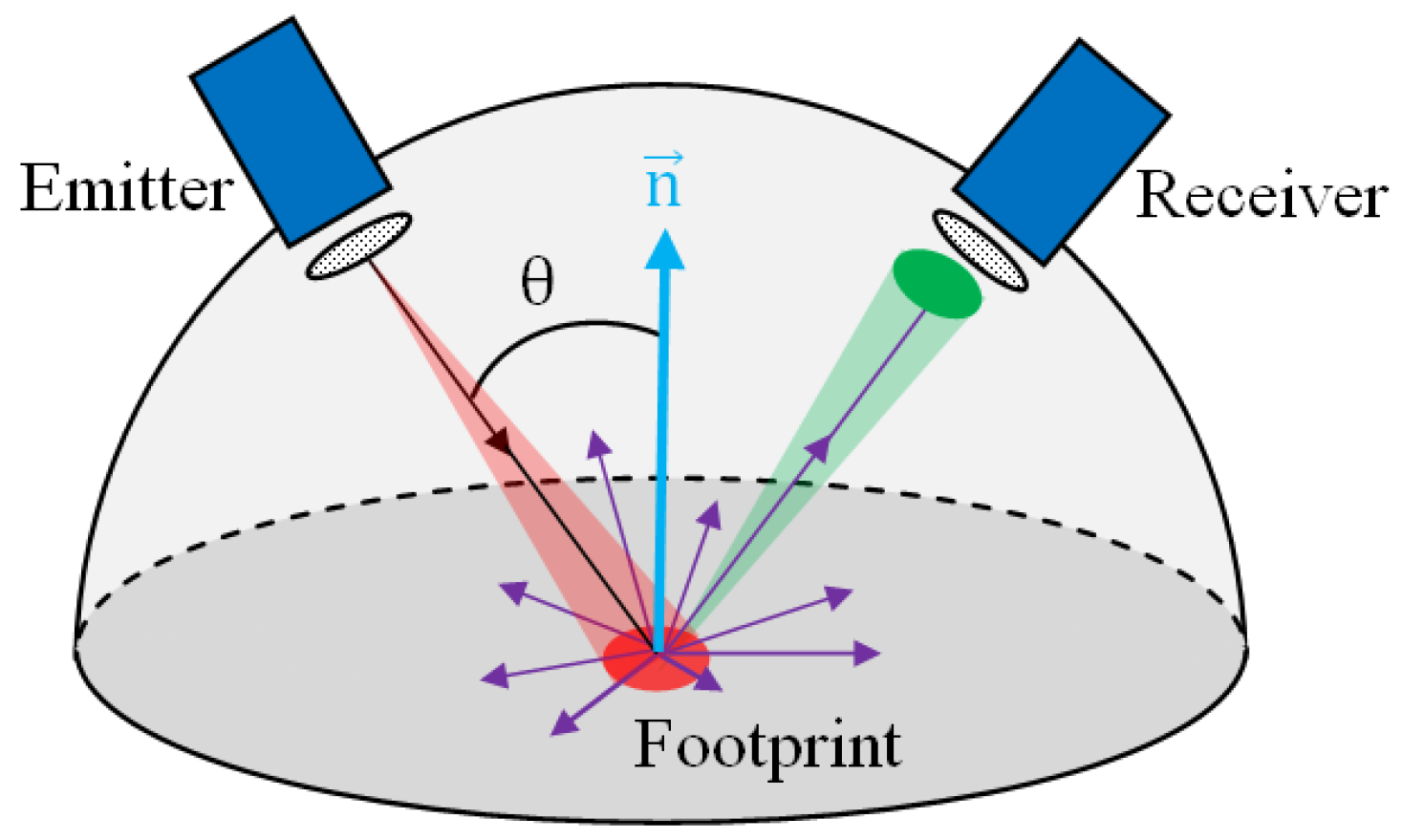
3]. The incidence angle is the angle between beam propagation direction and surface orientation; it is related to target scattering properties, surface structure, and scanning geometry [27]. The interpretation of the incidence angle effect in terms of target surface properties is a complicated task. Lambert’s cosine law can provide a satisfactory estimation of light absorption modeling for rough surfaces in both active and near-infrared spectral domains [31]; thus, it is widely employed in existing intensity correction applications. However, Lambert’s cosine law is insufficient to correct the incidence angle effect for surfaces with increasing irregularity because these surfaces do not exactly follow the Lambertian scattering law [4,27,32].
Range measurements are derived by emitting and receiving laser signals to obtain the time of flight, which allows the distance between the center of the laser scanner and the target to be computed. The distance effect is largely dependent on instrumental properties (e.g., aperture size, automatic gain control (AGC), amplifier for low reflective surfaces, and brightness reducer for near distances [33]) and varies significantly across different laser scanning systems. In reality, the data collected by TLS usually show intensity–range relationships that differ from those in an ideal physical model [3] because the photodetector of TLS is not designed for intensity measurement but for the optimization of range determination. This principle implies that an amplifier may be available for low reflectance and a brightness reducer for near distance [15,18]. More detailed information about the incidence angle and distance effects can be found in [1,3,4,15,16,17,18,22,23,24,25,26,27,28,29,30,31,32,33,34].
In our previous studies [35,36], the incidence angle and distance effects of Faro Focus3D X330 and Faro Focus3D 120 were studied. A polynomial was used to eliminate the incidence angle and distance effects. By contrast, a practical approach based on reference targets with known reflectance properties is developed in this study to correct the distance and incidence angle effects of Faro Focus3D 120. Initial attempts to correct ALS intensity data based on reference targets have been previously exerted [21,37,38,39] where commercially or naturally available reference targets were scanned in situ for the computation of the unknown system parameters. Meanwhile, we aim to correct TLS intensity data based on the linear interpolation of the intensity–incidence angle and intensity–range relationships of the reference targets scanned at various incidence angles and distances. The objectives and contributions of this study are as follows:
  • to provide a short review of recent work on the correction of the incidence angle and distance effects of TLS;
  • to introduce a new method to correct the incidence angle and distance effects on TLS intensity data based on reference targets;
  • to derive relative formulas of the proposed method for linear interpolation of the intensity–incidence angle and intensity–range relationships of the reference targets. Existing correction methods for distance and incidence angle effects in TLS are reviewed in Section 2. The proposed correction model is introduced in Section 3. Section 4 outlines the dataset and experimental results. Section 5 presents and discusses the correction results of the proposed method, and the conclusions are presented in Section 6.

2. Existing Correction Methods

2.1. Radar Range Equation for Extended Lambertian Reflectors

The TLS sensor emits laser pulses at a specific pulse repetition frequency, illuminates the surface objects, and records the returned laser pulse signals after being backscattered from the surface objects [7] (see Figure 1). The entire process follows that of the radar range equation. The equation describes the relationship between the transmitted and received signal power and includes parameters relating to the sensor, the target, and the intervening atmosphere, as follows:
P r = P t D r 2 4 π R 4 β t 2 η sys η atm σ ,
where the received laser power P r is a function of the transmitted power P t , the receiver aperture diameter D r , the distance R from the sensor to the target, the laser beam width β t , the system transmission factor η sys , the atmospheric transmission factor η atm , and the target cross-section σ .
The case of an extended target where the target surface is usually larger than the laser footprint size can be considered in TLS. The actual light reflection behaviors of the scanned surfaces are very complicated. To simplify the reflection model, the scanned target is always assumed to possess Lambertian characteristics [16]. For Lambertian reflectors, the entire surface reflects laser shots by Lambert’s cosine law, such that an incident ray is reflected to a hemisphere uniformly (see Figure 1) rather than at only one angle as in the case of specular reflection. The intensity observed from a Lambertian surface is directly proportional to the cosine of the angle between the observer’s viewing direction and the surface normal. Considering that the light paths from the emitter and detector coincide in TLS, the received laser power is proportional to the cosine of the incidence angle. For extended Lambertian reflectors, the radar range equation is provided by [16]:
P r = P t D r 2 ρ cos θ 4 R 2 η sys η atm ,
where ρ is the reflectance of the scanned target and θ is the incidence angle.
Given that laser scanning data are collected by the same sensor, all sensor-related factors (i.e., P t , D r , and η sys ) can be assumed as constant for a certain system during one campaign [3]. In TLS, the atmospheric transmission effect can usually be neglected [3,15,18]. Therefore, Equation (2) can be further simplified as:
P r = C   ×   ρ   ×   cos θ   × R 2 ,
where C = P t D r 2 η sys / 4 which is an unknown but constant parameter for a specific scanner.

2.2. Existing Correction Methods for Distance and Incidence Angle Effects

The intensity value is a measure of the electronic signal strength obtained by converting and amplifying the backscattered optical power [40]. This condition indicates that the left side of Equation (3) is converted into a voltage, amplified in the system, and finally transformed into a digital number (DN), that is, a scaled integer value, through an unknown proprietary function [16]. Further specification of the processing steps of received power P r is not disclosed. The intensity value is generally proportional to the number of photons impinging on the detector in a specific time interval [1], that is,
I P r ρ   ×   cos θ   × R 2
Although Equation (4) is a simplified mathematical law and the light scattering behaviors of most natural surfaces are not Lambertian, many studies have reported that incidence angle dependence for many surfaces approximately follows the cos θ relation [4,7,8,15,16,17,18]. However, the accuracy of the correction of the incidence angle effect can be further improved. The distance effect correction method in Equation (4) can be applied to TLS but not at all ranges [3,15,18,25]. Furthermore, considering the fact that the incidence angle and distance effects are theoretically independent of each other and can be solved separately [3,27], the theoretical incidence angle effect ( cos θ ) and distance effect ( R 2 ) in Equation (4) are replaced with f 2 ( cos θ ) that is a function of the incidence angle and f 3 ( R ) that is a function of the distance, respectively, as shown in Equation (5) in this study.
I = f 1 ( ρ ) × f 2 ( cos θ ) × f 3 ( R )
According to the definition of intensity correction, the corrected intensity value I s , which is independent of the distance and incidence angle and is only related to the target reflectance, is derived as follows:
I s = f 1 ( ρ ) = I / [ f 2 ( cos θ ) · f 3 ( R ) ]
TLS intensity is a complicated function of incidence angle and distance. Various models of f 2 ( cos θ ) and f 3 ( R ) have been proposed to correct the distance and incidence angle effects in TLS. To improve the correction of laser scanning intensity data, a revised version of Equation (4) called the extended Lambertian reflection model [41] is proposed to modify the contribution of incidence angle and distance by changing the constant exponential values to parameters that are derived from the experimental data. Considering that non-Lambertian behavior occurs in some natural surfaces, a model that is a linear combination of the Lommel–Seeliger law pertaining to intrinsically dark surfaces and the Lambertian law relating to bright targets is applied to correct the incidence angle effect [3,15]. Given that in most cases diffuse and specular reflections exist simultaneously in natural surfaces, the empirical Phong reflection model, which describes the way a surface reflects light as a combination of both diffuse and specular forms, is proposed to eliminate the incidence angle effect [29,41].
Given the existence of detector effects at the entire range scale, Kaasalainen et al. [15] suggested after an extensive analysis and study of the TLS distance effect that the most suitable means for distance effect correction is the use of a reference table. In this case, the correction values are determined by external reference measurements. However, no specific method was given. Under the condition that sufficient information on the detector operation and characteristics is available, a previous study [18] conducted distance effect correction with external reference targets where the measurements of a near-infrared camera were used for the validation. Based on Equation (4), Fang et al. [3] reported that the near distance effect in TLS is caused by the defocusing effect of the receiver’s optics and theoretically derived the formula of f 3 ( R ) which perfectly settled the near-distance effect. However, the parameters should be estimated in accordance with observed values by iterative curve fitting using a nonlinear least squares method and robust Gauss-Newton algorithm. With practical intensity–range data, several studies empirically substituted f 3 ( R ) with the piecewise linear model [40,42,43]. Given the complexity of the incidence angle and distance effects in TLS, a polynomial was adopted to approximately substitute both f 2 ( cos θ ) and f 3 ( R ) to the maximum extentwith very satisfactory results in our previous studies [35,36]. However, the polynomial parameters should be estimated individually for different instruments. Besides, it is even difficult to find an appropriate polynomial to substitute f 3 ( R ) for some instruments because of the complicated and irregular distance effect.

3. Proposed Model for Intensity Correction

As stated above, estimating the specific forms of f 2 ( cos θ ) and f 3 ( R ) is indispensiable for most of the existing methods. This is a tough task and the derived models may lack versatility as f 2 ( cos θ ) and f 3 ( R ) are complicated and vary significantly in different scanners. Nevertheless, the distance effect mainly depends on the instrument effects which can be neutralized by using reference targets. The incidence angle effect is primarily caused by the surface properties; thus, the incidence angle effect differs for various targets. Though most targets found in nature are not Lambertian, the light scattering behavior of most natural surfaces approximately exhibits Lambertian attributes. Therefore, f 2 ( cos θ ) and f 3 ( R ) are unchanged for a specific instrument, i.e., the values of f 2 ( cos θ ) and f 3 ( R ) are the same for different targets if they are scanned at the same incidence angle and distance regardless of the specific details of how the intensity value is measured and recorded. This condition means that the incidence angle and distance effects can be neutralized when the scanned and reference targets are measured at the same scanning geometry even though the specific forms of f 2 ( cos θ ) and f 3 ( R ) are unknown, i.e., the estimation of f 2 ( cos θ ) and f 3 ( R ) is avoidable. The fundamental principles of the proposed method are introduced as follows.
In a small section, f 2 ( cos θ ) and f 3 ( R ) can be considered linear functions. Thus, linear interpolation can be utilized to obtain the intensity values within this small section; however, a monotonic relationship must be made between the recorded intensity and the variables (incidence angle or distance) [3]. If a reference target with reflectance ρ s is scanned at various incidence angles and at a constant distance R s , i.e., the incidence angles satisfy
a = cos θ 0 < cos θ 1 < < cos θ m = b ,
the relationship between incidence angle and intensity can be obtained.
If an incidence angle θ x satisfies
cos θ i < cos θ x < cos θ i + 1 , i = 0 , 1 , , m 1 ,
I ( ρ s , cos θ x , R s ) can be calculated based on a linear interpolation between ( N i , M i ) and ( N i + 1 , M i + 1 ) as shown below.
I ( ρ s , cos θ x , R s ) = M x = M i + 1 M i N i + 1 N i ( N x N i ) + M i ,
where
{ M i + 1 = I ( ρ s , cos θ i + 1 , R s ) M i = I ( ρ s , cos θ i , R s ) N i + 1 = cos θ i + 1 N i = cos θ i N x = cos θ x
Similarly, the intensity value at incidence angle θ s can be interpolated as follows:
I ( ρ s , cos θ s , R s ) = M s .
Furthermore, if this reference target is scanned at multiple distances and at an identical incidence angle θ s , i.e., the distances satisfy
c = R 0 < R 1 < < R n = d ,
the relationship between distance and intensity can be acquired.
If a distance satisfies
R j < R y < R j + 1 ,   j = 0 , 1 , , n 1 ,
I ( ρ s , cos θ s , R y ) can be calculated based on a linear interpolation between ( V j , U j ) and ( V j + 1 , U j + 1 ) as shown below.
I ( ρ s , cos θ s , R y ) = U y = U j + 1 U j V j + 1 V j ( V y V j ) + U j ,
where
{ U j + 1 = I ( ρ s , R j + 1 , cos θ s ) U j = I ( ρ s , R j , cos θ s ) V j + 1 = R j + 1 V j = R j V y = R y .
Similarly, the intensity at distance R s can be interpolated as
I ( ρ s , cos θ s , R s ) = U s
By combining Equations (11) and (16), we have
I ( ρ s , cos θ s , R s ) = ( M s + U s ) / 2
According to Equation (5), Equations (9), (14), and (17) can be written as:
{ I ( ρ s , cos θ x , R s ) = f 1 ( ρ s ) × f 2 ( cos θ x ) × f 3 ( R s ) I ( ρ s , cos θ s , R y ) = f 1 ( ρ s ) × f 2 ( cos θ s ) × f 3 ( R y ) I ( ρ s , cos θ s , R s ) = f 1 ( ρ s ) × f 2 ( cos θ s ) × f 3 ( R s )   .
Besides, the intensity of the reference target scanned at incidence angle θ x and distance R y according to Equation (5) is
I ( ρ s , cos θ x , R y ) = f 1 ( ρ s ) × f 2 ( cos θ x ) × f 3 ( R y ) .
According to Equations (9), (14), (17–(19) is equal to
I ( ρ s , cos θ x , R y ) = I ( ρ s , cos θ x , R s ) ×   I ( ρ s , cos θ s , R y ) I ( ρ s , cos θ s , R s ) = 2 × M x × U y M s + U s .
For a target with unknown reflectance ρ scanned at incidence angle θ x and distance R y , the original recorded intensity is I ( ρ , cos θ x , R y ) which satisfies
I ( ρ , cos θ x , R y ) = f 1 ( ρ ) × f 2 ( cos θ x ) × f 3 ( R y )
According to Equations (19) and (21),
I ( ρ s , cos θ x , R y ) I ( ρ , cos θ x , R y ) = f 1 ( ρ s ) f 1 ( ρ ) = I s ( ρ s ) I s ( ρ ) .
Therefore, the corrected value of this target is
I s ( ρ ) = f 1 ( ρ ) = f 1 ( ρ s ) × I ( ρ , cos θ x , R y ) I ( ρ s , cos θ x , R y ) .
In Equation (23), I ( ρ s , cos θ x , R y ) can be calculated, as shown in Equation (20). I ( ρ , cos θ x , R y ) is the original measured intensity value, and f 1 ( ρ s ) (i.e., I s ( ρ s ) ) can be estimated by the reference target. The corrected intensity value is obtained by a reference target scanned at the same scanning geometry so that the effects of incidence angle and distance can be neutralized under the condition that the intensity is merely related to the reflectance when the incidence angle and distance are the same. In summary, to correct the intensity value of a certain point scanned at θ x and R y , we should firstly obtain the interpolated intensity value of the reference target at θ x and R y by the monotonic relationships of incidence angle versus intensity and distance versus intensity of the reference target.
For relative correction [17], only a value related to the reflectance should be acquired so that f 1 ( ρ s ) can be arbitrarily defined; this scenario means that the corrected intensity value calculated by Equation (23) is relative but comparable. Selecting different reference targets leads to different relative correction results. However, for absolute correction that aims to produce intensity values equal to the reflectance [17], f 1 ( ρ s ) should be estimated by the reference target with known reflectance; the absolute correction results are independent of the reference target.
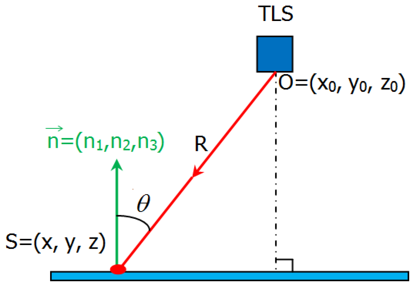
The incidence angle can be calculated by the instrument and object positions as well as surface orientation. Estimation of surface orientation is implemented by computing the best-fitting plane with the available data on the nearby neighborhood of each measured laser point. The incidence angle and distance are derived as follows:
{ R = ( x x 0 ) 2 + ( y y 0 ) 2 + ( z z 0 ) 2 cos θ = | OS n R   × | n | | ,
where n ( n 1 , n 2 , n 3 ) is the normal vector.The incidence radiation vector OS = ( x x 0 , y y 0 , z z 0 ) is calculated with the original geometrical coordinates ( x , y , z ) of the point and the coordinates ( x 0 , y 0 , z 0 ) of the scanner center, as shown in Figure 2. Given that the incidence angles can be negative or greater than 90° because of the direction of vectors, these values are converted into a range between 0° and 90° by introducing an absolute operator, as shown in Equation (24).
To evaluate the results of the correction of the incidence angle and distance effects, the coefficient of variation, which can eliminate the influence of the numerical scale, of the intensity values of a homogeneous surface before and after correction, is selected as a measure of quality [16,41]. The coefficient of variation is defined as
CV = σ μ ,
where μ is the mean value and σ is the standard deviation. CV ori and CV cor are set as the coefficient of variation of the original and corrected intensity values, respectively. If the parameter
ε = CV cor / CV ori
is less than 1, the correction model is effective. A small ε leads to good correction results.

4. Incidence Angle and Distance Experiments

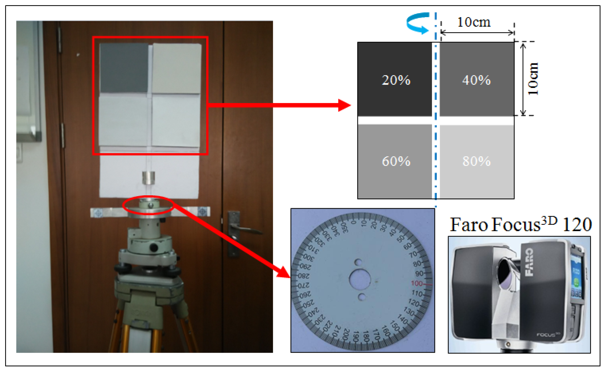
Two sets of experiments were conducted with four Lambertian targets to establish a reference for the interpolation of the incidence angle and distance effects. As indicated in Figure 3, the four reference targets with a size of 10 cm × 10 cm and reflectance of 20%, 40%, 60%, and 80% were mounted on a board. The board was installed on a tripod through a metal stent, on which a goniometer that enables the board to rotate horizontally was placed. The experiments were conducted under laboratory conditions through the use of the Faro Focus3D 120 terrestrial laser scanner, which delivers geometrical information and return intensity values recorded in 11 bits (0 2048). The main system parameters of the scanner are listed in Table 1.
The first set of experiments was implemented at a fixed distance of 5 m from the scanner and rotated in steps of 5° from 0° to 80° to provide a reference for the interpolation of the incidence angle effect. In each orientation step, the board was scanned and all other variables except the incidence angle were considered unchanged. In the second set of experiments, the distance to the board was varied at a fixed incidence angle to establish a reference for the interpolation of the distance effect. The board was perpendicular to the scanner to minimize the influence of the incidence angle on the intensity values. For Faro Focus3D 120, the distance effect is complicated at near distances; thus , the board was placed at a distance range of 1 m–5 m (in intervals of 1 m) and 5 m–29 m (in intervals of 2 m). Empirically, the scanned data of Faro Focus3D 120 above 30 m are unreliable in practical applications because of the low accuracy, large amount of noises, and high level of uncertainties, although the maximum distance is 120 m. Thus, experiments on longer distances were not conducted in this study.
For the two sets of experiments, the scan quality and scan resolution was set to 4 and 1/4, respectively, with a default of view of 360° × 305°. The original recorded intensity values were extracted in a point cloud image created by the standard software Faro SCENE 4.8. A total of 17 scans for each of the two sets of experiments were obtained, containing between 51 and 16,226 points per scan depending on the orientation of the board with respect to the laser beam and the distance between the scanner and the board. For different parts of the same target, TLS intensity is determined by the incidence angle and distance according to Equation (7) given that the reflectance is the same. In a small region of a homogeneous target, the differences in intensity data are minimal given that the incidence angles and distances are nearly the same. In this study, the size of all the four Lambertian targets is 10 cm × 10 cm; the standard deviations of the original intensity data per target are in the range (6.02, 19.07). Therefore, the average intensity value over a selected surface area of each target was used for the analysis. The surface data of the targets were manually sampled as fully as possible; additional uncertainty may be caused by mixed pixels. The proposed method was tested and run in MATLAB programming language.
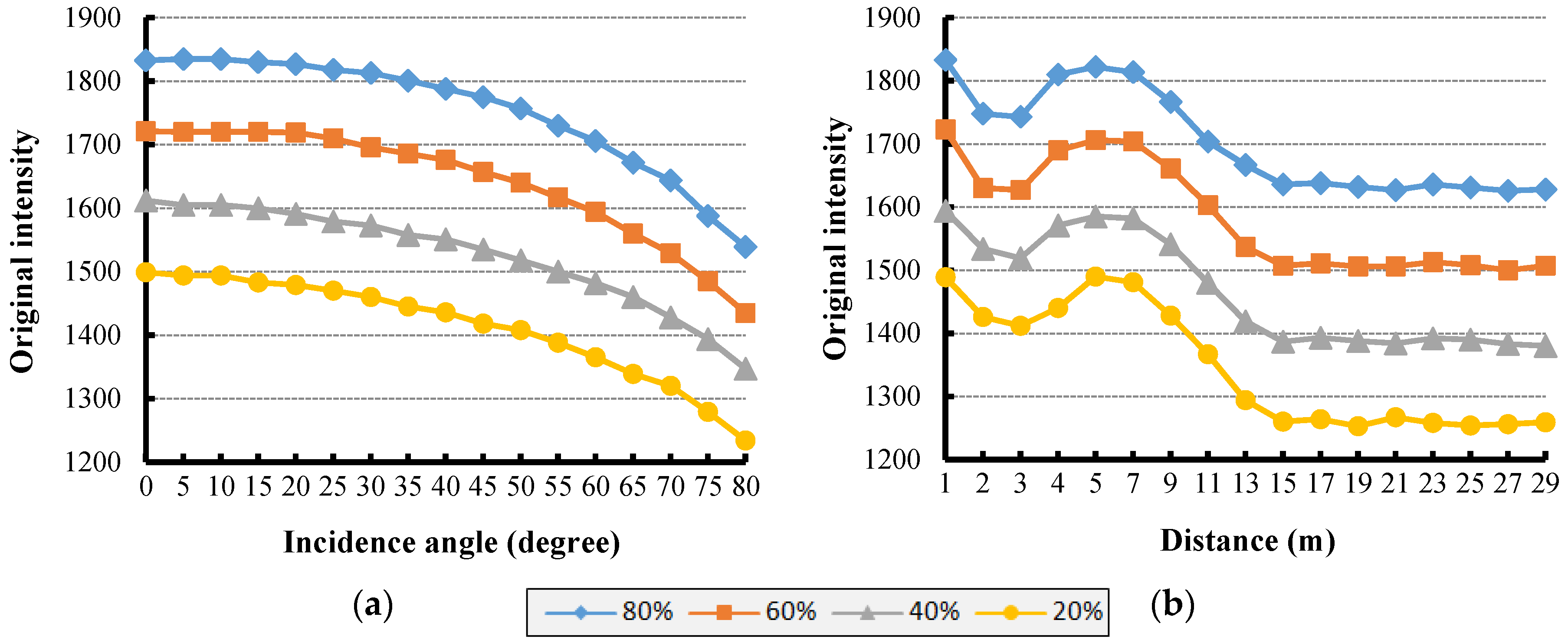
The results of the first set of experiments are shown in Figure 4a. The incidence angle effect is visible, and the curves for different targets have the same features. The overall trend is that for the same target at a fixed distance, the intensity value decreases as the incidence angle increases. However, we tested the relationship between incidence angle and intensity in Figure 4a and found that the relationship does not fit the standard Lambert’s cosine law. A constant and an offset of the cosine of the incidence angle should be added for more accurate results, as suggested by [15]. Even if the incidence angle effect follows the standard Lambert’s cosine law, i.e., the plot lines in Figure 4a are separate in the zero angle of incidence and eventually become very close in larger angles till they all reach zero intensity at 90 degrees, this does not influence our proposed method. The ratio of intensity values measured on two targets with different reflectance is a constant number as long as they are measured with the same scanning geometry regardless of the function forms of f 2 ( cos θ ) and f 3 ( R ) . For small incidence angles from 0° to 30°, the intensity declines slightly, as previously confirmed in [21,30,32]. Afterward, the intensity decreases considerably. For different targets, the intensity values acquired at different incidence angles may be equal. This condition indicates that the incidence angle significantly affects the original recorded intensity. Therefore, to exploit the intensity data, the incidence angle effect of TLS must be eliminated.
The results of the second set of experiments are shown in Figure 4b. The near- and large-distance effects are apparent, and the curves of different targets are consistent. Specifically, the original intensity decreases for short distances below 3 m (i.e., drastically from 1 m to 2 m and then marginally from 2 m to 3 m). Thereafter, the intensity increases significantly from 3 m to 5 m, followed by a steep decrease from 5 m to 15 m. Finally, the intensity begins to level out for ranges over 15 m. For different targets, the intensity values acquired at different ranges may be similar. This similarity indicates that intensity largely depends on distance. Consequently, the distance effect should be eliminated. The detectors of Faro scanners are not designed for intensity measurement, but rather to optimize the range determination [18]. Therefore, a logarithmic intensity scale always exists in Faro scanners. To get the raw intensity values into a linear scale, previous studies [18,25] employed a logarithmic correction to correct logarithmic amplifier effects of Faro scanners(similar to the scanner used in this study). However, we did not specially take the logarithmic amplifier effect into consideration in this study because the kind of instrumental effects of the logarithmic amplifier are effects which are independent of the target properties. No matter what the instrumental effects are, they are the same for different targets and can be neutralized by using reference targets.
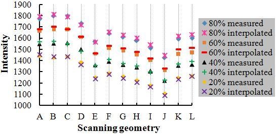
Both of the two sets of experiments reveal that intensity is proportional to reflectance when incidence angle and distance are the same. This condition indicates that the intensity values of different targets scanned at the same scanning geometry are directly comparable, as shown in Equation (22). The feasibility of the proposed method is revealed by the result that the intensity approximately follows a linear trend in an adjacent section of the incidence angle and distance, as shown in Figure 4.

5. Results and Discussion

5.1. Comparisons of Measured and Interpolated Intensity Values

To validate the proposed correction method, we scanned the boardat other scanning geometries (in steps of approximately 2–3 m with a random orientation with respect to the board) referred to A–L, as shown in Table 2. The distances and incidence angles were calculated according to Equation (24). The measured intensity values of the four reference targets at scanning geometries A–L are presented in Figure 5.
Theinterpolated intensity values of the four reference targets at scanning geometry A–L can be calculated according to Equation (20). For example, the calculation process of the interpolated intensity value of the 80% target at scanning geometry A is depicted as follows.
  • First, according to Equation (9) and Figure 4a, the intensity value of the 80% target at 7.6° was interpolated between the intensity values at 5° and 10°.
  • Second, according to Equation (14) and Figure 4b, the intensity value of the 80% target at 1.54 m was interpolated between the intensity values at 1 m and 2 m.
  • Finally, the intensity value of the 80% target at 7.6° and 1.54 m according to Equation (20) was calculated as 1794; the measured intensity value of the 80% target at 7.6° and 1.54 m was 1772. The measured and interpolated intensity values were approximately equivalent.
Similarly, the interpolated intensity values of other targets at other scanning geometries were calculated, as shown in Figure 5 and Table 3. Visually, the measured intensity values optimally fit the ones interpolated from Figure 4a,b. Quantitatively, the mean value of the differences between the measured and interpolated intensity values in Table 3 is 15.02 and the root mean square error (RMSE) is 17.52, which proves that the proposed method exhibits high accuracy in estimating intensity data.

5.2. Correction Results of Reference Targets

The 80% target scanned in the incidence angle and distance experiments (shown in Figure 4a,b) was selected as a reference to correct the intensity data measured at scanning geometries from A to L, as shown in Figure 5. If the corrected intensity values of the 80% target were set equal to the original intensity value of the 80% target at distance 5 m and incidence angle 0°, i.e., I ( ρ s ) = 1833 , the corrected intensity values of the four targets at scanning geometries A–L were calculated according to Equation (23), as shown in Figure 6a.
For example, the intensity value of the 80% target at scanning geometry C (distance 6.88 m and incidence angle 33.3°) was interpolated as 1792, whereas that of the 20% target at distance 6.88 m and incidence angle 33.3° was measured as 1437, as shown in Table 3. Thus, according to Equation (23), the corrected intensity value of the 20% target at scanning geometry C is 1470.
The corrected intensity values when the 60% ( I ( ρ s ) = 1640), 40% ( I ( ρ s ) = 1500), and 20% ( I ( ρ s ) = 1470) targets are selected as reference targets are presented in Figure 6b–d, respectively.
A comparison of Figure 5 and Figure 6 provides the following conclusions. Before correction, intensity is influenced by incidence angle and distance, and differences exist in the raw intensity values for the same target acquired at various incidence angles and distances. After correction, the intensity values do not depend on incidence angle and distance and are solely associated with reflectance; the differences in intensity values acquired at various incidence angles and distances of the same target are negligible. However, the corrected intensity values of the same target are unequal when different reference targets are selected because the corrected intensity value of the reference target I ( ρ s ) ( f 1 ( ρ s ) ) can be arbitrarily defined for relative correction. This finding implies that the corrected intensity values are related to but not equal to the reflectance of the scanned target. The quantitative results of relative correction are presented in Table 4. The table shows that the mean values of ε are approximately 0.19, 0.13, 0.13, and 0.20 for Figure 6a–d, respectively. All of these values are much smaller than 1. This result suggests that the proposed method can effectively eliminate incidence angle and distance effects on original intensity data. Empirically, the relationship between corrected intensity and true reflectance is somehow an "S" curve. As shown in Figure 6, in the middle range, it is close to linear and matches with our linear calibration procedure, whereas in the two side ranges it may be non-linear.
For absolute correction, the function form of f 1 ( ρ ) should be determined. As indicated in Figure 4a,b, the intensity is proportional to the reflectance when the incidence angle and distance are the same. f 1 ( ρ ) was estimated as
f 1 ( ρ ) = ρ + 2.1851
for Faro Focus3D 120. The method for estimating f 1 ( ρ ) was introduced in detail in our previous study [36]. Therefore, Equation (23) can be rewritten as
I s = ρ = ( ρ s + 2.1851 ) × I ( ρ , cos θ x , R y ) I ( ρ s , cos θ x , R y ) 2.1851
The intensity values absolutely corrected according to Equation (28), i.e., the reflectance values, are shown in Table 5. The mean corrected intensity values of the four targets using different reference targets are approximately equal and close to the true reflectance values. By setting ρ i as the recovered reflectance from Equation (28) and ρ 0 as the known reflectance, the mean error of the reflectance retrieval of N targets is calculated as
δ = i = 1 N | ρ i ρ 0 | N × 100 % .
According to the data in Table 5, δ is 3.68%. This result suggests that the proposed method has high accuracy.

5.3. Correction Results of Natural Targets

To further investigate the applicability of the proposed method, the results of the proposed method on natural surfaces were analyzed. The Faro Focus3D 120 scanner was utilized to scan a white lime wall, a building facade with gray bricks, and a cement road. The surface roughness is approximately 0.1 mm–0.2 mm, 0.8 mm–1.5 mm, and 0.5 mm–1.0 mm for the wall, building, and road, respectively. The original intensity images of the three surfaces are shown in Figure 7a–c. A total of 20 small regions with a size of approximately 15 cm × 15 cm in the three surfaces, with different incidence angles and distances, were manually and randomly sampled.
The mean original intensity values, distances, and cosine on incidence angles of the selected regions are shown in Figure 7d–f, respectively. Of course, the effects of errors and outliers cannot be observed if we use mean intensity values, and the way someone select the regions (e.g., mixed pixels) may have a slight influence on the accuracy calculated at the end. But, these effects are minimal and may be neutralized if we use the mean intensity value. These 20 small regions with different incidence angles and distances were randomly selected from different parts of the three surfaces. The regions are typical to some extent. If we randomly and arbitrarily choose 20 small regions from three different surfaces, the proposed method is effective. This can prove the feasibility of our proposed method. The field test may not be ideal but can well suppose the validation of the proposed method. The relative correction results of the three surfaces obtained by using different reference targets are shown in Figure 8, where f 1 ( ρ s ) is set as 1833, 1640, 1500, and 1470 for the 80%, 60%, 40%, and 20% reference target, respectively.
As shown in Figure 7d, the original intensity is influenced by the incidence angle and distance. As such, the intensity values of different regions of the same target differ significantly although they have the same scattering property. Excessive overlaps occur in the original intensity values for the three targets. Nevertheless, the relatively corrected intensity values of different regions of the same target are approximate, as shown in Figure 8. Distinguishing these targets based on the corrected intensity values is feasible. The quantitative results of relative correction are presented in Table 6. The mean values of ε are approximately 0.16, 0.13, 0.11, and 0.20 for Figure 8a–d, respectively. This result proves the feasibility of the proposed method on natural surfaces.
The absolute correction results are shown in Figure 9 and Table 7. The mean corrected intensity values (reflectance) obtained using different reference targets are approximately equal. To evaluate the results quantitatively, we utilized the FieldSpec Pro spectrometer manufactured by Analytical Spectral Devices Inc. to measure the reflectance values of the three surfaces. The reflectance values of the three surfaces measured by the spectrometer at a wavelength of 905 nm are 78%, 49%, and 27%, which are considered true reflectance values (each surface was measured ten times to obtain the mean reflectance). Compared with the reflectance values measured by the spectrometer, the value of δ is 3.09%. This also proves the high accuracy of the proposed method on natural surfaces.
As shown in Figure 8 and Figure 9, several errors were detected in the corrected intensity values. These errors can be explained by the following points. From a theoretical perspective, the proposed method depends on the assumption that the systematic parameters are constant during the entire campaign. However, this condition may be untrue for several laser sources. For example, the emitted power P t can change because of environmental factors, such as temperature. From a practical perspective, environmental effects and variations in surface property affect the accuracy of the proposed method. For example, the dust and dirt on the road, the internal moisture content, the grout between the bricks, or the external erosion of the wall, will change the surface reflectance properties, that is, the scanned surface is not exactly homogeneous at every part. Furthermore, several measuring errors may exist in the reference targets which would also lead to variations in the corrected intensity values.
To further prove the superiority of the proposed method, the polynomial method [36] was applied to correct the incidence angle and distance effects of the sampled data of the three natural surfaces. The specific forms of f 2 ( cos θ ) and f 3 ( R ) for Faro Focus3D 120 are listed in Table 8. The polynomial degree was set as 3 and 8 for f 2 ( cos θ ) and f 3 ( R ) , respectively, to maintain balance in the simplicity and accuracy of the model. The polynomial coefficients were estimated by least squares adjustment. The absolute correction results (reflectance) of the three surfaces by the polynomial method are 76.82%, 51.34%, and 26.51%, similar to that of the proposed method. Compared with the results of the spectrometer, the value of δ is 2.25% for the polynomial method. Even though the correction results of the polynomial method is 0.84% higher than that of the proposed method, the estimation of the polynomial parameters is a tough task. Additionally, the accuracy of the spectrometer and the number of sampled regions should be considered for a more reasonable comparison between the polynomial method and the proposed method. Furthermore, it should be noted that for some TLS systems with a complex distance effect, the polynomial method may be invalid. Therefore, we can conclude that without estimating the specific forms of f 2 ( cos θ ) and f 3 ( R ) , the accuracy of the proposed method is equivalent to that of the polynomial method. This result proves the simplicity and high accuracy of the proposed method.

6. Conclusions

We discussed the effects of incidence angle and distance on TLS intensity measurements of the Faro Focus3D 120 terrestrial laser scanner and proposed a practical correction method. Given that the relationships among intensity, incidence angle, and distance are complicated and vary significantly in different systems, a new correction method based on the use of reference targets was developed to eliminate the incidence angle and distance effects. Theoretically, the proposed method can be extended to other TLS systems. For intensity correction of a specific instrument, the incidence angle–intensity relationship at a constant distance and the distance–intensity relationship at a constant incidence angle of a reference target must first be measured. Then, the corrected intensity of a scanned point can be estimated by linear interpolation with the reference target according to the values of its incidence angle and distance. Nevertheless, the applicability to other scanners should be further tested. For relative correction, the reference target should be homogenous; there is no need to measure the reflectance. Using different reference targets will lead to different relative correction results. However, for absolute correction, the reflectance of the reference target should be known. The correction results do not depend on the reference targets with regard to absolute correction.
Compared with existing methods, the proposed method exhibits high accuracy and simplicity. The results indicate that the proposed method can effectively eliminate the effects of incidence angle and distance and acquire an accurate corrected intensity value for actual mapping tasks and geological applications. The correction of incidence angle and distance effects based on reference targets is effective and feasible. The proposed method can also be applied to the radiometric correction of overlap scans [7,34]. The limitation of the proposed method is that its accuracy depends on the stability of systematic parameters, which can be a topic for future study.

Acknowledgments

This work is supported by The Hong Kong Polytechnic University Research Committee’s application for joint supervision scheme with Chinese mainland, Taiwan and Macao universities under Grant G-SB33, the National Science and Technology Support Program of China under Grant 2013BAK08B07, and the NASG Key Laboratory of Land Environment and Disaster Monitoring under Grant LEDM2014B05.

Author Contributions

All of the authors of the present work contributed to the discussion of the results, as well as the writing of the manuscript. Kai Tan designed the study and derived the formulas. Xiaojun Cheng analyzed and discussed the preliminary results of the four reference targets. Kai Tan and Xiaojun Cheng provided the solutions of the proposed method to the three natural surfaces together.

Conflicts of Interest

The authors declare no conflict of interest.

References

  1. Coren, F.; Sterzai, P. Radiometric correction in laser scanning. Int. J. Remote Sens. 2006, 27, 3097–3104. [Google Scholar] [CrossRef]
  2. Shan, J.; Toth, C.K. Topographic Laser Ranging and Scanning: Principles and Processing; Taylor & Francis: Boca Raton, FL, USA, 2008. [Google Scholar]
  3. Fang, W.; Huang, X.; Zhang, F.; Li, D. Intensity correction of terrestrial laser scanning data by estimating laser transmission function. IEEE Trans. Geosci. Remote Sens. 2015, 53, 942–951. [Google Scholar] [CrossRef]
  4. Kaasalainen, S.; Vain, A.; Krooks, A.; Kukko, A. Topographic and distance effects in laser scanner intensity correction. Int. Arch. Photogramm. Remote Sens. Spat. Inf. Sci. 2009, 38, 219–222. [Google Scholar]
  5. Höfle, B.; Geist, T.; Rutzinger, M.; Pfeifer, N. Glacier surface segmentation using airborne laser scanning point cloud and intensity data. Int. Arch. Photogramm. Remote Sens. Spat. Inf. Sci. 2007, 36, 195–200. [Google Scholar]
  6. Bao, Y.; Li, G.; Cao, C.; Li, X.; Zhang, H.; He, Q.; Bai, L.; Chang, C. Classification of LiDAR point cloud and generation of DTM from LiDAR height and intensity data in forested area. Int. Arch. Photogramm. Remote Sens. Spat. Inf. Sci. 2008, 37, 313–318. [Google Scholar]
  7. Yan, W.Y.; Shaker, A. Radiometric correction and normalization of airborne LiDAR intensity data for improving land-cover classification. IEEE Trans. Geosci. Remote Sens. 2014, 52, 7658–7673. [Google Scholar]
  8. Yan, W.Y.; Shaker, A.; Habib, A.; Kersting, A.P. Improving classification accuracy of airborne LiDAR intensity data by geometric calibration and radiometric correction. ISPRS J. Photogramm. Remote Sens. 2012, 67, 35–44. [Google Scholar] [CrossRef]
  9. Franceschi, M.; Teza, G.; Preto, N.; Pesci, A.; Galgrao, A.; Girardi, S. Discrimination between marls and limestones using intensity data from terrestrial laser scanner. ISPRS J. Photogramm. Remote Sens. 2009, 64, 522–528. [Google Scholar] [CrossRef]
  10. Shi, S.; Song, S.; Gong, W.; Du, L.; Zhu, B.; Huang, X. Improving backscatter intensity calibration for multispectral LiDAR. IEEE Geosci. Remote Sens. Lett. 2015, 12, 1421–1425. [Google Scholar] [CrossRef]
  11. Garroway, K.; Hopkinson, C.; Jamieson, R. Surface moisture and vegetation influences on LiDAR intensity data in an agricultural watershed. Can. J. Remote Sens. 2011, 37, 275–284. [Google Scholar] [CrossRef]
  12. Höfle, B.; Hollaus, M.; Hagenauer, J. Urban vegetation detection using radiometrically calibrated small-footprint full-waveform airborne LiDAR data. ISPRS J. Photogramm. Remote Sens. 2012, 67, 134–147. [Google Scholar] [CrossRef]
  13. Nield, J.M.; Wiggs, G.F.S.; King, J.; Bryant, R.G.; Eckardt, F.D.; Thomas, D.S.G.; Washington, R. Climate-surface-pore-water interactions on a salt crusted playa: Implications for crust pattern and surface roughness development using terrestrial laser scanning. Earth Surf. Process. Landf. 2015. [Google Scholar] [CrossRef]
  14. Nield, J.M.; Wiggs, G.F.S.; Squirrell, R.S. Aeolian sand strip mobility and protodune development on a drying beach: Examining surface moisture and surface roughness patterns measured by terrestrial laser scanning. Earth Surf. Process. Landf. 2011, 36, 513–522. [Google Scholar] [CrossRef]
  15. Kaasalainen, S.; Jaakkola, A.; Kaasalainen, M.; Krooks, A.; Kukko, A. Analysis of incidence angle and distance effects on terrestrial laser scanner intensity: Search for correction methods. Remote Sens. 2011, 3, 2207–2221. [Google Scholar] [CrossRef]
  16. Höfle, B.; Pfeifer, N. Correction of laser scanning intensity data: Data and model-driven approaches. ISPRS J. Photogramm. Remote Sens. 2007, 62, 415–433. [Google Scholar] [CrossRef]
  17. Kaasalainen, S.; Pyysalo, U.; Krooks, A.; Vain, A.; Kukko, A.; Hyyppä, J.; Kaasalainen, M. Absolute radiometric calibration of ALS intensity data: Effects on accuracy and target classification. Sensors 2011, 7, 10586–10602. [Google Scholar] [CrossRef] [PubMed]
  18. Kaasalainen, S.; Krooks, A.; Kukko, A.; Kaartinen, H. Radiometric calibration of terrestrial laser scanners with external reference targets. Remote Sens. 2009, 1, 144–158. [Google Scholar] [CrossRef]
  19. Kukko, A.; Anttila, K.; Manninen, T.; Kaasalainen, S.; Kaartinen, H. Snow surface roughness from mobile laser scanning data. Cold Reg. Sci. Technol. 2013, 96, 23–35. [Google Scholar] [CrossRef]
  20. Kaasalainen, S.; Niittymäki, H.; Krooks, A.; Koch, K.; Kaartinen, H.; Vain, A.; Hyyppä, H. Effects of target moisture on laser scanner intensity. IEEE Trans. Geosci. Remote Sens. 2010, 48, 2128–2136. [Google Scholar] [CrossRef]
  21. Nield, J.M.; King, J.; Jacobs, B. Detecting surface moisture in Aeolian environments using terrestrial laser scanning. Aeolian Res. 2014, 12, 9–17. [Google Scholar] [CrossRef]
  22. Nield, J.M.; Chiverrell, R.C.; Darby, S.E.; Leyland, J.; Vircavs, L.H.; Jacobs, B. Complex spatial feedbacks of tephra redistribution, ice melt and surface roughness modulate ablation on tephra covered glaciers. Earth Surf. Process. Landf. 2013, 38, 94–102. [Google Scholar] [CrossRef]
  23. Eitel, J.U.H.; Vierling, L.A.; Long, D.S. Simultaneous measurements of plant structure and chlorophyll content in broadleaf saplings with a terrestrial laser scanner. Remote Sens. Environ. 2010, 114, 2229–2237. [Google Scholar] [CrossRef]
  24. Kaasalainen, S.; Ahokas, E.; Hyyppä, J.; Suomalainen, J. Study of surface brightness from backscattered laser intensity: Calibration of laser data. IEEE Geosci. Remote Sens. Lett. 2005, 2, 255–259. [Google Scholar] [CrossRef]
  25. Kaasalainen, S.; Kukko, A.; Lindroos, T.; Litkey, P.; Kaartinen, H.; Hyyppä, J.; Ahokas, E. Brightness measurements and calibration with airborne and terrestrial laser scanners. IEEE Trans. Geosci. Remote Sens. 2008, 46, 528–534. [Google Scholar] [CrossRef]
  26. Garestier, F.; Bretel, P.; Monfort, O.; Levoy, F.; Poullain, E. Anisotropic surface detection over coastal environment using near-IR LiDAR Intensity Maps. IEEE J. Sel. Top. Appl. Earth Obs. Remote Sens. 2015, 8, 727–739. [Google Scholar] [CrossRef]
  27. Krooks, A.; Kaasalainen, S.; Hakala, T.; Nevalainen, O. Correcting of intensity incidence angle effect in terrestrial laser scanning. ISPRS Ann. Photogramm. Remote Sens. and Spat. Inf. Sci. 2013, II-5 W, 145–150. [Google Scholar]
  28. Soudarissanane, S.; Lindenbergh, R.; Menenti, M.; Krooks, A.; Kukko, A. Scanning geometry: Influencing factor on the quality of terrestrial laser scanning points. ISPRS J. Photogramm. Remote Sens. 2011, 66, 389–399. [Google Scholar] [CrossRef]
  29. Ding, Q.; Chen, W.; King, B.; Liu, Y.; Liu, G. Combination of overlap-driven adjustment and Phong model for LiDAR intensity correction. ISPRS J. Photogramm. Remote Sens. 2013, 75, 40–47. [Google Scholar] [CrossRef]
  30. Burton, D.; Dunlap, D.B.; Wood, L.J.; Flaig, P.P. LiDAR Intensity as a remote sensor of rock properties. J. Sediment. Res. 2011, 81, 339–347. [Google Scholar] [CrossRef]
  31. Abed, F.M.; Mills, J.P.; Miller, P.E. Echo amplitude normalization of full-waveform airborne laser scanning data based on robust incidence angle estimation. IEEE Trans. Geosci. Remote Sens. 2012, 50, 2910–2918. [Google Scholar] [CrossRef]
  32. Kukko, A.; Kaasalainen, S.; Litkey, P. Effect of incidence angle on laser scanner intensity and surface data. Appl. Opt. 2008, 47, 986–992. [Google Scholar] [CrossRef] [PubMed]
  33. Kashani, A.G.; Olsen, M.J.; Parrish, C.E.; Wilson, N. A Review of LiDAR radiometric processing: From Ad Hoc intensity correction to rigorous radiometric calibration. Sensors 2015, 15, 28099–28128. [Google Scholar] [CrossRef] [PubMed]
  34. Teo, T.A.; Yu, H.L. Empirical radiometric normalization of road points from terrestrial mobile LiDAR system. Remote Sens. 2015, 7, 6336–6357. [Google Scholar] [CrossRef]
  35. Tan, K.; Cheng, X.; Ding, X.; Zhang, Q. Intensity data correction for the distance effect in terrestrial laser scanners. IEEE J. Sel. Top. Appl. Earth Obs. Remote Sens. 2016, 9, 304–312. [Google Scholar]
  36. Tan, K.; Cheng, X. Intensity data correction based on incidence angle and distance for terrestrial laser scanner. J. Appl. Remote Sens. 2015, 9, 094094:1–094094:22. [Google Scholar] [CrossRef]
  37. Ahokas, E.; Kaasalainen, S.; Hyyppä, J.; Suomalainen, J. Calibration of the Optech ALTM 3100 laser scanner intensity data using brightness targets. Int. Arch. Photogramm. Remote Sens. Spat. Inf. Sci. 2006, 36, 10–16. [Google Scholar]
  38. Kaasalainen, S.; Hyyppä, H.; Kukko, A.; Litkey, P.; Ahokas, E.; Hyyppä, J.; Lehner, H.; Jaakkola, A.; Suomalainen, J.; Akujärvi, A.; et al. Radiometric calibration of LiDAR intensity with commercially available reference targets. IEEE Trans. Geosci. Remote Sens. 2009, 47, 588–598. [Google Scholar] [CrossRef]
  39. Vain, A.; Kaasalainen, S.; Pyysalo, U.; Krooks, A.; Litkey, P. Use of naturally available reference targets to calibrate airborne laser scanning intensity data. Sensors 2009, 9, 2780–2796. [Google Scholar] [CrossRef] [PubMed]
  40. Pfeifer, N.; Dorninger, P.; Haring, A.; Fan, H. Investigating terrestrial laser scanning intensity data: quality and functional relations. In Proceedings of the 8th Conference on Optical 3-D Measurement Techniques, Zurich, Switzerland, 9–12 July 2007; pp. 328–337.
  41. Jutzi, B.; Gross, H. Investigations on surface reflection models for intensity normalization in airborne laser scanning (ALS) data. Photogramm. Eng. Remote Sens. 2010, 76, 1051–1060. [Google Scholar] [CrossRef]
  42. Pfeifer, N.; Höfle, B.; Briese, C.; Rutzinger, M.; Haring, A. Analysis of the backscattered energy in terrestrial laser scanning data. Int. Arch. Photogramm. Remote Sens. Spat. Inf. Sci. 2008, 37, 1045–1052. [Google Scholar]
  43. Oh, D. Radiometric Correction of Mobile Laser Scanning Intensity Data. Master’s Thesis, International Institute for Geo-information Science and Earth Observation, Enchede, The Netherlands, 2010. [Google Scholar]
Figure 1. Reflected laser shots by extended Lambertian targets are uniformly scattered into a hemisphere. n is the normal vector, and θ is the incidence angle. In most cases of TLS (terrestrial laser scanning), the emitter and receiver coincide.
Remotesensing 08 00251 g001
Figure 2. Geometric relationship of scan time. n ( n 1 , n 2 , n 3 ) is the normal vector estimated by computing the best-fitting plane to a neighborhood of points surrounding the point of interest S ( x , y , z ) . O ( x 0 , y 0 , z 0 )   is the scanner center. θ is the incidence angle and R is the distance.
Remotesensing 08 00251 g002
Figure 3. Instruments and equipment utilized in the experiments. Four Lambertian targets with a size of 10 cm× 10 cm and reflectance of 20%, 40%, 60%, and 80% were mounted on a board that can rotate horizontally through a goniometer. The instrument used was Faro Focus3D 120.
Remotesensing 08 00251 g003
Figure 4. (a) Original intensity with respect to incidence angle at a distance of 5 m for the four reference targets; (b) Original intensity with respect to distance at an incidence angle of 0° for the four reference targets.
Remotesensing 08 00251 g004
Figure 5. Measured and interpolated intensity values for the four reference targets at scanning geometries from A to L.
Remotesensing 08 00251 g005
Figure 6. Relative correction results for the four targets at scanning geometries from A to L. (a) The 80% target is used as a reference; (b) The 60% target is used as a reference; (c) The 40% target is used as a reference; (d) The 20% target is used as a reference.
Remotesensing 08 00251 g006
Figure 7. (a) Original intensity image of the white lime wall; (b) Original intensity image of the building facade with gray bricks; (c) Original intensity image of the cement road; (d) Original intensity values of the sampled regions of the three surfaces; (e) Distances of the sampled regions of the three surfaces; (f) Cosine of incidence angles of the sampled regions of the three surfaces.
Remotesensing 08 00251 g007
Figure 8. Relatively corrected intensity values of the sampled regions of the three surfaces. (a) The 80% target is used as a reference; (b) The 60% target is used as a reference; (c) The 40% target is used as a reference; (d) The 20% target is used as a reference.
Remotesensing 08 00251 g008
Figure 9. Absolutely corrected intensity values of the sampled regions of the three surfaces. (a) The 80% target is used as a reference; (b) The 60% target is used as a reference; (c) The 40% target is used as a reference; (d) The 20% target is used as a reference.
Remotesensing 08 00251 g009
Table 1. Main system parameters of Faro Focus3D 120.
Emitted power20 mWBeam divergence0.009°
Wavelength905 nmMaximum range120 m
Field of view360° × 305°Exit beam diameter3.8 mm, circle
Table 2. Four reference targets scanned at other incidence angles and distances referred to A–L.
Scanning GeometryABCDEF
Distance (m)1.544.236.888.4910.1013.96
Incidence angle (°)7.618.333.347.468.54.4
Scanning GeometryGHIJKL
Distance (m)15.4518.6720.0624.4426.2128.34
Incidence angle (°)23.938.656.472.625.43.5
Table 3. Measured and interpolated intensity values for the four reference targets at scanning geometries from A to L.
ABCDEFGHIJKL
80%Measured177217971799172815701639160915771511142415931598
Interpolated179418131792172015661658163016011537144316191633
60%Measured166516791678161314651513149214561405131514581472
Interpolated167916991680160914631529150714761416132714991511
40%Measured155015531558149713591390136213401304122113541366
Interpolated156815701547148213561411137413491296122713681390
20%Measured144014281437138112541282125612261182110212491261
Interpolated145414381438136312371278124212081165109112341260
Table 4. Correction results of the four targets at scanning geometries from A to L when different reference targets are used.
Reference Targets
80%60%40%20%
ε =0.19 ε =0.13 ε =0.13 ε =0.20
Scanned Targets80% CV cor 0.87%0.64%1.01%2.07%
( CV ori =7.18%) ε 0.120.090.140.29
60% CV cor 1.43%0.92%0.91%1.61%
( CV ori =7.68%) ε 0.190.120.120.21
40% CV cor 1.68%1.13%0.91%1.44%
( CV ori =7.79%) ε 0.220.150.120.18
20% CV cor 2.03%1.36%1.07%0.88%
( CV ori =8.32%) ε 0.240.160.130.11
Table 5. Absolute correction results (reflectance) of the four targets at scanning geometries from A to L when different reference targets are used.
Reference Targets
80%60%40%20%Mean
Scanned Targets80%77.08%78.57%81.01%85.62%80.57%
60%55.82%57.19%59.44%63.70%59.04%
40%35.35%36.61%38.69%42.63%38.32%
20%14.88%16.03%17.94%21.54%17.60%
Table 6. Relative correction results of the three surfaces when different reference targets are used.
Reference Targets
80%60%40%20%
ε =0.19 ε =0.13 ε =0.13 ε =0.20
Wall CV cor 0.64%0.57%0.43%0.77%
( CV ori =2.99%) ε 0.210.190.140.26
Building CV cor 1.54%0.91%0.91%1.76%
( CV ori =8.53%) ε 0.180.110.110.21
Road CV cor 90.00%0.91%0.85%1.25%
( CV ori =9.78%) ε 0.090.090.090.13
Table 7. Absolute correction results (reflectance) of the three surfaces when different reference targets are used.
Reference TargetMeanStandard
80%60%40%20%
Wall76.58%75.84%76.48%77.25%76.54%78%
Building51.96%53.05%54.61%57.73%54.34%49%
Road32.45%31.71%30.62%31.58%31.59%27%
Table 8. Absolute correction results (reflectance) of the three surfaces of the polynomial method.
f 2 ( cos θ ) = i = 0 3 [ α i ( cos θ ) i ] Remotesensing 08 00251 i001
α 0 α 1 α 2 α 3
2.412.27−2.421
f 3 ( R ) = i = 0 8 ( β i R i )
β 0 β 1 β 2 β 3 β 4
3.71 × 10⁹−7.23 × 1082.90 × 108−5.20 × 1074.92 × 106
β 5 β 6 β 7 β 8
−2.66 × 1058.33 × 103−140.911
ReflectanceWall: 76.82%; Building: 51.34%; Road: 26.51%

