Assessing Earthquake-Induced Tree Mortality in Temperate Forest Ecosystems: A Case Study from Wenchuan, China

Abstract

Earthquakes can produce significant tree mortality, and consequently affect regional carbon dynamics. Unfortunately, detailed studies quantifying the influence of earthquake on forest mortality are currently rare. The committed forest biomass carbon loss associated with the 2008 Wenchuan earthquake in China is assessed by a synthetic approach in this study that integrated field investigation, remote sensing analysis, empirical models and Monte Carlo simulation. The newly developed approach significantly improved the forest disturbance evaluation by quantitatively defining the earthquake impact boundary and detailed field survey to validate the mortality models. Based on our approach, a total biomass carbon of 10.9 Tg∙C was lost in Wenchuan earthquake, which offset 0.23% of the living biomass carbon stock in Chinese forests. Tree mortality was highly clustered at epicenter, and declined rapidly with distance away from the fault zone. It is suggested that earthquakes represent a significant driver to forest carbon dynamics, and the earthquake-induced biomass carbon loss should be included in estimating forest carbon budgets.

1. Introduction

Earthquakes are critical disturbances to forest ecosystems in tectonically active areas, causing extensive environmental degradation and substantial loss of biodiversity [1]. Through surface faulting and ground shaking, earthquakes induce extensive forest loss. It can remove and bury trees by landslides and debris flows [2], a consequence more evident in mountainous areas [3]. Unlike other agents of disturbance such as wind [4], drought [5] and pest [6] that leave dead trees aboveground, earthquakes represent a form of damage to forests that usually results in the burial of uprooted trees.

Earthquakes are a severe but generally overlooked form of disturbance to forest ecosystem. The occurrence of catastrophic earthquake is continually increasing across the globe [7]. For example, there were 99 earthquakes with magnitude ≥ 7 that occurred between 1997 and 2007, which is an over six-fold increase on the decade previous [8]. To date, however, the relationship between earthquakes and forest turnover remains undefined. This gap in our knowledge stems mainly from the fact that earthquakes are unpredictable and stochastic phenomena [1,9], a problem that is exacerbated by limited field measurements.

Earthquake–forest impact assessment has been improved dramatically from traditional field-based measurements to the use of advanced remote sensing techniques. Field investigation was the main method of data collection before remote sensing imagery became available [1,10]. However, because earthquakes often occur in mountainous areas and destroy roads, access to field sites is limited and the assessment of earthquake forest damage becomes difficult. The availability of satellite and aerial imagery has made it possible to estimate earthquake forest loss using remote sensing. The accuracy of remote sensing techniques depends on the affected area (i.e., gap size), and the spatial resolution of the remote sensors. Large gaps of disturbed forests are easily detected, while smaller areas can be found on remote sensing images with high spatial resolution [11]. The development of remote sensing analysis techniques, such as sub-pixel SMA (Spectral Mixture Analysis) [12], has made it possible to detect damaged areas that are smaller than one pixel in size. In addition, SMA utilizes all the spectral bands, which makes it more preferable than traditional green vegetation index, such as NDVI, which uses only two spectral bands and has relatively limited accuracy. SMA has been successfully applied to quantify tree mortality induced by hurricanes in recent years [4,13], and has great potential for detecting earthquake-induced forest loss.

The 2008 Wenchuan earthquake was one of the strongest and most devastating seismic events in the last 50 years in China [14], resulting in substantial damage to the local environment and infrastructure. With a moment magnitude of 7.9, the Wenchuan earthquake occurred in a largely forested region, providing an opportunity to study the link between earthquakes, forest ecosystems and regional carbon dynamics. There are a few studies that have documented the impacts of Wenchuan earthquake on ecosystems [15,16,17]. However, the magnitude of such impacts is still a matter of controversy [18]. Large uncertainties exist in many earthquake-related forest loss estimates, mainly due to the use of imprecise impact boundary, methodological challenges and a lack of field inventory data. Qualitatively defining an impact boundary (e.g., political jurisdiction boundary) tends to bias estimation of earthquake-ecosystem effects. An earthquake impact estimation that objectively defines the affected area and appropriately integrates field data will therefore present the most accurate information about the impact of earthquakes on forest ecosystems.

Here we integrated field measurements, satellite image analysis, seismic intensity fields and empirical mortality models to estimate the immediate impact of the Wenchuan earthquake on the forest ecosystems. The estimation of biomass loss is significantly improved by explicitly quantifying the earthquake impact boundary and using mortality models validated with detailed field measurements. Using a Monte Carlo simulation approach based on geographical information systems (GIS), we also calculated the earthquake-induced forest biomass carbon loss and its uncertainty. Our aim was to understand the regional effects and consequences of the earthquake and to provide reliable estimates for decision-making in forest management planning.

2. Materials and Methods

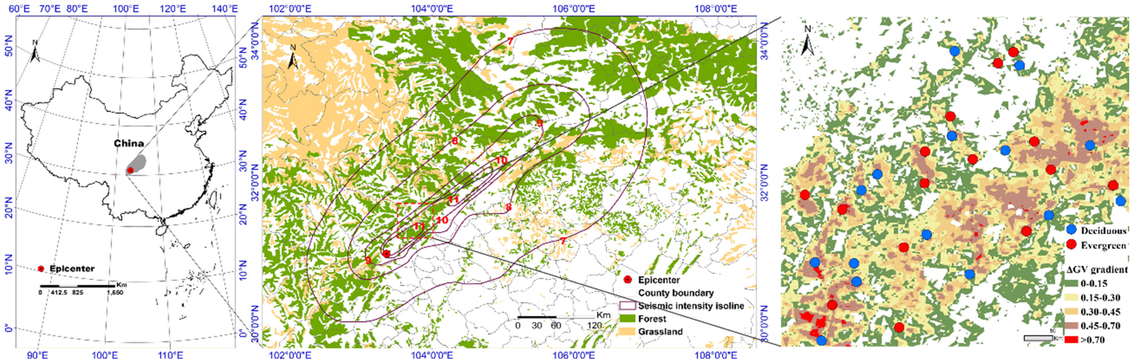
2.1. Study Area

The Wenchuan earthquake occurred on 12 May 2008, with an epicenter (31.0°N, 103.4°E) located at the southern end of the Longmenshan Thrust Fault in southwestern China (Figure 1). It ruptured over 250 km of the fault and displaced the earth’s surface up to 3 m in many places [19]. Ground shaking caused mountain collapse and landslides, which induced even more damage to the local ecosystems. With the elevation ranging from 500 to 6000 m through the impact zone, there is a clear vertical distribution of forest beginning with subtropical forests at the base and subalpine conifer forests at the top of the mountains [20]. This heavily forested area plays an important role as a carbon sink in China [21].

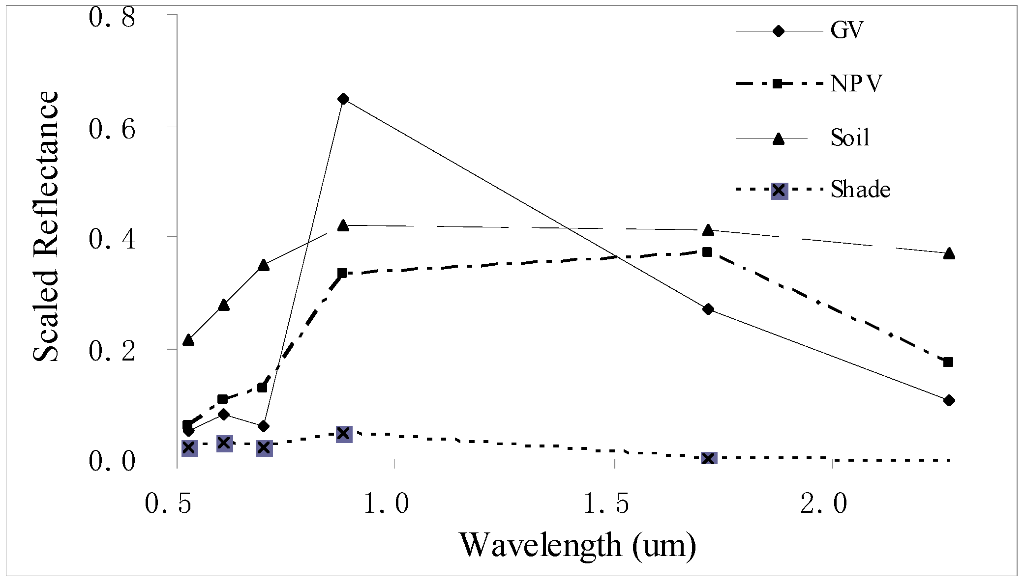
2.2. Satellite Data Analysis

Although the monitoring derived from high-resolution satellite images, such as Landsat TM or Quickbird, could be more accurate, low levels of spatial coverage and high costs limit their applications. Moreover, the weather in the Wenchuan earthquake-hit area is most cloudy, and it is almost impossible to acquire high-resolution satellite images with less than 20% cloud coverage. With higher temporal frequency, MODIS could provide images with much less cloud noise. Thus, larger coverage imagery of MODIS was used in the final estimation of forest mortality, and Landsat TM was utilized as a bridge to connect the MODIS-based mortality and field measured biomass loss. Landsat TM imagery (with spatial resolution of 30 m) from 18 September 2007 and 18 July 2008 was used to estimate forest mortality for a small typical earthquake impact area. The Landsat derived mortality map was used to guide the location of field sample plots. The mortality map, which covered the entire earthquake impacted areas, was generated from MODIS imagery. MODIS Terra images with a spatial resolution of 250 m were selected from two dates, 9 May 2007 and 24 May 2008, to represent the pre- and post-earthquake conditions, respectively.

Most of the Wenchuan earthquake-influenced areas are mountainous terrain. With the burial of disturbed trees, the newly created bare lands increased the fragmentation of the land use. Thus, most pixels in Landsat and MODIS imagery are combination of different land cover. Here, the spectral mixture analysis was applied to extract different land cover. The reflectance of each pixel is assumed to be the linear sum of the reflectance of different cover types weighted by their areal fractional presence within each pixel (Equations (1) and (2)).

$${\displaystyle \sum _{i=1}^m{\rho }_{ib}\times C_i={\rho }_b+{\epsilon }_b}$$

(1)

$${\displaystyle \sum _{i=1}^m{C}_i=1.0}$$

(2)

where m is the number of end members, ${\rho }_{ib}$ is the reflectance of pure end member i in wavelength band b (i.e., the reflectance of a pixel fully covered by end member i), C_i is the areal fraction of end member i in the focal pixel, ${\rho }_b$ is the reflectance of the entire pixel in band b, Ɛ_b is the error of fit in band b (band residual).

This work only focuses on forest ecosystem and its related biomass loss by the earthquake. A forest pixel can usually be deconvolved into 4 basic cover types or end members (Figure 2): green vegetation (GV), non-photosynthetic vegetation (NPV, i.e., dead wood), soil, and shade [22]. The reflectance of the endmembers for Landsat imagery was extracted using a technique named Sequential Maximum Angle Convex Cone (SMACC) [23], whereas pixel purity index (PPI) was applied for the endmember extraction from MODIS [24].

Although NPV can directly represent the dead wood, the difference of NPV (or NPV + soil) of pre- and post-earthquake in fact had much less correlation with the field measured biomass loss based on preliminary analysis. This might because that the damaged trees were usually buried and demonstrated little NPV signal but more bare land signal. Therefore, instead of using NPV as a proxy for dead wood as has been done in other studies [4,13], here we used the difference in green vegetation before and after the earthquake event (ΔGV) as a measure of total wood loss in each pixel. Prior to calculating ΔGV, the GV values from all the images were shade-normalized to limit the effects of topography [22].

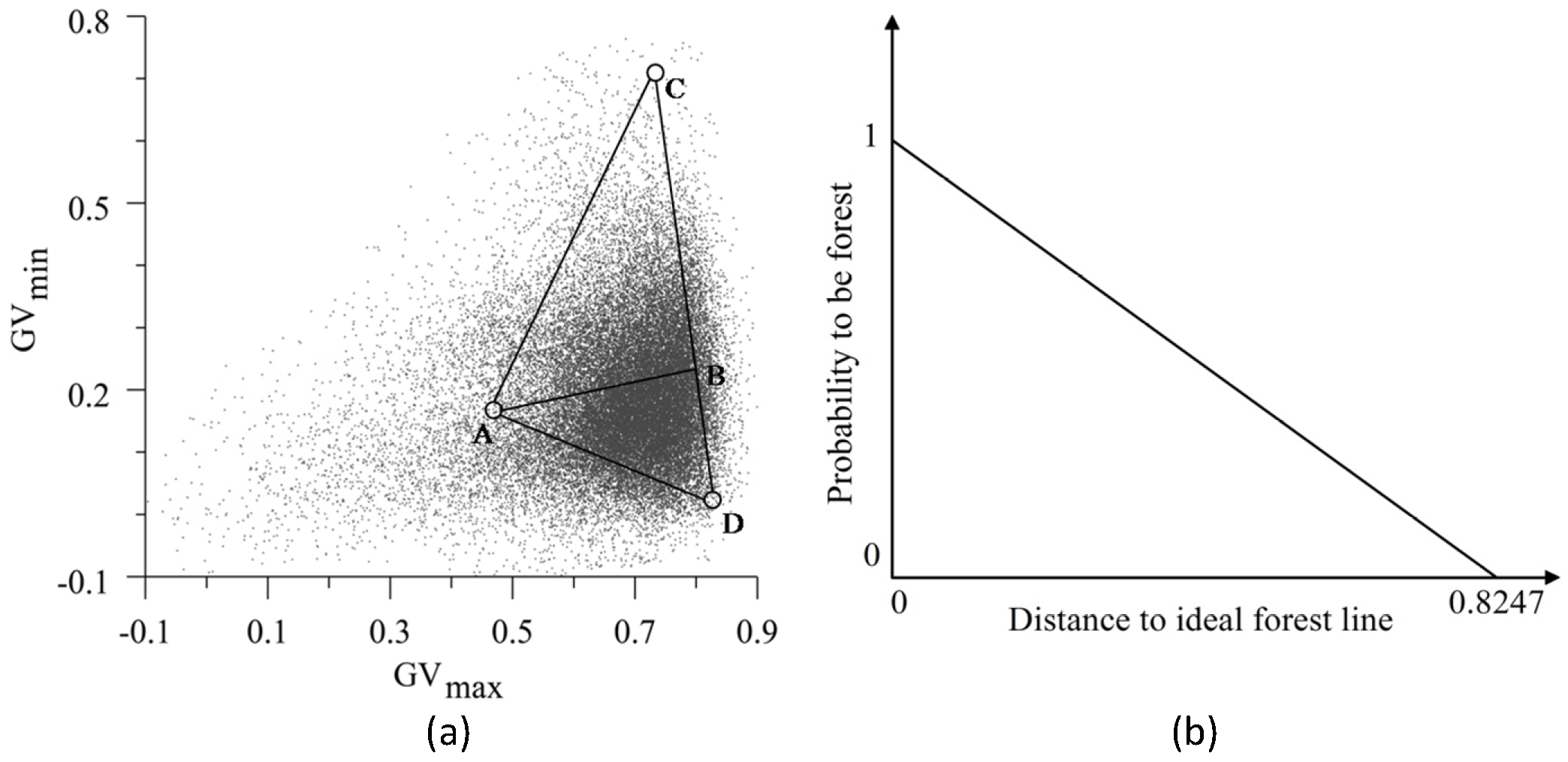
2.3. Extraction of Deciduous and Evergreen Forests

Coarse forested areas were preliminary extracted based on the land use/land cover map of China with a scale of 1/100,000 [25]. The land use map has six classes: agricultural fields, forests, grassland, water areas, urban areas, and open fields. Since part of the grassland appeared spectrally similar to forested pixels when validating on satellite images, both forests and grassland were extracted as potentially forested areas.

The potential forest areas were further classified as deciduous and evergreen based on their phenological difference, i.e., pixels with a high greenness value in the summer and a low value after senescence in the winter were classified as deciduous, while pixels that maintained a certain level of greenness throughout the year were classified as evergreen. MODIS images from January and July 2006 were used to represent the forest conditions in winter and summer, respectively. Both winter and summer images were processed by SMA, and the extracted GV values were used in forest type classification, i.e., GV from winter image represents GV_min while the GV from summer represents GV_max (Figure 3a).

The ideal points for deciduous and evergreen were set based on the vegetation map, Google images, and field investigation (Figure 3a). The pure deciduous and conifer forests were delineated preliminarily based on the vegetation map and Google images. The areas were further refined by field investigation. The distributions of the GV_min and GV_max were constructed for the selected pure deciduous and conifer pixels, and the 95th percentile values of the GV_min and GV_max were taken as the ideal points. The GV_min and GV_max for the ideal point of deciduous were set to 0.002 and 0.83, respectively, while the two values for conifer were 0.69 and 0.75. The line connecting the ideal points of deciduous (D) and evergreen (C) represented ideal forest line (Figure 3a, Equation (3))

$$ax+by+c=0$$

(3)

where x and y are axis of GV_max and GV_min in Figure 3a, respectively. The parameters a, b and c are parameters calculated by ideal points of C and D in Figure 3a (Equations (4)–(6)).

$$a=G{V}_{\min •C}-G{V}_{\min •D}$$

(4)

$$b=G{V}_{\max •D}-G{V}_{\max •C}$$

(5)

$$c=(G{V}_{\max •D}-G{V}_{\max •C})\times G{V}_{\min •C}+(G{V}_{\min •C}-G{V}_{\min •D})\times G{V}_{\max •C}$$

(6)

The likelihood that a pixel would be classified as forest was estimated by comparing its GV_min and GV_max to the forest ideal line. The points located to the right of the ideal forest line were assumed to be pure forests, whereas the points to the left were given probabilities based on their distances to the ideal line (Figure 3b, Equation (7)).

$$Dis{t}_{AB}=\frac{\left|a\times G{V}_{\max •A}+b\times G{V}_{\min •A}+c\right|}{\sqrt{a^2+b^2}}$$

(7)

The shorter the distance was, the higher probability the pixel would be classified as forest. The origin, with both GV_max and GV_min values of 0, was set as the least likelihood of 0 (Figure 3b).

After a pixel was defined to be forest, another probability was calculated to categorize it as either deciduous or evergreen by a utility function based on its distances to the two ideal points. The distances of the pixel (A) to the ideal points (C and D) were calculated (i.e., AC and AD in Figure 3a). The comparison between the distances AC and AD determined the probability of forest type classification of pixel A. The pixel was assumed to be evergreen forest with a probability of AD/(AC + AD), and deciduous with a probability of AC/(AC+AD). The shorter the distance was, the higher the probability the pixel would be classified as the related forest type.

2.4. Quantifying the Total Impacted Area

The earthquake impact boundary was estimated by comparing the ΔGV map with surface ground shaking experienced by the Wenchuan Earthquake (seismic intensity field). The seismic intensity of an earthquake is proportional to the degree of forest disturbance it causes, i.e., tree mortality declines with seismic intensity decreases. We calculated the distances of all the MODIS pixels to the Chinese seismic intensity isoline 10. The pixels located within isoline 10 (with seismic intensity > 10) were given negative distance values. The pixels were further grouped into bins based on their distances, and an average ΔGV value was calculated for each bin. It was assumed that ΔGV declined with the distance to isoline 10 until a turning point, after which ΔGV maintained a certain level regardless of the distance to isoline 10. The distance of the turning point could be the average maximum impact distance of the Wenchuan earthquake.

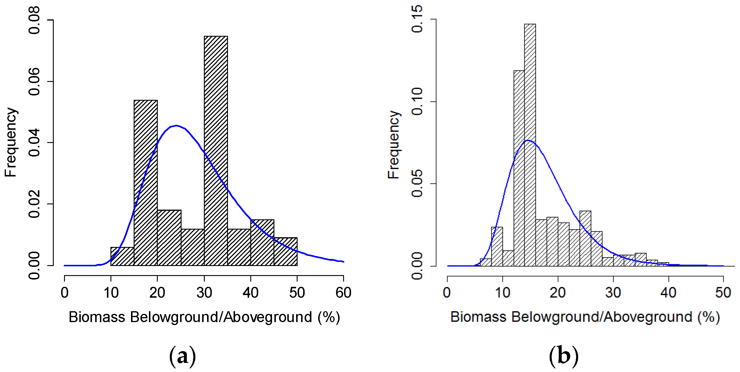
2.5. Ground-Based Tree Mortality Estimations

The ΔGV map generated by the Landsat imagery was used to guide the locations of the field sample plots and to ensure them being randomly established across the entire disturbance gradient. The full range of ΔGV was classified into five levels (<0.15, 0.15–0.3, 0.3–0.45, 0.45–0.7, and ≥0.7), and six plots were allocated in each level. Altogether, thirty forest sample plots with an area larger than 0.3 ha were established over the study area, 15 from deciduous forests and 15 from evergreen forests (Figure 1). As it is mountainous area destroyed by the Wenchuan earthquake, accessibility was also a critical criterion for selecting the plot locations. In all sample plots, most of the destroyed trees were buried or transported to the bottom of slopes, making it difficult to investigate the damage directly. Thus, the pre-earthquake conditions of each field plot were represented by three 10 m × 10 m sub-plots located in adjacent undisturbed forests. We tried to locate the sub-plots as close to the sample plots as possible, but in different directions to the plots. All subplots were less than 50 m from the damaged forest plots. Because of their proximity to the earthquake-affected field plots, the undisturbed subplots experienced similar environmental conditions to their disturbed counterpart, including elevation, slope, aspect and general forest conditions. Field surveys were conducted between July and August in both 2009 and 2010, and all trees with a diameter at breast height (DBH) ≥ 5 cm were measured with variables including tree species, DBH, tree height and tree status (living or dead).

Aboveground biomass of each tree in the field plots was calculated by published species-specific biomass allometric equations [26]. If no allometric equation existed for a particular species, the allometric equation for another species of the same the same genus (or the same family) was used. The aboveground biomass density (kg·ha⁻¹) of pre-earthquake in each sample plot was calculated based on the average biomass density of the three adjacent unaffected sub-plots. Thus, the total aboveground biomass loss of the sample plot was the product of biomass density and buried area.

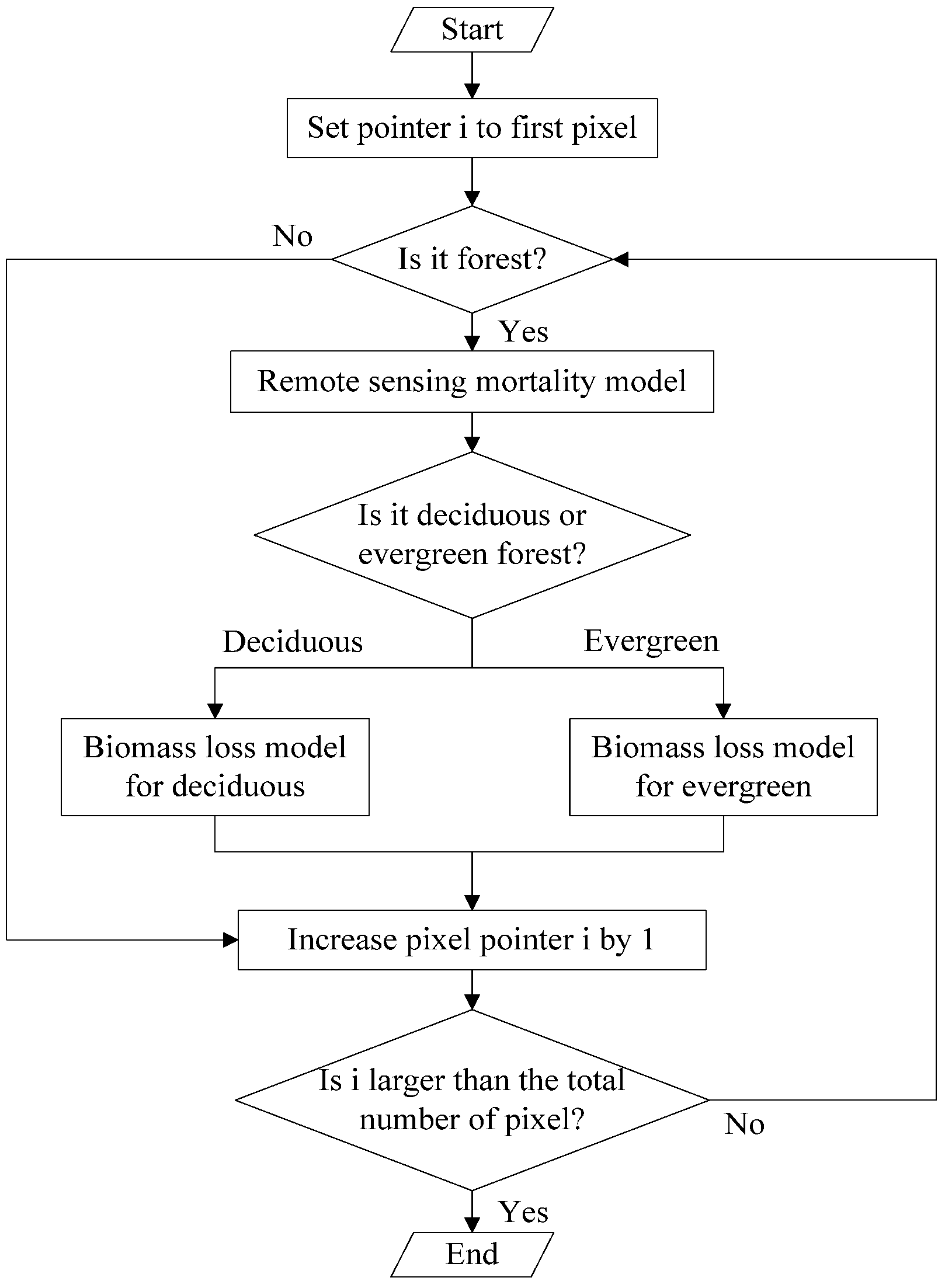
2.6. Forest Mortality Model Development

The forest biomass loss was simulated at the MODIS pixel level (250 m × 250 m), i.e., the biomass loss for each pixel was simulated separately. It included both aboveground and belowground biomass. Aboveground biomass loss was calculated by mortality models after the pixel was defined as a forest pixel. First, one mortality model was built in this work to scale the forest loss information from field measured biomass loss (kg·m⁻²) to Landsat TM (ΔGV) (Equation (8)).

$$Biolos{s}_{Above}=a\times \Delta G{V}_{Landsat}+\epsilon$$

(8)

where Bioloss_Above is the aboveground biomass loss (kg·m⁻²), a is a coefficient, and ε is the residue error, which is used in Monte Carlo simulation to estimate the uncertainty. The regression was tested by t-test and F-test in ANOVA.

Since the MODIS imagery, instead of Landsat TM, was used to estimate the total aboveground biomass loss of the entire study area following the Wenchuan earthquake, another model was built to connect the ΔGV between Landsat and MODIS satellite images (Equation (9)).

$$\Delta G{V}_{LandSat}=a_{Modis}\times \Delta G{V}_{Modis}+\epsilon$$

(9)

The mortality models were run stochastically by randomly sampling the coefficients. The sampling spaces of the coefficients in Equations (8) and (9) were defined by the parameters estimated by the regression fitting analysis.

Besides the biomass loss of aboveground, the belowground biomass loss was included in the simulation too. The belowground biomass loss was calculated as a fraction of aboveground biomass loss at plot level, since the belowground biomass was found to be in good correlation with aboveground biomass [27].

$$BioLos{s}_{Below}=r\times BioLos{s}_{Above}$$

(10)

The field measured aboveground and belowground biomass data in this work as well as previous studies [26] were used for calculating their ratio (r). Based on preliminary analysis, lognormal distribution can better simulate the ratio’s distribution in both deciduous and evergreen forests, although it is not good enough for deciduous (Figure 4). Belowground biomass loss was calculated in Monte Carlo simulation by multiplying aboveground biomass loss and the ratio of below- and aboveground biomass loss. Thus, final output from the biomass loss simulation models included both aboveground and belowground biomass.

2.7. Monte Carlo Simulation and Uncertainty Analysis

The entire process from forest type classification to forest biomass loss modeling was embedded in a Monte Carlo model (Figure 5). The boundary of the earthquake impact area and the input ΔGV of each pixel from MODIS were fixed for the input of Monte Carlo model. The boundary line of 75 km away from the seismic intensity isoline of 10 was set as the earthquake impact area. The uncertainty of the SMA when generating the ΔGV from MODIS is not included in the Monte Carlo simulation. The simulation was iterated 100 times, and the mean and variation of the biomass loss were calculated. The number of iteration in Monte Carlo was set based on the repeated trials, which output stable results, i.e., similar mean and variance values were output by different trials. In addition, the sensitivity of the simulation was examined by changing the coefficient values of forest mortality models and the GV values of ideal deciduous and evergreen points by ±20%.

As mentioned above, all pixels were simulated independently in the Monte Carlo simulation. Thus, the variance of the total biomass loss output from the Monte Carlo program would be the sum of the variance of each pixel (Equation (11)).

$$V\alpha r(T)={\displaystyle \sum _{i=1}^{N}V\alpha r(Xi)}$$

(11)

where Var(T) is the variance of total biomass loss of impact area, Var(X_i) is the variance of pixel i, and N is the total number of pixels in the impact area.

The variance in Equation (11) ignores the fact that spatial auto-correlation exists in most geographical phenomenon, i.e. closer pixels have more similar forest structure, biomass, and biomass loss. The total variance of multiple variables with correlation (Equation (12)) would be much larger than the variables without correlation (i.e., independent to each other).

$$V\alpha r(T)={\displaystyle \sum _{i=1}^{N}V\alpha r(Xi)+}2{\displaystyle \sum _{i=1}^N{\displaystyle \sum _{j=1}^M\mathrm{cov}(Xi,Xj)}}$$

(12)

where Var(Xi) is the variance of variable Xi and COV(Xi, Xj) is the covariance of variables Xi and Xj.

The covariance of any two variables is related to their Pearson correlation and standard deviation (Equation (13)).

COV(X_i, X_j) = Corr(X_i, X_j) × STD(X_i) × STD(X_j)

(13)

where corr(Xi, Xj) is the correlation between variables Xi and Xj and STD(Xi) is the standard deviation of variable Xi.

By combining Equations (12) and (13), the total variance of correlated N variables can be revised into Equation (14).

$$V\alpha r(T)={\displaystyle \sum _{i=1}^{N}V\alpha r(Xi)+}2{\displaystyle \sum _{i=1}^N{\displaystyle \sum _{j=1}^{M}corr(Xi,Xj)\times STD(Xi)\times STD（Xj)}}$$

(14)

The most popular proxy of auto-correlation, Moran’s I, is similar to Pearson correlation [28]. Equation (14) can be borrowed to calculate the biomass loss variance of all the pixels that have auto-correlation. However, it needs to be noted that not all the pixels in the earthquake impact area are correlated with each other. The spatial auto-correlation only exists within a distance (i.e., range). The pixels with distance beyond the range are independent to each other. Thus, Equation (14) need to be adjusted based on the range (Equation (15)).

$$V\alpha r(T)={\displaystyle \sum _{i=1}^{N}V\alpha r(Xi)+}2{\displaystyle \sum _{i=1}^N{\displaystyle \sum _{j=1}^M\alpha \upsilon to\_corr(X)\times STD(Xi)\times STD(Xj)}}$$

(15)

where M is the subset of the pixels that has auto-correlation with pixel i. It differs in different focal pixel i.

Since the earthquake impact area is quite large, and includes a huge number of pixels. It is extremely time consuming to calculate the 2nd part in Equation (15) by comparing every pair of pixels. We simplified Equation (15) using the standard deviation of each pixel twice instead of two pixels’ standard deviation (Equation (16)).

$${\displaystyle \sum _{j=1}^{M}STD(X_i)STD(X_j)={\displaystyle \sum _{i=1}^{M}STD(X_i)STD(X_i)}}$$

(16)

Thus, the final variance of the total biomass loss can be calculated based on Equation (17).

$$V\alpha r(T)={\displaystyle \sum _{i=1}^{N}V\alpha r(Xi)+}2{\displaystyle \sum _{i=1}^N{\displaystyle \sum _{i=1}^M\alpha \upsilon to\_corr(X)\times STD(Xi)\times STD（Xi)}}$$

(17)

where auto_corr(X) is the spatial auto-correlation Moran’s I of forest biomass loss in earthquake impact area and M is the number of pixels included in the auto-correlation range. ${\displaystyle \sum _{i=1}^{N}V\alpha r(Xi)}$ is the variance of biomass loss output by Monte Carlo simulation. Moran’s I was calculated in GIS software ArcGIS using the ΔGV map. As the study site is quite large, and ArcGIS can not calculate the Moran’s I using all the pixels. We iteratively extracted a small amount of pixels and calculated the Moran’s I value for each iteration. The averaged Moran’s I value of the 14 iterations (0.62) was used in the final calculation.

The maximum distance of the auto-correlation (range) was estimated by semivariogram in ArcGIS. Similar to the calculation of Moran’s I, we iteratively extracted a small amount of pixels to construct the semivariogram and estimated the ranges. The average range of all the 8 iterations was used to calculate the number of pixels within the range (M). The final averaged range is 6862 m with corresponding M of 2367 (i.e., number of pixels).

3. Results

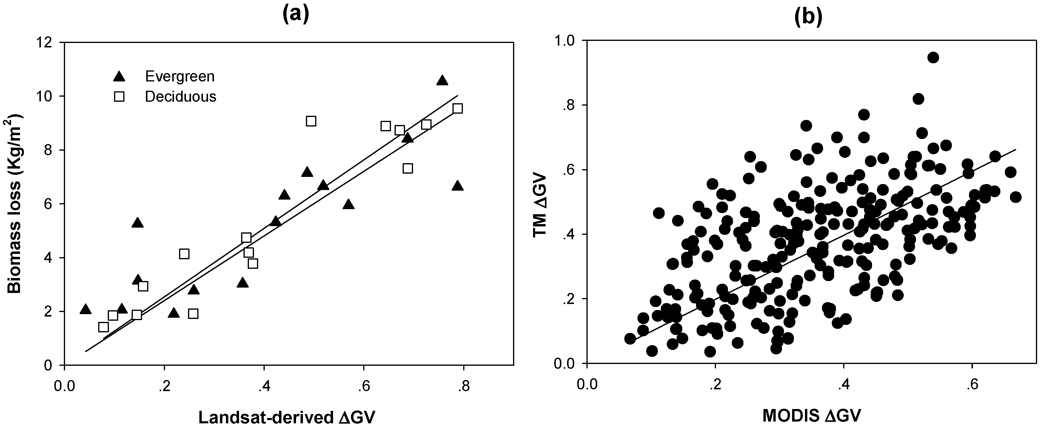
3.1. Proxy for Forest Biomass Carbon Loss

A remote sensing metric (ΔGV) validated by the field tree mortality data was used to calculate regional forest biomass loss associated with the Wenchuan earthquake. It was calculated by subtracting post-earthquake GV (2008) from pre-earthquake GV (2007). Thus, positive ΔGV values indicated net biomass loss following the Wenchuan earthquake, whereas negative ΔGV values reflected forested areas that were unaffected or had improved their green vegetation cover (growth). There was a strong and significant correlation between Landsat-derived ΔGV and the field measured biomass loss (Figure 6,

Table 1. Linear regression model and ANOVA analysis between GV from Landsat TM and field measured mortality: (a) For deciduous; (b) For evergreen; and (c) Between GV from Landsat TM and MODIS.

			Estimated (B)	Standard Error	t-Value	Pr (>|t|)		Df	Sum of Square	Mean of Square	F Value	Pr (>F)
(a)	Deciduous	TM_ΔGV (900 m2)	12,737.9	604.1	21.09	<0.0001	TM_ΔGV	1	537,853,472	537,853,472	444.65	<0.0001
							Residuals	14	13,343,914	1,213,083
(b)	Evergreen	TM_ΔGV (900 m2)	11,979.8	858.3	13.96	<0.0001	TM_ΔGV	1	457,454,043	457,454,043	194.81	<0.0001
							Residuals	14	32,875,103	2,348,222
(c)		MODIS_ΔGV	0.99171	0.02504	39.61	<0.0001	MODIS_ΔGV	1	36.601	36.601	1568.8	<0.0001
							Residuals	249	5.809	0.023

The unit is kg/900 m², corresponding to the pixel size of Landsat.

). Thus, ΔGV was used as a proxy for forest biomass loss resulting from the Wenchuan earthquake. As the regression models have intercept of 0 and the R² is invalid, the t-test and F-test were applied to evaluate the significance of the regression (Table 1).

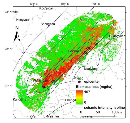
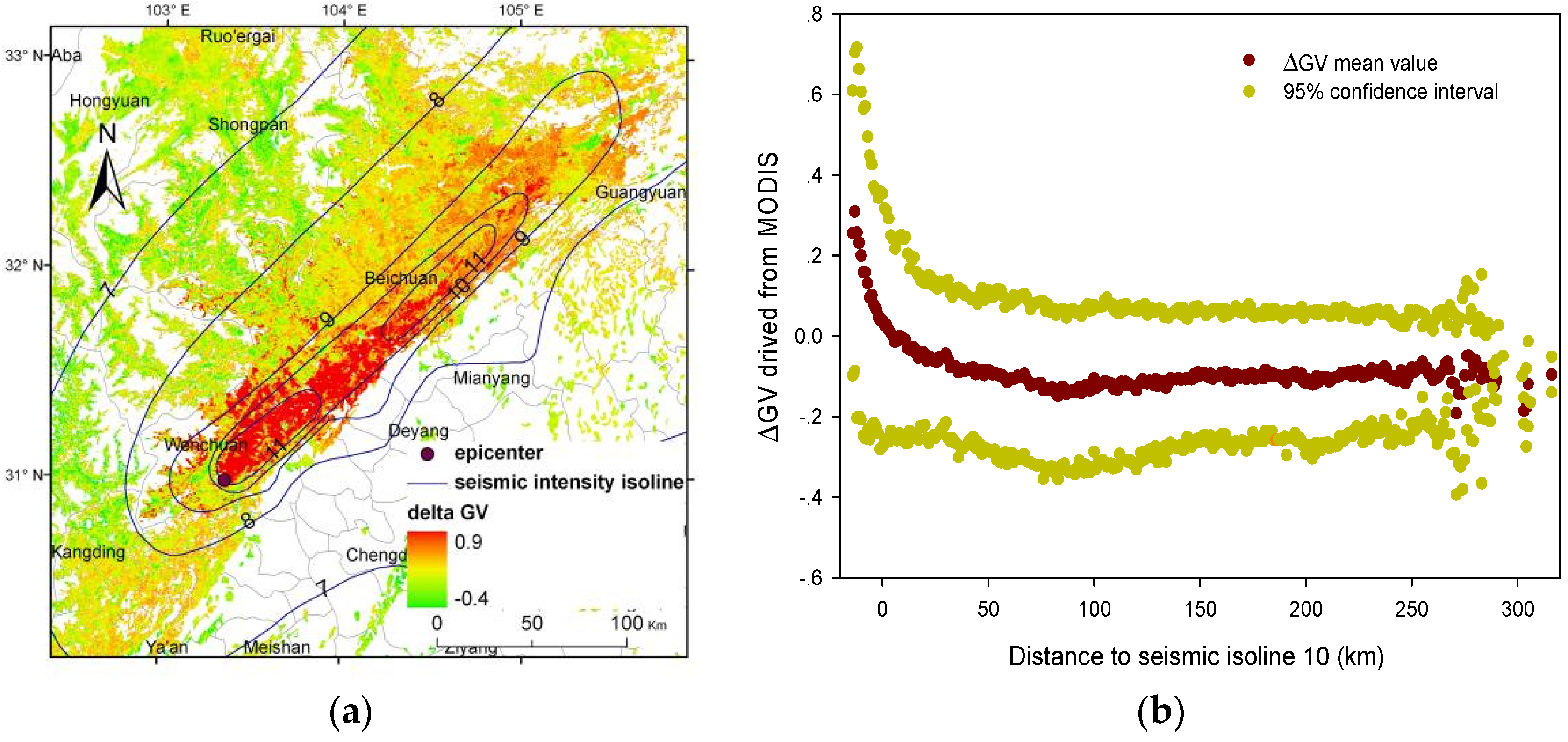
3.2. Spatial Pattern of Forest Mortality

The severity of forest mortality was consistent with the seismic intensity of the Wenchuan earthquake. The earthquake had a strong effect on tree mortality at the fault zone (Figure 7a). Field investigation found the most intensive biomass losses, including both above and belowground loss, were 133 Mg·ha⁻¹ in the evergreen sites and 125 Mg·ha⁻¹ in the deciduous sites. The highest biomass loss based on the ΔGV map was 167 Mg·ha⁻¹. The influence of the earthquake declined rapidly with distance away from the fault trace (Figure 7a), especially within regions of seismic intensity > 9 (Figure 7). The average biomass loss was estimated to be as high as 5.4 Mg·ha⁻¹ at the fault zone (with a corresponding ΔGV of 0.3), and it decreased rapidly on a slope of 0.25 Mg·km⁻¹ with distance away from the fault line (Figure 7b).

Forest mortality (i.e., ΔGV) continued to decrease up to a distance of 75 km away from seismic intensity isoline 10 (Figure 7b), after which ΔGV values remained stable. The turning point, i.e., 75 km away from seismic isoline 10, was therefore set as the average maximum distance (boundary) for forests affected by the Wenchuan earthquake. The forests within this boundary were further evaluated for their biomass loss following the Wenchuan earthquake.

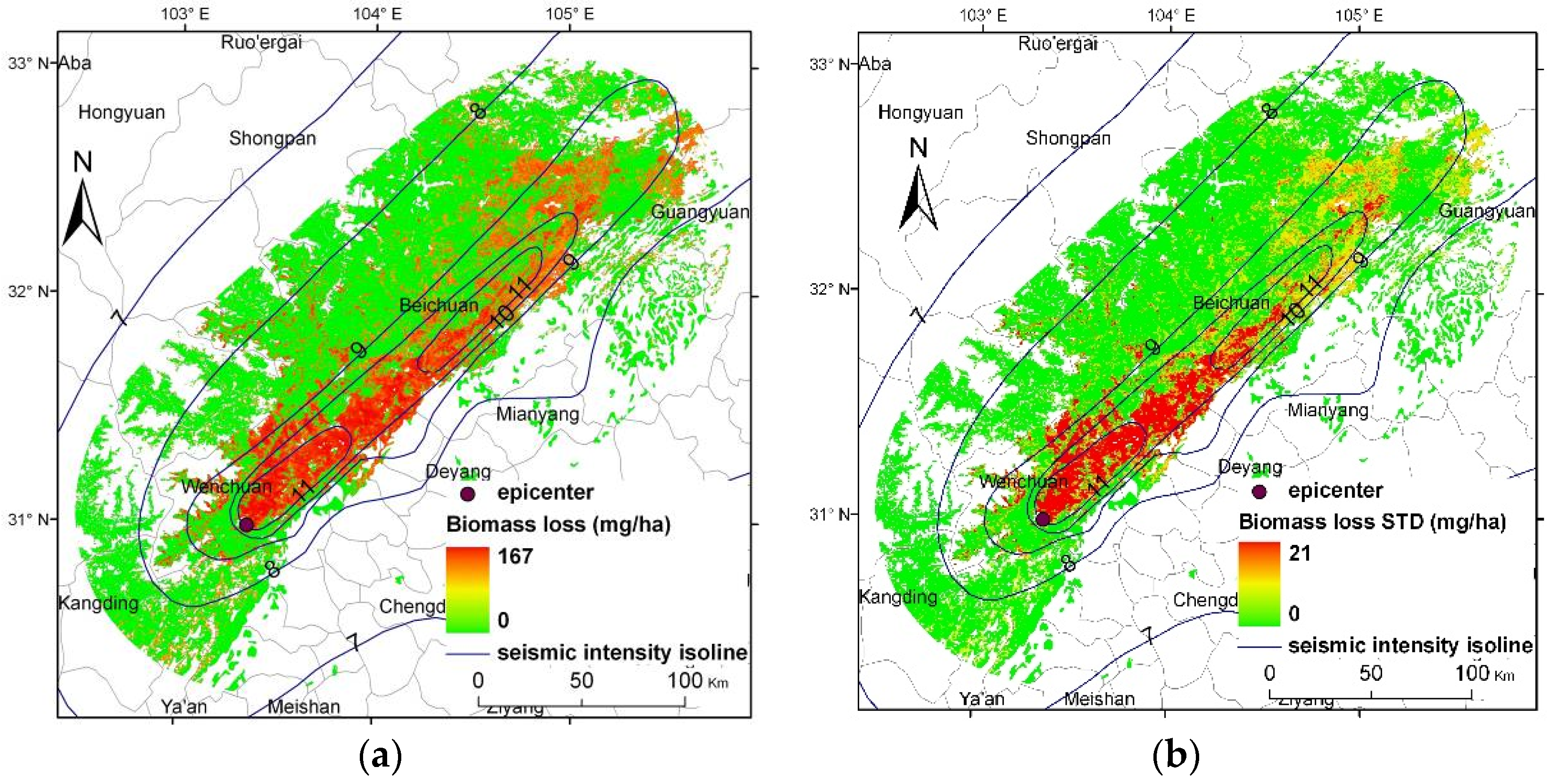
3.3. Quantification of Forest Biomass Loss

The Wenchuan earthquake has induced significant forest biomass loss in a relatively small impact area. Nearly 32,244 km² of forests are located within the Wenchuan earthquake impact zone (Figure 8). About 10,757 km² of forest area (33.4% of the total forest area within the study area) showed biomass loss due to the earthquake.

The forests had a significant biomass loss of 21.8 Tg (with equivalent carbon loss of 10.9 Tg∙C), including aboveground and belowground biomass. The 95% confidence interval of the biomass loss was 20.8–22.8 Tg. In addition, since deciduous forests dominate the landscape of this region, most of the damage occurred in these forests. About 8677 km² of deciduous forests were affected and resulted in a total biomass loss of 17.9 Tg (equivalent to 8.95 Tg∙C). Only 2079 km² of evergreen forests were affected with a corresponding biomass loss of 3.9 Tg (1.95 Tg∙C).

The variation of coefficient values in the mortality models explained the largest variation in total forest loss estimates (

Table 2. The sensitivity analysis of the simulation: the biomass loss (Tg) output by changing the value of coefficients and parameters in ±20%.

Items	Nominal Value	+20%	−20%
Coefficient of deciduous mortality model (aLandsat_d)	14.2
Coefficient of evergreen mortality model (aLandsat_e)	13.3	26.1	17.4
Coefficient of scale model between MODIS and Landsat (aModis)	0.99	26.2	17.4
Ideal points’ GVmin (deciduous)	0.002
Ideal points’ GVmin (evergreen)	0.69	22.0	21.5
Ideal points’ GVmax (deciduous)	0.83
Ideal points’ GVmax (evergreen)	0.75	21.4	21.9
Maximum forest distance (dfor)	0.8247	21.8	21.7

). On the other hand, forest classification had little effect on the uncertainty of the simulation, i.e., the parameter values of ideal points of deciduous and evergreen trees had relatively little influence on the variation of total carbon loss. The changes to the ideal points of forest type did not significantly change the forest likelihood probability for most pixels.

3.4. Factors Influencing Forest Damage Patterns

In addition to seismic intensity of the earthquake, topography and tree characteristics also played important roles in forest mortality (Figure 9). Forests located on steeper slopes sustained higher rates of mortality (Figure 9a), i.e., a Pearson correlation coefficient of 0.66 was found between topographic slope and ΔGV (p-value < 0.001).

Furthermore, ΔGV was found to be well correlated with tree size based on field survey (Figure 9b,c). It had Pearson correlation coefficients of 0.42 and 0.46 with tree’s DBH and height, respectively, and both had p-values < 0.01 (Figure 9b,c). The larger trees sustained more damages from the earthquake. In general, topographical conditions played a more significant role in earthquake-induced tree mortality than individual tree characteristics. The dominant species in the study area, such as Alnus cremastogyne, Cunninghamia lanceolata, Cryptomeria fortuner and Betula utilis, also had the highest mortality rates.

4. Discussion

4.1. Improvement of the Synthetic Approach in Earthquake Influence Assessment

There are a few studies that explicitly evaluated the impacts of Wenchuan earthquake on forests at the regional scale [15,16,17]. However, large uncertainties exist in these studies, mainly due to the lack of appropriate methodology and field data. To our knowledge, this is the first study to provide ground-based evidence that Wenchuan earthquakes impact forest mortality.

Instead of using political jurisdiction boundary like in other Wenchuan earthquake related research [15,16,17], this study used seismic intensity field to define the earthquake impact zone. Forest impacted zone was defined by a boundary that extended 75 km beyond the seismic intensity 10 isoline. This outline is consistent with the spatial pattern of landslides triggered by the Wenchuan earthquake, which declined with distance away from the epicenter until about 80 km from the surface rupture [29]. The new Wenchuan impact boundary outlined in this study greatly improved the accuracy of the earthquake impact assessment compared with previous studies that used jurisdiction boundaries alone [15,16,17]. Using jurisdiction boundary can significantly deviate the estimation of the earthquake effects. For example, Jiang et al. [17] evaluated the Wenchuan earthquake-damaged forest area as 1599 km², while our approach estimated an impact area of 10,757 km².

The differences in methodology may lead to different forest mortality results. For example, Chen et al. estimated 20.7% forest destroyed by Wenchuan earthquake using InSAR tools [16]; Jiang et al. found only 13.8% of forests was affected according to a quantified threshold based on MODIS NDVI data [17]. In this study, we suggested the fraction of impacted forest areas was 33.4%, which was in good agreement with our field experience.

Our estimation of the total forest biomass loss that resulted from the Wenchuan earthquake (10.9 Tg in carbon) was much smaller than previously reported (235 Tg∙C) [15]. The main cause for the difference stems from the differences in the methodologies used. Ren et al. [15] used an administrative boundary to quantify the impact zone, which obviously overestimated the influence of this earthquake by including tree mortality induced by other disturbances. In addition, Ren et al. [15] did not include any field measured mortality data to calibrate their model simulations, which may have significantly biased their estimates. By adding detailed field investigation and a precisely quantified impact zone, our approach is able to obtain a more accurate estimate of forest biomass loss.

Overall, two important characteristics of the Wenchuan earthquake impact were observed. First, the earthquake had a strong effect within the fault zone, where extremely high mortality was observed. The aboveground biomass loss (117 Mg·ha⁻¹) in the Wenchuan fault zone was even higher than the biomass loss following hurricane Katrina (87 Mg·ha⁻¹) [30]. Second, the influence of the earthquake declined rapidly with distance away from the fault zone, suggesting the entire impact area was relatively small when compared with other disturbances [4].

4.2. Factors Impacting Tree Mortality Following Earthquake Events

The damage to a tree is a result of multiple factors including tree and stand characteristics and environmental conditions. The prime impact factor on earthquake-induced tree mortality is topography. Trees located on hills with steep slopes experienced higher mortality rates (Figure 9a). This is consistent with the findings in other earthquake-related studies [31,32] as well as the field investigation in our work, i.e., the landslides and mountain collapses were more often found in topographically steep regions and consequently buried more trees. Precipitation may also be critical to tree mortality, as heavy raining may trigger more landslide and debris flow. Unfortunately, there is no proper climate data available and no related analysis could be carried out.

More middle-sized trees were damaged in Wenchuan earthquake, although old trees are more susceptible (Figure 9). This is because most forests in the Wenchuan earthquake area had middle-sized trees. Moreover, there was no significant difference in tree mortality between tree species. The species with higher mortality were also the dominant species in this area. The lack of correlation between tree species and vulnerability is unique to earthquake disturbance, as most other forms of natural disturbance, e.g., wind [33], fire [34], drought [35] and insect attack [6], are closely linked to tree species.

4.3. Earthquakes Act as Major Carbon Dynamic Drivers

Our results showed that earthquakes might act as major drivers of forest carbon dynamics, especially in tectonically active regions. The trees buried during earthquake usually have low turnover rates with long life span (decades to centuries). Without the carbon pools of these buried woody mass, the carbon stock estimation would be biased and the regional carbon dynamics would be misinterpreted [36]. It was reported that Chinese forests had a living biomass carbon stock of 4.75 Pg C in 1998 [37]. The biomass carbon loss associated with the Wenchuan earthquake offset the biomass carbon in Chinese forests by 0.23%. On average, 14.7 earthquakes of magnitude > 5.75 occur every month at shallow depth (<70 km) around the world [38]. In China, 16.3 earthquakes with magnitude 5.0 or greater occur each year [39]. As earthquakes continue to occur at this frequency or higher, more forests will likely be exposed to this form of disturbance, particularly in tectonically active regions. Our results indicate that earthquake-induced biomass carbon loss comprises a more important component of the carbon budget than previously expected. Thus, the disturbance of the earthquake and the dynamics of the buried woody mass need to be included in the evaluation of regional carbon balance. Despite their importance, the earthquake-induced carbon pool has largely been missed and is not currently represented in the calculations of carbon budget.

4.4. Uncertainties and Limitations of the Synthesis Approach

Uncertainties in our approach are mainly attributed to the definition of the areal impact boundary by the earthquake, the performance of the SMA to produce ΔGV, and the coefficient values of the forest mortality models. Our robust field measurements significantly improved the mortality models, help set the ideal endmembers, and therefore provide more precise predictions of earthquake impacts. Although the field survey was well designed and its sampling sites were allocated across the entire damaged gradient, uncertainties still exist in the inventory data, mainly coming from measurement errors and sampling errors. For example, we only record the trees with DBH greater than 5 cm and likely underestimate the damage that occurred in small trees. On the other hand, the selection of ideal points of forest types had relatively little effect on the estimation of forest loss (Table 2). This is mainly due to the fact that most non-forest areas were excluded in the final calculation based on land use maps. Extra caution is needed if non-forest areas are included in the analysis, which may increase the uncertainty regarding the biomass loss estimate. Another additional limitation of our study is the difficulty of investigating the earthquake-induced forest damage directly. Since trees are usually buried following earthquake events, pre-earthquake forest conditions were approximated by measuring the adjacent undisturbed forest.

The Monte Carlo program output relatively small variation of the biomass loss (with standard deviation coefficient of 3%). One reason is that some of the input information was set as deterministic due to the complication of the process, including the boundary of impact area and ΔGV extracted from SMA. Another important reason is the independence of the pixels. Although there is spatial auto-correlation in biomass loss, the range of the auto-correlation (2367 pixels) is relatively small compare to the impact area (172,113 pixels). One pixel is only auto-correlated to less than 2% of the total pixels of the impact areas. This is mainly because the study area is a mountainous area with steep valleys. The land use and vegetation are fragmented. This is significantly different from plains. The Monte Carlo simulations have the limitation to improve the biomass loss estimation at any specific location (pixel), which was proven by Healey et al. [40]. However, biomass loss at landscape level can be fully accredited due to the independence among pixels, which decreases the uncertainty of estimation.

5. Conclusions

Earthquakes have unexpected and tragic effects on ecological systems. The synthetic approach developed in this work could efficiently quantify the forest biomass carbon loss following an earthquake event. Our results reveal that the Wenchuan earthquake had a strong and measurable impact on tree mortality with a total biomass carbon loss of 10.9 Tg∙C. However, the damages were highly localized resulting in a smaller impact area than previously considered. As such, the earthquake-induced dead trees represent a large forest carbon pool that is not yet fully recognized in forest carbon accounting. Failing to account for the effects of earthquake disturbance may bias carbon stock estimation and misinterpret carbon dynamics.

References

1. Garwood, N.C.; Janos, D.P.; Brokaw, N. Earthquake caused landslides: A major disturbance to tropical forests. Science 1979, 205, 997–999. [Google Scholar] [CrossRef] [PubMed]
2. Gorum, T.; Fan, X.; Westen, C.J.; Huang, R.; Xu, Q.; Tang, C.; Wang, G. Distribution pattern of earthquake-induced landslides triggered by the 12 May 2008 Wenchuan earthquake. Geomorphology 2011, 133, 152–167. [Google Scholar] [CrossRef]
3. Allen, R.B.; Bellingham, P.J.; Wiser, S.K. Immediate damage by an earthquake to a temperate montane forest. Ecology 1999, 80, 708–714. [Google Scholar] [CrossRef]
4. Chambers, J.Q.; Fisher, J.I.; Zeng, H.C.; Chapman, E.L.; Baker, D.B.; Hurtt, G.C. Hurricane Katrina’s carbon footprint on U.S. gulf coast forests. Science 2007, 318, 1107. [Google Scholar] [CrossRef] [PubMed]
5. Saleska, R.D.; Didan, K.; Huete, A.R.; Da Rocha, H.R. Amazon forests green-up during 2005 drought. Science 2007, 318, 612. [Google Scholar] [CrossRef] [PubMed]
6. Kurz, W.A.; Dymond, C.C.; Stinson, G.; Rampley, G.J.; Neilson, E.T.; Carroll, A.L.; Ebata, T.; Safranyik, L. Mountain pine beetle and forest carbon feedback to climate change. Nature 2008, 452, 987–990. [Google Scholar] [CrossRef] [PubMed]
7. Parsons, T.; Geist, E.L. The 2010–2014. 3 global earthquake rate increase. Geophys. Res. Lett. 2014, 41, 4479–4485. [Google Scholar]
8. Webecs Consultants LTD. Earthquakes—What Are the Long Term Trends? Available online: http://www.earth.webecs.co.uk/ (assessed on 19 May 2015).
9. Körner, C. Slow in, rapid out—Carbon flux studies and Kyoto targets. Science 2003, 300, 1242–1243. [Google Scholar] [CrossRef] [PubMed]
10. Pascal, V.; Glenn, S.H.; Richard, D.P. Earthquake impacts in old-growth Nothofagus forests in New Zealand. J. Veg. Sci. 2001, 12, 417–426. [Google Scholar]
11. Asner, G.P.; Anderson, C.B.; Martin, R.E.; Knapp, D.E.; Tupayachi, R.; Sinca, F.; Malhi, Y. Landscape-scale changes in forest structure and functional traits along an Andes-to-Amazon elevation gradient. Biogeosciences 2014, 11, 843–856. [Google Scholar] [CrossRef]
12. Asner, G.P.; Hicke, J.A.; Lobell, D.B. Per-pixel analysis of forest structure: Vegetation indices, spectral mixture analysis and canopy reflectance modeling. In Methods and Applications for Remote Sensing of Forests: Concepts and Case Studies; Wulder, M., Franklin, S.E., Eds.; Kluwer Academic Publishers: New York, NY, USA, 2003. [Google Scholar]
13. Negrón-Juárez, R.; Baker, D.B.; Chambers, J.Q.; Hurttd, G.C.; Goosem, S. Multi-scale sensitivity of Landsat and MODIS to forest disturbance associated with tropical cyclones. Remote Sens. Environ. 2014, 140, 679–689. [Google Scholar] [CrossRef]
14. Huang, R.Q.; Fan, X.M. The landslide story. Nat. Geosci. 2013, 6, 325–326. [Google Scholar] [CrossRef]
15. Ren, D.; Wang, J.; Fu, R.; Karoly, D.J.; Hong, Y.; Leslie, L.M.; Fu, C.; Huang, G. Mudslide-caused ecosystem degradation following Wenchuan earthquake 2008. Geophys. Res. Lett. 2009, 36, L05401. [Google Scholar] [CrossRef]
16. Chen, F.L.; Guo, H.D.; Ishwaran, N.; Zhou, W.; Yang, R. X.; Jing, L.H.; Chen, F.; Zeng, H.C. Synthetic aperture radar (SAR) interferometry for assessing Wenchuan earthquake (2008) deforestation in the Sichuan Giant Panda Site. Remote Sens. 2014, 6, 6283–6299. [Google Scholar] [CrossRef]
17. Jiang, W.G.; Jia, K.; Wu, J.J.; Tang, Z.H.; Wang, W.J.; Liu, X.F. Evaluating the vegetation recovery in the damage area of Wenchuan earthquake using MODIS data. Remote Sens. 2015, 7, 8757–8778. [Google Scholar] [CrossRef]
18. Stone, R.A. Deeply scarred land. Science 2009, 324, 713–714. [Google Scholar] [CrossRef] [PubMed]
19. Zhang, W.; Lin, J.; Peng, J.; Lu, Q. Estimating Wenchuan earthquake induced landslides based on remote sensing. Int. J. Remote Sens. 2010, 31, 3495–3508. [Google Scholar] [CrossRef]
20. Lu, T.; Ma, K.; Zhang, W.; Fu, B. Differential responses of shrubs and herbs present at the Upper Minjiang River basin (Tibetan Plateau) to several soil variables. J. Arid Environ. 2006, 67, 373–390. [Google Scholar] [CrossRef]
21. Fang, J.Y.; Kato, T.C.; Guo, Z.D.; Yang, Y.H.; Hu, H.F.; Shen, H.H.; Zhao, X.; Kishimoto-Mo, A.W.; Tang, Y.H.; Houghton, R.A. Evidence for environmentally enhanced forest growth. Proc. Natl. Acad. Sci. USA 2014, 111, 9527–9532. [Google Scholar] [CrossRef] [PubMed]
22. Souza, C.M., Jr.; Roberts, D.A.; Cochrane, M.A. Combing spectral and spatial information to map canopy damage from selective logging and forest fires. Remote Sens. Environ. 2005, 98, 329–343. [Google Scholar] [CrossRef]
23. Gruninger, J.H.; Ratkowski, A.J.; Hoke, M.L. The sequential maximum angle convex cone (SMACC) endmember model. In Proceedings of the SPIE Algorithms and Technologies for Multispectral, Hyperspectral, and Ultraspectral Imagery X, Orlando, FL, USA; 2004; Volume 5425, pp. 1–14. [Google Scholar]
24. Boardmann, J.; Kruse, F.A.; Green, R.O. Mapping target signatures via partial unmixing of AVIRIS data. In Proceeding of the Summaries of the Fifth Annual JPL Airborne Earth Science Workshop, Pasadena, CA, USA, 23 January 1995; Volume 1, pp. 23–26.
25. Liu, J.Y.; Liu, M.L.; Deng, X.Z.; Zhuang, D.F.; Zhang, Z.X.; Luo, D. The land use and land cover change database and its relative studies in China. J. Geogr. Sci. 2002, 12, 275–282. [Google Scholar]
26. Luo, T.; Li, W.; Zhu, H. Estimated biomass and productivity of natural vegetation on the Tibetan Plateau. Ecol. Appl. 2002, 12, 980–997. [Google Scholar] [CrossRef]
27. Li, Z.; Kurz, W.A.; Apps, M.J.; Beukema, S.J. Belowground biomass dynamics in the carbon budget model of the Canadian forest sector: Recent improvements and implications for the estimation of NPP and NEP. Can. J. For. Res. 2003, 33, 126–136. [Google Scholar] [CrossRef]
28. Moran, P.A.P. Notes on continuous stochastic phenomena. Biometrika 1950, 37, 17–23. [Google Scholar] [CrossRef] [PubMed]
29. Dai, F.C.; Xu, C.; Yao, X.; Xu, L.; Tu, X.B.; Gong, Q.M. Spatial distribution of landslides triggered by the 2008 Ms 8.0 Wenchuan earthquake, China. J. Asian Earth Sci. 2011, 40, 883–895. [Google Scholar] [CrossRef]
30. Chapman, E.L.; Chambers, J.Q.; Ribbeck, K.F.; Baker, D.B.; Tobler, M.A.; Zeng, H.C.; White, D.A. Hurricane Katrina impacts on forest trees of Louisiana’s Pearl River basin. For. Ecol. Manag. 2008, 256, 883–889. [Google Scholar] [CrossRef]
31. Lin, W.T.; Chou, W.C.; Lin, C.Y.; Huang, P.H.; Tsai, J.S. Vegetation recovery monitoring and assessment at landslides caused by earthquake in Central Taiwan. For. Ecol. Manag. 2005, 210, 55–66. [Google Scholar] [CrossRef]
32. Lu, T.; Zeng, H.C.; Luo, Y.; Wang, Q.; Shi, F.S.; Sun, G.; Wu, Y.; Wu, N. Monitoring vegetation recovery after China’s May 2008 Wenchuan earthquake using Landsat TM time-series data: A case study in Mao County. Ecol. Res. 2012, 27, 955–966. [Google Scholar] [CrossRef]
33. Usbeck, T.; Wohlgemuth, T.; Dobbertin, M.; Pfister, C.; Bürgi, A.; Rebetez, M. Increasing storm damage to forests in Switzerland from 1858 to 2007. Agric. For. Meteorol. 2010, 150, 47–55. [Google Scholar] [CrossRef]
34. Kelly, R.; Chipman, M.L.; Higuera, P.E.; Stefanova, I.; Brubaker, L.B.; Hu, F.S. Recent burning of boreal forests exceeds fire regime limits of the past 10,000 years. Proc. Natl. Acad. Sci. USA 2013, 110, 13055–13060. [Google Scholar] [CrossRef] [PubMed]
35. Ma, Z.; Peng, C.; Zhu, Q.; Chen, H.; Yu, G.; Li, W.; Zhou, X.; Wang, W.; Zhang, W. Regional drought-induced reduction in the biomass carbon sink of Canada’s boreal forests. Proc. Natl. Acad. Sci. USA 2012, 109, 2423–2427. [Google Scholar] [CrossRef] [PubMed]
36. Moroni, M.T.; Morris, D.M.; Shaw, C.; Stokland, J.N.; Harmon, M.E.; Fenton, N.J.; Merganicˇova, K.; Merganic, J.; Okabe, K.; Hagemann, U. Buried wood: A common yet poorly documented form of deadwood. Ecosystems 2015, 18, 605–628. [Google Scholar] [CrossRef]
37. Fang, J.Y.; Chen, A.P.; Peng, C.H.; Zhao, S.Q.; Ci, L.J. Changes in forest biomass carbon storage in China between 1949 and 1998. Science 2001, 292, 2320–2322. [Google Scholar] [CrossRef] [PubMed]
38. Main, I.G.; Li, L.; McCloskey, J.; Naylor, M. Effect of the Sumatran mega-earthquake on the global magnitude cut-off and event rate. Nat. Geosci. 2008, 1, 142. [Google Scholar] [CrossRef]
39. Qu, Y.; Wang, H.; Wu, C.; Feng, J.; Chen, Y.; Li, Y.; Wang, X. Analysis on statistic characteristics of seismic gap in Chinese mainland. Acta Seismol. Sin. 2010, 32, 544–556. [Google Scholar]
40. Healey, S.P.; Urbanski, S.P.; Patterson, P.L.; Garrard, C. A framework for simulating map error in ecosystem models. Remote Sens. Environ. 2014, 150, 207–217. [Google Scholar] [CrossRef]
Figure 1. The location of Wenchuan earthquake and field sample plots.
Remotesensing 08 00252 g001
Figure 2. The typical spectral reflectance of the four endmembers used in Spectral Mixture Analysis.
Remotesensing 08 00252 g002
Figure 3. The scatter plots of fraction of green vegetation (GV) in summer and winter (a) and the forest utility function (b). Points C and D represent ideal evergreen and deciduous forests, respectively; line CD represents the ideal forest line. AC and AD represent relative probabilities for a pixel to contain evergreen or deciduous forest. A pixel is assumed to be evergreen forest with a probability of AD/(AC + AD), and deciduous with a probability of AC/(AC + AD).
Remotesensing 08 00252 g003
Figure 4. The distribution of biomass ratio between belowground and aboveground: (a) deciduous with log-mean of 3.3 and log-STD 0.3; and (b) evergreen with log-mean of 2.8 and log-STD 0.3.
Remotesensing 08 00252 g004
Figure 5. The Monte Carlo simulation routine for estimating biomass loss.
Remotesensing 08 00252 g005
Figure 6. The relationship between field measured forest biomass loss rate and: Landsat TM ΔGV (a); and Landsat TM and MODIS ΔGV (b).
Remotesensing 08 00252 g006
Figure 7. MODIS-derived ΔGV (a); and the relationship between MODIS-derived ΔGV and distance away from Seismic Intensity Isoline 10 (b). Positive ΔGV represents forest loss, whereas negative indicates intact or improved forest conditions. A negative distance in (b) indicates pixels that were located within the seismic intensity isoline, i.e., the seismic intensity of these pixels was greater than 10.
Remotesensing 08 00252 g007
Figure 8. Mean value (a) and variance value (b) of forest biomass loss from the Wenchuan earthquake at the pixel scale.
Remotesensing 08 00252 g008
Figure 9. The relationship between ΔGV and terrain slope (a); tree’s diameter at breast height (b); and tree’s height (c). The brown and green points represent deciduous and evergreen forests, respectively.
Remotesensing 08 00252 g009