Article

An Automatic Building Extraction and Regularisation Technique Using LiDAR Point Cloud Data and Orthoimage †

1
Faculty of Information Technology, Monash University, Clayton VIC 3800, Australia
2
School of Information and Communication Technology Griffith Sciences, Griffith University, Nathan QLD 4111, Australia
3
School of Engineering and Information Technology, Federation University Australia, Churchill VIC 3842, Australia
*
Author to whom correspondence should be addressed.
This paper is an extended version of our paper Fusion of LiDAR data and multispectral imagery for effective building detection based on graph and connected component analysis, published in The International Archives of Photogrammetry, Remote Sensing and Spatial Information Sciences.
Submission received: 6 December 2015 / Revised: 2 February 2016 / Accepted: 1 March 2016 / Published: 17 March 2016

Abstract

:
The development of robust and accurate methods for automatic building detection and regularisation using multisource data continues to be a challenge due to point cloud sparsity, high spectral variability, urban objects differences, surrounding complexity, and data misalignment. To address these challenges, constraints on object’s size, height, area, and orientation are generally benefited which adversely affect the detection performance. Often the buildings either small in size, under shadows or partly occluded are ousted during elimination of superfluous objects. To overcome the limitations, a methodology is developed to extract and regularise the buildings using features from point cloud and orthoimagery. The building delineation process is carried out by identifying the candidate building regions and segmenting them into grids. Vegetation elimination, building detection and extraction of their partially occluded parts are achieved by synthesising the point cloud and image data. Finally, the detected buildings are regularised by exploiting the image lines in the building regularisation process. Detection and regularisation processes have been evaluated using the ISPRS benchmark and four Australian data sets which differ in point density (1 to 29 points/m 2 ), building sizes, shadows, terrain, and vegetation. Results indicate that there is 83% to 93% per-area completeness with the correctness of above 95%, demonstrating the robustness of the approach. The absence of over- and many-to-many segmentation errors in the ISPRS data set indicate that the technique has higher per-object accuracy. While compared with six existing similar methods, the proposed detection and regularisation approach performs significantly better on more complex data sets (Australian) in contrast to the ISPRS benchmark, where it does better or equal to the counterparts.

Graphical Abstract

1. Introduction

The automated extraction and localisation of urban objects is an active field of research in photogrammetry with the focus on detailed representations. Building being a key urban object is indispensable to diverse applications in cartographic mapping, urban planning, civilian and military emergency responses, and the crisis management [1,2]. Accurate and updated information of the buildings is quite imperative to keep these applications operational. At a first glance, a building may appear to be a simple object that can be easily classified and extracted. However, in reality, automatic building extraction is quite challenging due to the differences in viewpoint, surrounding environment, and complex shape and size of the buildings. There have been several attempts to develop a fully autonomous system that can not only deal with occlusion, shadow, and vegetation but also identify objects with different geometric and radiometric characteristics from diverse and complex scenes.
In the past, some promising solutions used the interactive initialisation setup, followed by an automatic extraction procedure [3]. However, this approach stood practical only if a trained human operator would make the initialisation and supervise the extraction process. Beginning with a single data type, either image [4] or height data [5], automatic building extraction has proven to be a non-trivial task [6]. It can be considered as two interdependent tasks, detection and reconstruction [7], where, arguably, the accuracy of later is subject to a reliable detection. However, both the tasks are challenging especially on complex scenes. Since today, the rule-based procedures have shown a success in achieving a certain level of automaticity [8]. These rules are based on the expert knowledge and describe the appearance, dimension, and constraints on different features to distinguish urban objects. The methods in [2,9,10,11] are the few examples.
This paper concentrates on building detection and boundary regularisation using multisource data. We first discuss the related works in building detection paradigm and then cover the relevant literature on boundary regularisation. The development of very high resolution spaceborne images makes it possible to sense individual buildings in an urban scenario [12], which is imperative in various reconstruction, cartographic, and crisis management applications. However, an increasing spectral and textural information in high-resolution imagery does not warrant a proportional increase in building detection accuracy [9,13], rather add to the spectral ambiguities [14]. Consequently, objects of the same type may appear with different spectral signatures whereas different objects may appear to have similar spectral signatures under various background conditions [15]. These factors together with the sensory noises reduce the building detection rate. Therefore, using the spectral information alone to differentiate these objects will eventually result in poor performance [12].
On the other hand, Airborne Laser Scanning (ALS) data provide a height information of salient ground features, such as buildings, trees, bushes, terrain, and other 3D objects. Therefore, adopting height variation to distinguish these urban objects is a more suitable cue than the spectral and texture changes. However, the accuracy of the detected boundaries is often compromised due to the point cloud sparsity and hence, reduces the planimetric accuracy [9,15]. In addition, the appearance of trees and buildings sometimes appear similar under complex urban scenes [10], where height information alone is hardly perceived to produce a finer classification [13]. Therefore, several researchers have developed a consensus to use multisource data in designing better detection strategies to increase the building detection rate [2,9,10,15,16].
Based on the processing strategy, building extraction methods are broadly divided into three categories [2,9,17,18]. The model-driven approaches estimate a building boundary by fitting input data to the adopted model from a predefined catalogue (e.g., flat, saddle, etc.). Therefore, the final boundary is always topologically correct. However, the boundary of a complex building cannot be determined if the respective model is not present in the catalogue. For example, Zhou et al. [13] interpolated the Light Detection And Ranging (LiDAR) data and used image knowledge to extract urban houses and generated 3D building models while considering the steep discontinuities of the buildings. Similarly, another example is a geometric information-driven method [19] that used aspect graphs containing features such as geometry, structures, and shapes for building identification and 3D representation. In contrast, the data-driven approaches pose no constraint on the building appearance and can approximate a building of any shape. A disadvantage of these methods is their susceptibility to the incompleteness and inaccuracy of the input data [2], such as Awrangjeb and Fraser [11], that clustered the similar surfaces based on the coplanarity feature using the non-ground LiDAR points and extracted the buildings. However, it suffers from under-segmentation issue because of the incompleteness of 3D points. The hybrid approaches, however, exhibit the characteristics of both model- and data-driven approaches, for example, Habib et al. [18] proposed a pipeline framework for automatic building identification and reconstruction using LiDAR data and aerial imagery. The segmentation of the buildings and the boundary generation were achieved through a data-driven approach using LiDAR point cloud, while rectangular primitives were fitted to reconstruct the object.
Despite the agreement to use multisource data, how to optimally combine the distinct features so that their weaknesses can be compensated effectively is a hot area of investigation. Haala [20] classified the integrated data-driven methods into two categories. The methods reported in [2,9,15,21] used both ALS data and airborne imagery primarily for building extraction. The spatial features like Normalised Difference Vegetation Index (NDVI), entropy, and illumination were used to eliminate vegetation and overcome shadows and occlusion issues. Thus, detection rate and planimetric accuracy of the detected buildings were fairly high. Our proposed building detection method falls under this category. The method in [2] primarily separated the LiDAR data to generate a building mask and later, used image features like NDVI and entropy for building extraction. Due to large height threshold of 2.5 m to avoid roadside furniture, bushes, and several low height objects, many small buildings (with area < 10 m 2 ) were also missed. On the other hand, the methods in [15,22] generated a DSM from the first and last pulse return of the LiDAR data, which was used along with NDVI and spatial relationship between buildings and trees to complement the detection process.
The techniques in the second group use LiDAR as the primary cue for building detection and employ spatial features only to remove vegetation [10,23]. Consequently, such approaches undergo a poor horizontal accuracy of the detected buildings due to LiDAR point discontinuity. A method based on the Dempster–Shafer theory in [10], classified LiDAR data into several groups representing buildings, trees, grassland, and bare soil. Finally, a morphology operation was performed to eliminate small segments requiring parameter tuning based on the estimation of wooded areas. This results in poor detection rate for the small buildings because of large area threshold (30 m 2 ) and untrained Dempster–Shafer model [24]. Xiao et al. [6] used edge, height information and a dense image matching technique to detect the façades in oblique images, which were represented as vertical planes to define the building hypotheses. The main disadvantage is that it fails to extract small buildings and simply ignores the building attachments and small structures in the backyards and in open areas. Rottensteiner [10], after carrying out a comparative study, argues that a building extraction method generally fails to detect partially occluded buildings and often merges a tree standing close to them.
Qin and Fang [14] first obtained an initial building mask hierarchically by considering the shadow and off-terrain objects. Later, a graph cut optimisation technique based on spectral and height similarity was used to refine the mask by exploring the connectivity between the building and non-building pixels. This method can handle shadows and small buildings to a good extent, but the building patches on steep slopes, roof parts under shadows and the roofs with vegetation cannot be extracted. Zhang et al. [12] proposed a dual morphology top-hat profile to overcome the spectral ambiguity using DSM and ultra-high-resolution image for feature classification. However, the accuracy of the DSM remains a critical factor in building extraction, particularly for small objects.
Chen et al. [15] proposed a hierarchical approach for building detection using normalised DSM (nDSM) and QuickBird imagery. The initial building segments were estimated by truncating both nDSM and NDVI, and final buildings were determined using region size and spatial relation between trees and buildings. Nevertheless, the success of this method is completely dependent on the quality of the nDSM, which is generally not available for many areas. Following the mask generation process in [15], Grigillo et al. [25] eliminated the vegetation under shadows by truncating areas with low homogeneity. However, this method fails to address occlusion and works well when trees are isolated and produces inaccurate building boundary when surrounded by trees.
The following works give an outlook on boundary regularisation, which is a process outlining a building periphery with minimum possible lines. A polygon extraction method in [26] determined a dominant direction of the building using the cross correlation mapping and later, used a rotating template and angle histogram to obtain a regularised boundary. Fu and Shan [27] used three primitive models based on locating 2D rectangles to construct 3D polyhedral primitives followed by assembling the final buildings with right-angled corners. Ma [28] categorised the lines into two perpendicular classes and carried out a weighted adjustment to calculate the azimuth of these classes using the Gauss-Markov model. Finally, the adjacent parallel lines were combined together to construct a regularised boundary. Sampath and Shan [17] utilised a conditional hierarchical least squares method ensuring the lines participating in regularisation had the slopes of parallel lines equal or a product of the slopes of perpendicular lines was 1 (orthogonal). Similarly, the technique in [29] forced boundary line segments to be either parallel or perpendicular to the dominant building orientation when appropriate and fitted the data without a constraint elsewhere. A compass line filter [30], on the other hand, extracted straight lines from irregularly distributed 3D LiDAR points and constructed a boundary by topological relations between adjacent planar and local edge orientation. For building boundary extraction, Wei [31] used the alpha-shape algorithm and applied a circumcircle regularisation approach to outline the rectangular buildings.
The literature on building extraction methodologies accentuate that success of the most existing detection methods relies on the quality of DEM and the accuracy of co-registration between the multisource data. They often impose constraints on several features such as height, area, and orientation to distinguish different urban objects and remove vegetation. These methods have been observed devoid of addressing the buildings which are small in size, under shadows or especially partly occluded. Furthermore, the building outlines produced by these data-driven approaches are generally ragged. Therefore, the set research objective of this study is to develop a method equally capable enough to (1) deal with a moderate misregistration between LiDAR point cloud data and orthoimagery; (2) identify the buildings which are partially occluded or under shadows; (3) extract the buildings as small as possible without affecting the larger ones; and finally (4) generate the regularised and well-delineated building boundaries.
The initial version of the proposed building detection approach is published in [32]. Here, it is presented in more detail and extends the initial version in the following aspects. A comprehensive evaluation and analysis of a wide range of test data sets have been included. These data sets differ in scene complexity, vegetation, topography, building sizes, and LiDAR resolution (1 to 29 points/m 2 
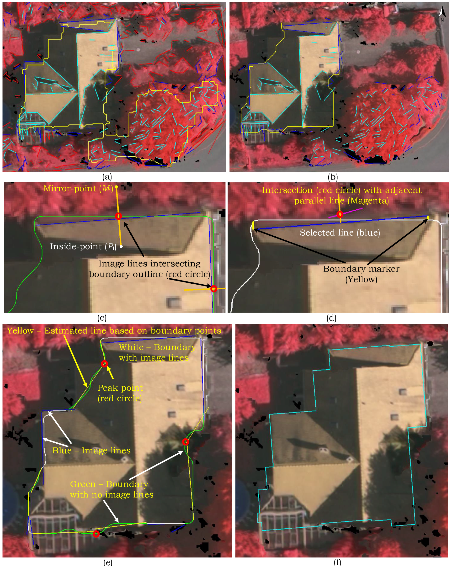
). We further incorporate LiDAR’s point density feature in different processes to make the proposed approach flexible and robust towards multiple data acquisition sources, e.g., airborne and mobile laser scanning systems. An adaptive local rather a global height threshold is utilised in one of the detection steps for fine delineation of the building boundaries. Moreover, a new boundary regularisation technique is also introduced which generates 2D building footprints using the spectral information (image lines) assuming buildings are rectilinear.
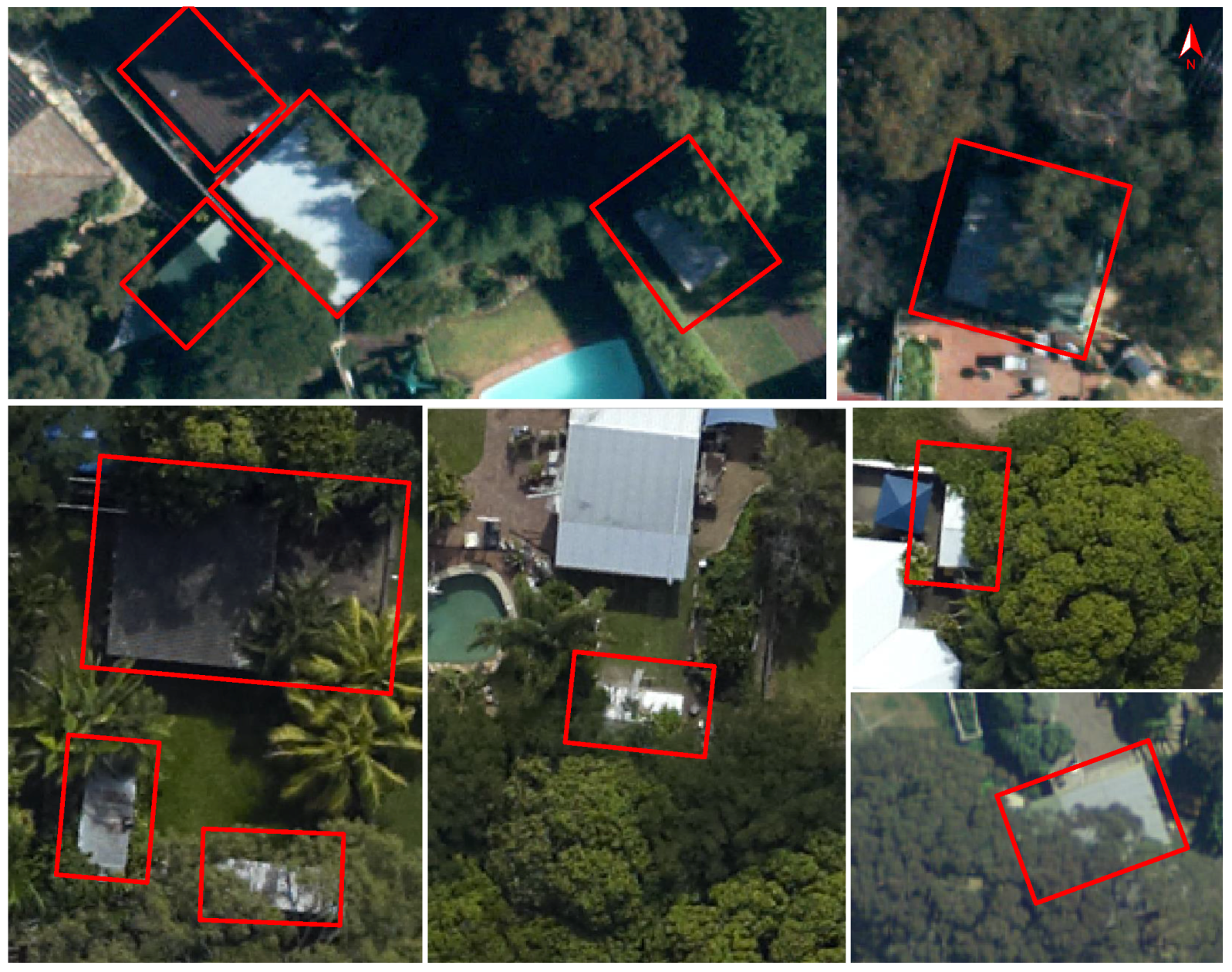
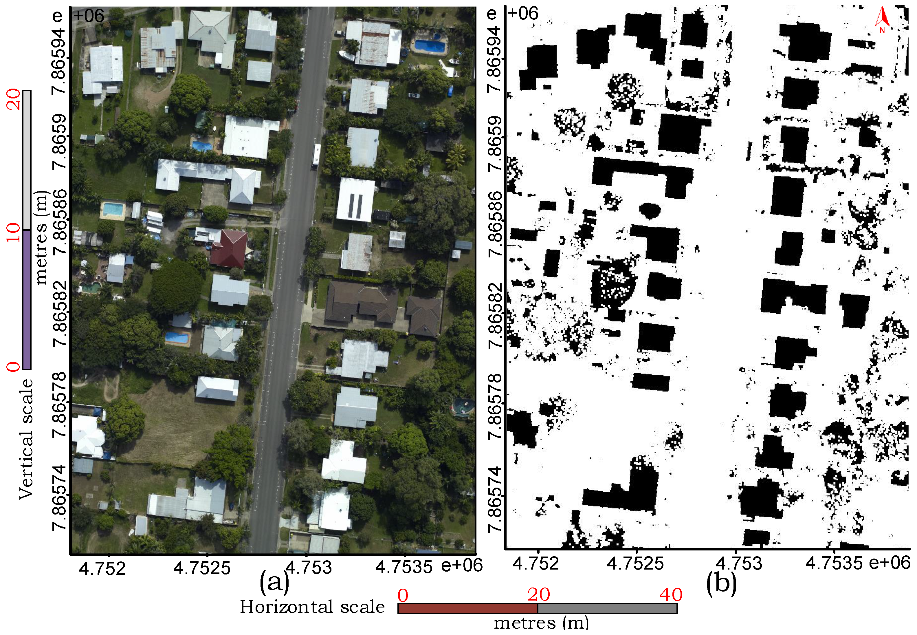
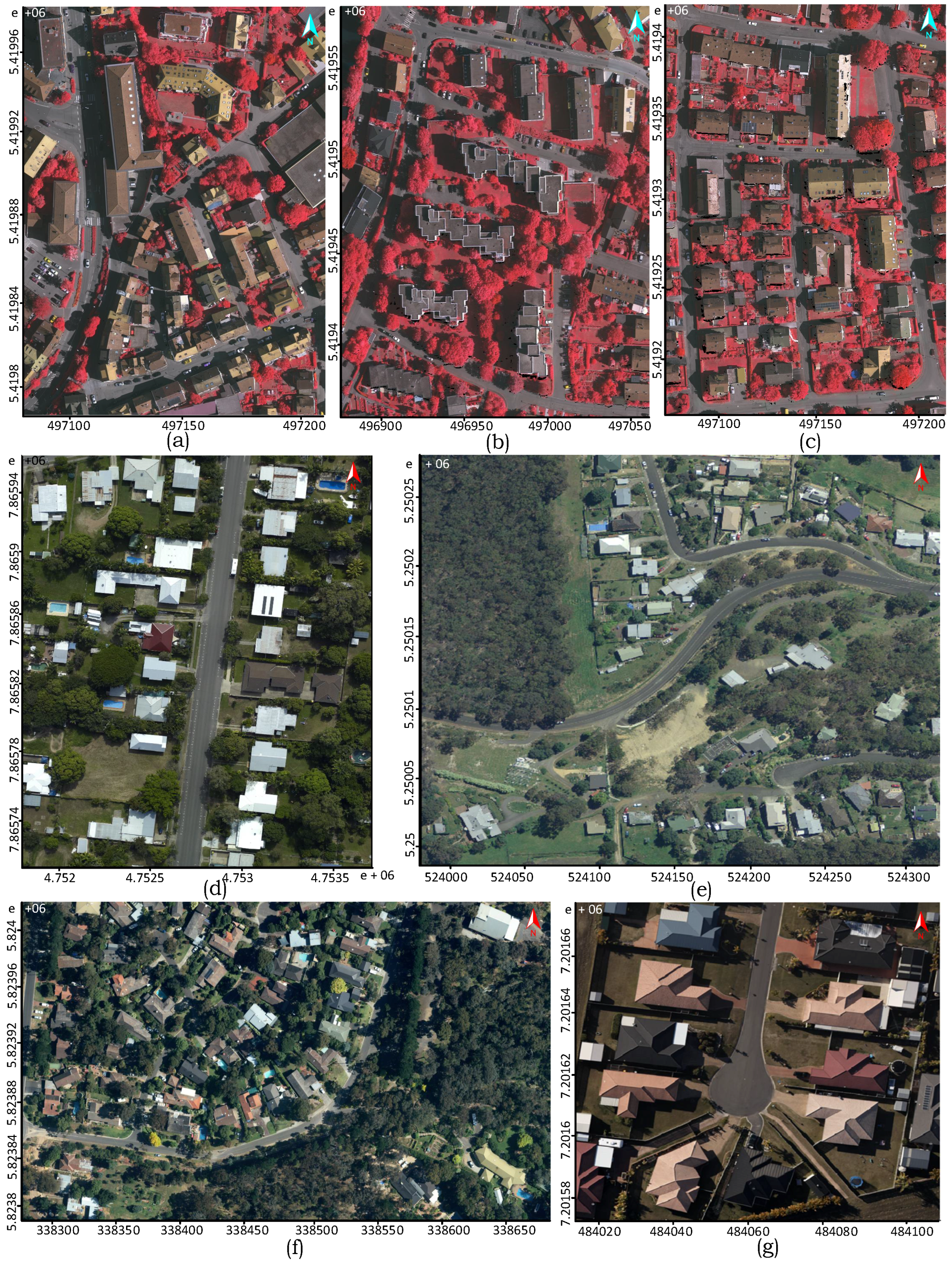
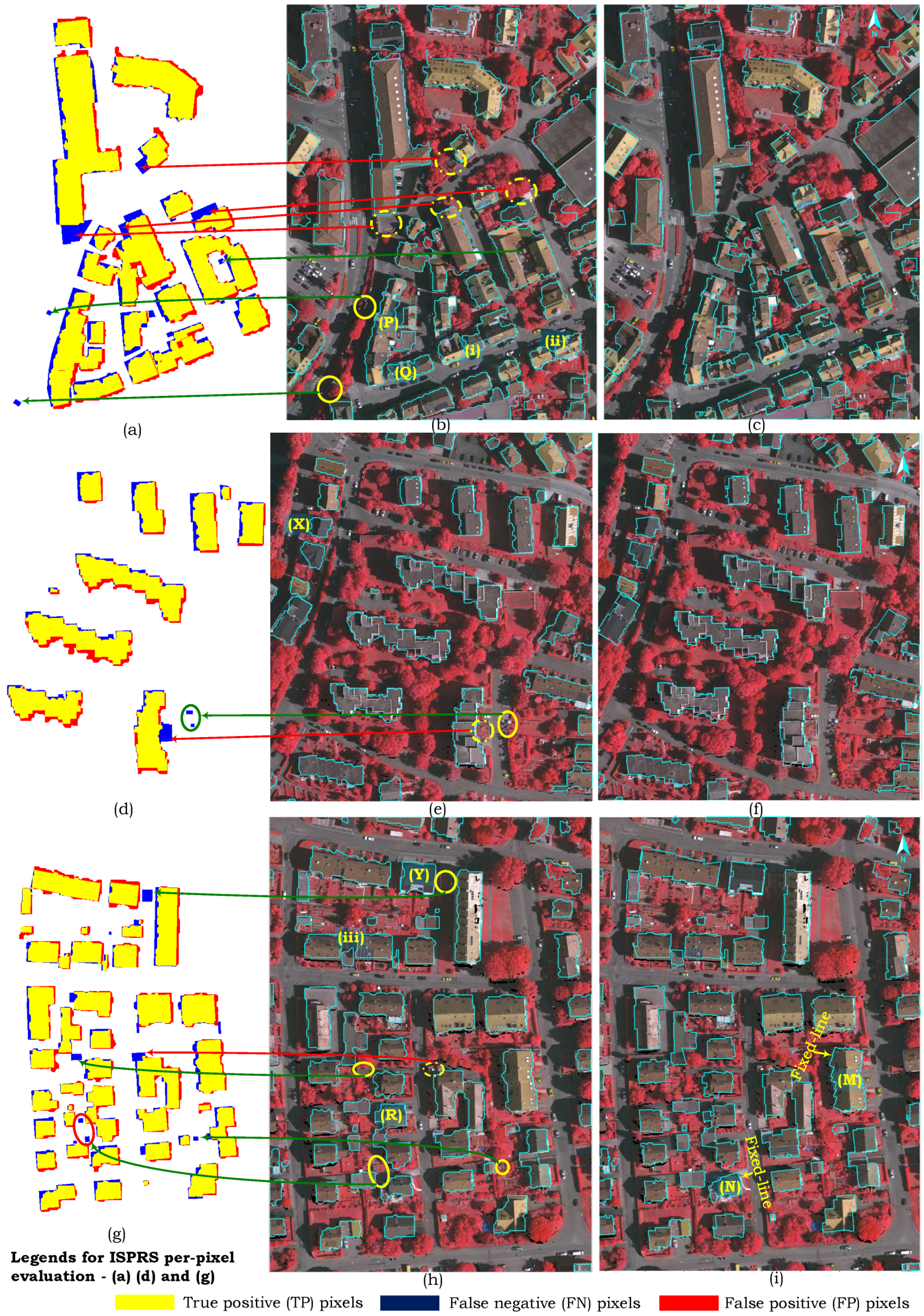
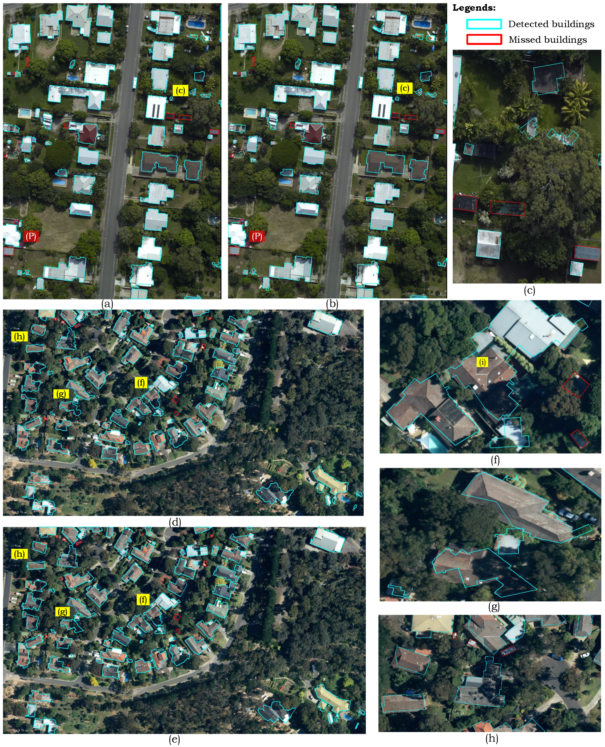
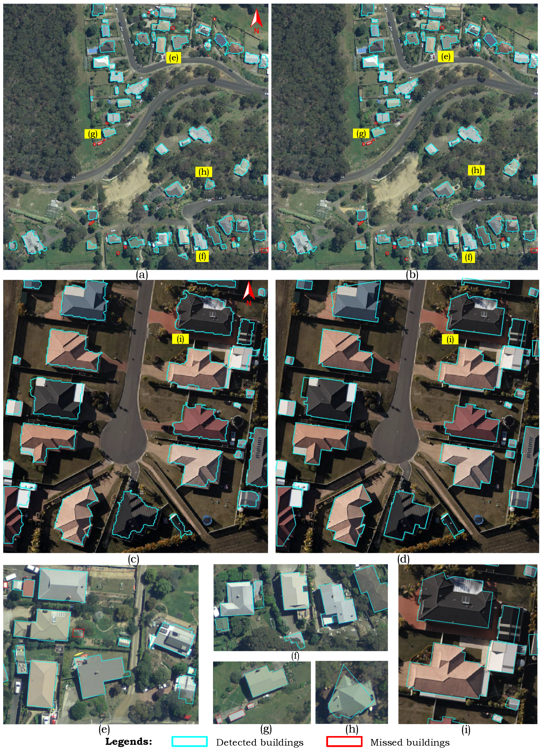
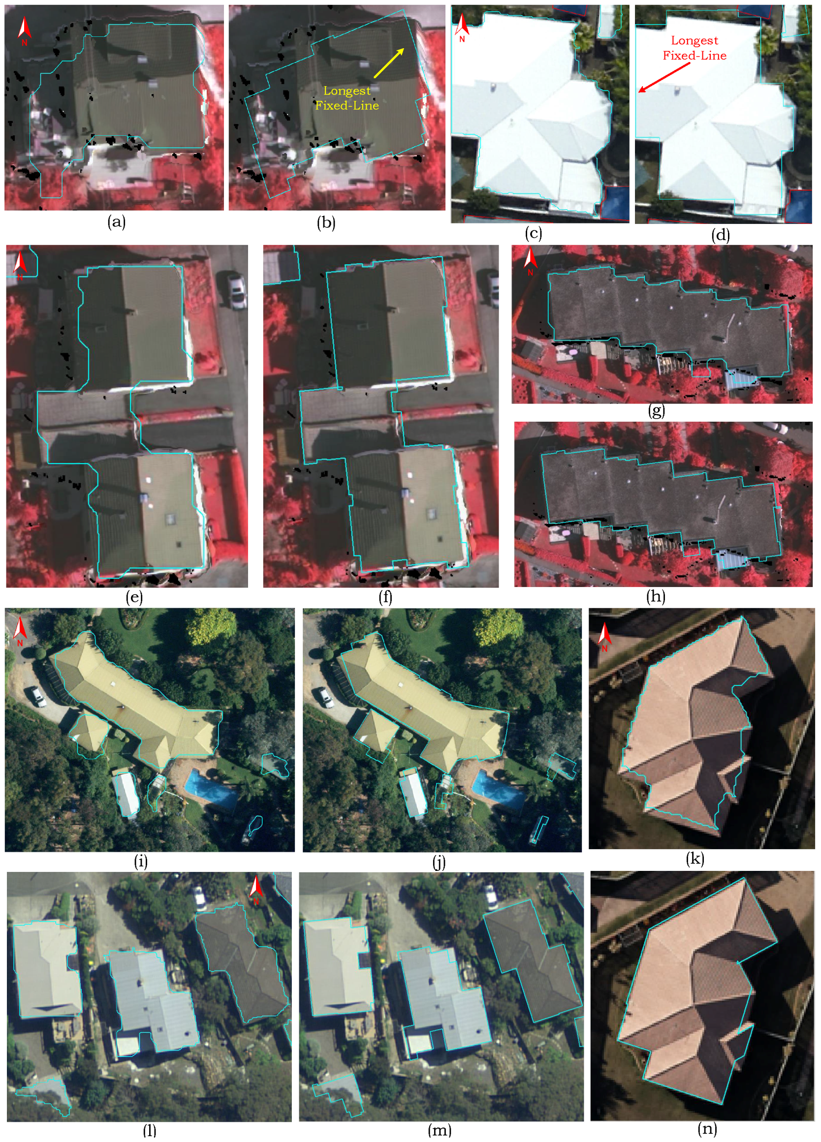
To meet the set objectives and evaluate rigorously, the proposed approach is tested using the ISPRS (German) and the Australian benchmark data sets. Compared to the ISPRS benchmark, the Australian data sets are found far complex and challenging due to hilly terrain (Eltham and Hobart), dense vegetation, shadows, occlusion, and low point density (1 point/m 2 ). Often, the buildings are covered with close by trees or shadows as described by real examples in Figure 1. The evaluation study, particularly on the Australian data sets, demonstrates the robustness of the proposed technique in regularising boundary and separating partly occluded buildings from connected vegetation and detecting small buildings apart from the larger ones.
The rest of the paper is organised as follows: Section 2 details the proposed building detection and the boundary regularisation techniques. Section 3 presents the performance study and discusses the experimental results using five test data sets followed by a comparative analysis. Finally, Section 4 concludes the paper.

2. Proposed Method

The workflow of the proposed approach consists of three stages as sketched in Figure 2. In the data preprocessing stage, several data metrics are generated to be used at later stages, which are namely the building mask and height difference data from the ALS, while entropy, NDVI, and image lines from the orthoimage. In the building detection stage, the candidate building regions are identified following a proposed graph-based line clustering process to remove the superfluous objects. Next, the buildings and their parts occluded or under shadows are identified and vegetation is eliminated using a proposed cell-based clustering process. Subsequently, the detected area is enlarged to reduce the misalignment between the aggregated data. Finally, the building footprints are generated using a new proposed building regularisation process.

2.1. Data Preprocessing

The proposed approach takes ALS data, orthoimagery, and a digital terrain model (DTM) as an input. For this study, DTM with 1 m horizontal resolution was available for each benchmark data set. Otherwise, it can be generated using any commercial software, such as MARS® explorer [33].

2.1.1. Test Data

Figure 3a presents a test data set, which is an Australian site named Aitkenvale (AV) in Queensland. The AV data set can be regarded as a moderately vegetated area containing complex building neighbourhood structures, small and occluded buildings, shadowed, impervious and transparent roofs, flat and gabled structures. It is, thereby, selected to evaluate the performance and illustrate the different processes of the proposed approach.
The test ALS data set has a point spacing of 0.17 m with 29.3 points/m 2 and the corresponding RGB colour orthoimage has a resolution of 0.05 m. The available orthoimages for the Australian sites were created using DTM. These data sets were registered using the mutual information based method [34], which exploits the statistical dependency between same- and multi-modal data sets to produce a similarity measure and uses LiDAR intensity in simultaneous registration. Nevertheless, the building roofs and tree tops are considerably displaced with respect to the LiDAR owing to the absence of true orthophotos.

2.1.2. ALS Generated Data

A building mask is generated using ALS data and ground height from DTM to divide the point cloud into the ground and non-ground points. For each point, a height threshold is calculated as h t = h g + h r f , where h g is the ground-height taken from DTM while h r f is a relief factor that separates the low height objects from the large height objects. For this study, h r f has been set to 1 m to keep low height objects [11], which classifies many points on bushes and low height trees as the non-ground points. Figure 3b shows the building mask where black region corresponds to elevated objects (buildings and trees) while white region represents bare-earth including roadside furniture, cars, and bushes.
Moreover, height difference data is generated by dividing the ALS data into a uniform grid of magnitude twice of the ALS data spacing. The method is explained with a sample image from test data set as shown in Figure 4a. If a cell contains only one laser point, the elevation of the point is assigned to the cell. Otherwise, the elevation of the laser point which is closest to the centre of the cell is assigned to the grid (see Figure 4b). In case, a cell has no laser point, the elevation of the grid is assigned zero height. Finally, the average height difference ΔH of each cell is computed by averaging the elevation differences of 8-connected neighbouring cells. ΔH will be used by the cell clustering process to delineate buildings and identify vegetation.

2.1.3. Aerial Image Generated Data

NDVI has been used extensively in literature to eliminate vegetation and classify scenes [15,22,25,35]. Nevertheless, many authors [2,15] emphasised to couple it with entropy, since NDVI alone is not a promising feature to handle shadows and coloured buildings. Therefore, texture information in the form of entropy [36] is utilised on the basis of the observation that trees are rich in texture and have higher surface roughness than building roofs [15]. Provided, a multispectral orthoimagery (RGBI) is not available, a pseudo-NDVI is then calculated from a colour orthoimage (RGB) following the process in [2,10,37], which assumes the three colour channels in the order of I-R-G to use the standard NDVI formula. From now onward, the term NDVI is referred to both NDVI and pseudo-NDVI.
Furthermore, using the method in [2], the image lines are extracted from the test input image and categorised into “edge” (building border), “ridge” (intersection of two roof planes), and “ground” classes sketched with “blue”, “cyan”, and “red” colours, respectively, in Figure 5. The structural lines define the shape and direction of a building. These can be used as a cue to differentiate vegetation and buildings and later, to generate building footprints in the building regularisation stage.

2.2. Building Detection

In this section, the building detection stage shown in Figure 2 is presented in more detail using the test data set.

2.2.1. Candidate Region Detection

Candidate building regions are identified using connected component analysis from the building mask and their boundaries are estimated using Moore-Neighborhood tracing algorithm [36], which provides an organised list of points (boundary) in the clockwise trace of connected pixels for an object in a binary image. Figure 6a shows the detected candidate regions, where each region is labelled and sketched in a different colour from its neighbour with the boundary black in colour. It is shown in Figure 6b that the extracted boundaries (from LiDAR-based building mask) are misaligned with the image (often over 1 m) due to misregistration between the aggregated data.
Similarly, Figure 6c shows the inaccuracy of the extracted objects where the large buildings are although detected but their boundaries are inaccurately delineated. It also shows the presence of several false objects on trees and an inaccurate inclusion of nearby vegetation into the building region. Moreover, due to the presence of dense vegetation between the buildings, they have been wrongly extracted as a single object (Label vi). Some complex situations are shown in Figure 6d with their corresponding locations marked with Labels (i)–(vi) in Figure 6c.

2.2.2. Line Clustering and False Candidate Elimination

To associate the lines (from image) and the candidate building regions (from the LiDAR-based building mask), a graph is constructed as part of this process. Each pixel of the building mask corresponds to a node. An edge exists between a pair of nodes if a pixel and its 3 × 3 neighbouring pixels are “black”, denoting a non-ground object. All these edges carry a weight equal to 1. However, if a pixel or the neighbouring pixels are “white” (ground-object), the corresponding nodes do not have any edge. Therefore, the resultant graph G is disconnected where each candidate region of the building mask corresponds to a strongly connected edge-weighted graph g, such that G = { g 1 , g 2 , , g n } with n describing the number of candidate regions.
Since the edge lines (blue) are substantially away from the borders of the non-ground objects due to data misalignment (see Figure 5b), therefore, a determinant point D p t is utilised along with G to cluster the image lines for each candidate region. D p t of a line can be either its midpoint P m i d , vertex, or inside-point P i n . This P i n is 1.5 m perpendicular offset point from line’s P m i d that is given by the line extraction process in [2] for each line. The line clustering process, with reference to Figure 7a, works as follows: A pool of candidate lines is created by defining a buffer region (cyan) using uniform matrix scaling transformation. Then, the longest line is chosen as a “seed”, such that its D p t resides within the region’s boundary. If no seed is found, the procedure continues to process the next building region. Finally, the candidate lines having finite distances from the seed are added into the cluster. Bellman-Ford algorithm, which computes the shortest path between two nodes, is used to calculate the distances between D p t ’s of the lines. The procedure continues until the pool is empty and process all the candidate regions iteratively. A candidate region which fails to cluster any line is removed for further investigation. Figure 7b shows the remaining candidate building regions with their clustered lines (it displays 307 candidate regions from an initial count of 936 from the building mask for brevity).

2.2.3. Cell Clustering for Building Detection and Vegetation Removal

It is a core process to distinguish urban objects, eliminate vegetation, and identify buildings partly occluded or under shadows besides the larger and the ones small in size. The features such as ΔH, N D V I and e n t r o p y are used to detect objects using a cell-based region growing process. To make the segmentation flexible and robust towards multiple data acquisition sources, e.g., airborne and mobile laser scanning systems [38], point cloud density per grid cell P d is combined with the preceding features. The test area is divided into a uniform grid structure and P d is computed in relation to the LiDAR’s resolution and the cell size, for example, P d for the AV data set is 7 (floor (29 × 0.25)) using a grid of size 0.25 m with 29 laser-points/m 2 , while of the German benchmark P d is 3 with a grid size of 1 m. The process is explained as follows with reference to Figure 8 (a sample occluded building Label (vi) in Figure 6):
The cells of a candidate building region are marked unused (blue circles in Figure 8a) and a seed cell is chosen i.e. an unused cell with the lowest ΔH. Its neighbours are found iteratively in a region growing fashion. Neighbouring cells are added to the cluster if their values for ΔH, P d , N D V I , and e n t r o p y are smaller than the user defined thresholds (see Table 1). After this, a cell with the smallest ΔH is chosen. This becomes the new seed cell. However, a seed that fails to grow is removed. Figure 8b shows the different clusters (filled in red) within the region’s boundary conceived during the cell clustering process.
An aerial data acquisition system sometimes fails to capture the laser returns from various parts of a single object. Therefore, a segmentation process using the ALS data alone potentially leads to an over-segmentation issue. To circumvent this limitation, the cell clustering process entirely uses N D V I and e n t r o p y if at maximum 25% of the total cells of a particular candidate region does not have any laser point. The seed cell is chosen with the lowest N D V I whereas a cell’s neighbours are chosen based on both N D V I and e n t r o p y rather than ALS features.
Finally, a rule-based procedure employing N D V I , e n t r o p y , and boundary intersection is used to identify a cluster within region’s boundary as a building or vegetation. It was found that the buildings under shadows or with coloured roofs have a higher N D V I value which could have been removed if a smaller threshold is employed. Therefore, N D V I t m a x is introduced which combines with image entropy to remove vegetation without eliminating any potential building. A cluster c is marked as a tree, if its boundary does not intersect with the boundary of the candidate region and N D V I c ¯ > N D V I t m a x OR N D V I c ¯ < N D V I t m a x AND e n t r o p y c ¯ > e n t r o p y t . Similarly, c is identified as a building, if its boundary intersects with the boundary of the candidate region and N D V I c ¯ < N D V I t OR N D V I c ¯ < N D V I t m a x AND e n t r o p y c ¯ < e n t r o p y t .
Figure 8c shows that two partially occluded buildings are identified and separated from the connected tree whereas the clusters within the region’s boundary are eliminated as “vegetation”. Similarly, few more detected buildings either occluded or under shadows, marked earlier in Figure 6, are shown in Figure 8d–h with their boundaries in cyan while the candidate regions’ boundaries in red. The final building positions are hence obtained by the cell clustering process after the vegetation elimination.

2.2.4. Building Area Enlargement

Owing to misalignment and a large height difference on the building perimeter, building edges are usually under-detected (Figure 9a and Figure 10a). That is compensated by claiming individual pixels based on NDVI, entropy and LiDAR height difference. An adaptive local height threshold is employed instead of a global threshold in area enlargement process by keeping into account the buildings with gabled, flat, and complex roofs. The process with reference to Figure 9 is described as follows:
A boundary pixel P b is first selected and its neighbouring pixels P n which are outside the current boundary (black) are determined. Subsequently, a concentric square of a grid-size (magenta) around P n is considered. If NDVI and entropy values of P n are less than their thresholds presented in Table 1, and the mean height within the square remains inside ±1 standard deviation of the building height (within the building boundary), it is then included as a new boundary pixel whereas P b is added into the building region. The building outline process continues until all the boundary pixels including the new ones are processed as described in Figure 9b,c. The building boundary before and after the enlargement process is presented in Figure 9d.
Figure 10a,b show building detection results before and after the pixel-based enlargement process. It is discernible that the final detected boundaries in Figure 10b cover rooftops well close towards the building edges and detects the building perimeter accurately. The same boundaries will be used eventually for the evaluation purpose. Since the building boundaries are independent, the clustering (line and cell-based) and area enlargement processes were executed in parallel to improve the performance.

2.3. Building Regularisation

Due to the point cloud sparsity, the extracted boundaries are jagged as shown in Figure 10b, which can be regularised by obtaining structural lines using MDL [5], but it is computationally intensive. However, the proposed regularisation approach employs image lines to regularise the boundary assuming buildings are rectilinear and adjacent edges should either be parallel or perpendicular. Since all possible image lines could not be extracted due to shadows and low contrast, this fact makes the German data set (Vaihingen) suitable to demonstrate the robustness of the regularisation technique. So, we choose a sample scene from Area 3, to explain the building footprint generation process.
The workflow of the regularisation process is shown in Figure 2. Figure 11a shows the boundary of the candidate building region (from the building mask) and classified image lines before application of the building detection steps described in Section 2.2. Figure 11b shows the clustered lines to the candidate building region and the refined building boundary after application of building detection procedure. The proposed building regularisation approach works in 3 steps: line selection, line estimation, and footprint generation.

2.3.1. Building Edge Selection

For each clustered line with its midpoint P m i d , we use its inside-point P i n and mirror-point P m i r to determine whether the line is a candidate line for the building boundary. For instance, with reference to Figure 11c, the image line (blue) exists near to the building perimeter, the perpendicular line from P m i r to P i n through P m i d intersects the extracted boundary (green), thus this line is a candidate boundary line. The corresponding boundary part of the selected line is also marked. Figure 11d shows the corresponding boundary parts within two yellow perpendicular lines through the end points of the selected line. This selected line can be from any class of “edge”, “ridge”, or “ground” due to the misalignment between the LiDAR-derived building boundary and image derived lines. All the candidate lines are determined iteratively. If a line fails to intersect building boundary, it is removed. If two or more candidate lines are found for a part of the boundary then the line that has the lowest mean perpendicular distance of the boundary points to the line, finally qualifies for the boundary part.

2.3.2. Edge Line Estimation

The edge lines are estimated only if the boundary points are left unmarked as illustrated by the green colour boundary in Figure 11e. These boundary points are first smoothed using the Gaussian function and then corner detection is carried out using the technique in [39]. We determine the curvature peaks (red circles in Figure 11e) that specify the locations where a considerable change in curve direction occurs. A straight line is then fitted to the boundary segments using a least-square technique such that the line is rotated by a half degree clockwise/anti-clockwise around its centre to minimise the mean perpendicular distance to boundary points. The estimated edge lines and the chosen image lines (yellow and blue respectively) can be seen in Figure 11e.

2.3.3. Building Footprint Generation

Assuming buildings mainly have two principal directions along its length and width, the lines at least 6 m long are considered as long lines [40]. The long lines from the image are kept fixed. If no image line exists, then the long estimated lines are kept fixed. In the case of only one single fixed line, all the other line segments are made parallel or perpendicular to it. The two closest small lines on both sides of a fixed line are adjusted first followed by the next two nearest small lines are tuned with reference to the last fixed lines. This process continues until all the lines are adjusted to a parallel and perpendicular relationship.
If there exist two or more fixed lines, the small lines in between are gradually made parallel or perpendicular to their nearest fixed lines. In the case where a small line is at an equal distance from the fixed lines, it is adjusted according to the fixed line with which it makes the smaller angle. Perpendicular lines are then introduced between the successive parallel lines. Finally, the regularised building boundary is generated by intersecting the consecutive lines. The regularised building footprint for the sample scene is sketched on the input image in Figure 11f.

3. Performance Evaluation

The performance of the proposed approach was tested on five data sets which have different LiDAR point densities, topography and surrounding conditions. The ISPRS benchmark data set, Vaihingen, Germany has three areas whereas the other four data sets have one area each captured over different geographic locations in Australia.

3.1. Evaluation Methods

Due to a current lack of a uniform evaluation system [41], the objective evaluation followed both the threshold-based system [41] adopted by the ISPRS and an automatic and threshold-free evaluation system [42] for the German and the Australian data sets, respectively. Both the evaluation systems perform three categories of evaluations: object-based, pixel-based, and geometric, where each category uses several metrics. For example, the object-based metrics (completeness, correctness, quality, under- and over-segmentation errors, and reference cross-lap rates) evaluate the performance by counting the number of buildings, while the pixel-based metrics (completeness, correctness, quality, area-omission, and area-commission errors) measure the detection accuracy by counting the number of pixels. In addition, the geometric metric (root mean square error i.e., RMSE) indicates the accuracy of the extracted boundaries with respect to the reference entities. For all the data sets, the minimum areas for large and small buildings have been set to 50 m 2 and 10 m 2 , respectively.

3.2. Benchmark Data Sets

The first data set is Vaihingen (VH), from the ISPRS benchmark that has three test sites as presented in Figure 12a–c. Each area has a point density of 3.5, 3.9 and 3.5 points/m 2 , respectively. Area 1 is situated in the centre of the city and characterised by dense construction consisting of historic buildings having complex shapes. Area 2 is characterised by a few high-rise residential buildings surrounded by trees. Finally, Area 3 is purely residential, with detached houses and many surrounding trees. The number of buildings (larger than 2.5 m 2 ) in these three areas are 37, 14, and 56, respectively.
The four Australian data sets, Aitkenvale (AV), Eltham (EL), Hobart (HT), and Hervey Bay (HB), have point densities of 29.3, 4.8, 1.6, and 12 points/m 2 , respectively. Topographically, the AV and HB areas are flat while EL and HT are hilly containing mostly residential buildings with different level of vegetation. The AV, EL and HT data sets have dense vegetation, where many of the buildings are severely occluded by the surrounding trees. These test areas, shown in Figure 12d–g, cover 214 × 159 m 2 , 393 × 224 m 2 , 303 × 302 m 2 , and 108 × 104 m 2 , respectively. The AV contains 63 buildings (four are between 4 to 5 m 2 and 10 are between 5 to 10 m 2 ). The EL data set contains 75 buildings (nine are less than 10 m 2 , including five within 3 to 5 m 2 ). The HT data set has 69 buildings (thirteen are less than 10 m 2 , including four within 1 to 5 m 2 ). The HB data set contains 28 buildings (three are between 4 to 5 m 2 and six are between 5 to 10 m 2 ). The reference data sets include parking shades, huts, and shelter umbrellas as buildings during evaluation provided the height is more than the threshold (1 m).

3.3. Results and Discussion

Section 3.3.1 and Section 3.3.2 describe and discuss the evaluation results of our proposed technique on the ISPRS benchmark and the Australian data sets.

3.3.1. ISPRS Benchmark Results

Table 2 and Table 3 show the official per-object and per-area level evaluation results for the three test areas of the benchmark data set. Figure 13 shows the per-pixel level visual evaluation of all the test areas (column 1) for the building delineation technique (column 2) and their corresponding regularisation outcome (column 3). The detailed quality measures for building delineation technique before and after the regularisation can be found on the ISPRS portal [43] under detection with acronym Fed_1 and Fed_2, respectively.
Considering all the buildings, Table 2 shows that the overall object-based completeness and correctness before regularisation are 83.87% and 95.80%, respectively. However, the buildings eliminated during the mask generation process, showed with “green” arrows in Figure 13a,d,g became a bottleneck in a relatively reduced performance. Howbeit, 100% object-based accuracy was achieved on the large buildings. Since the overlap areas of the resultant and reference polygons after the regularisation process were not greatly changed, therefore, a substantial increase in per-object evaluation accuracy was not achieved. Table 3 shows the per-area evaluation (completeness and correctness ≃ 88% and 85%, respectively) of the proposed detection before regularisation in Area 2 and Area 3. However, per-area completeness in Area 1 was lower (84.9%) because few carports below the height threshold, marked with yellow dashed circles in Figure 13b and one in Area 3 (Figure 13h), were eliminated by the building mask generation process.
During the cell clustering process, the cells lying partially on the building perimeter were included into the region. That is why, few very close buildings were combined unexpectedly (marked as P, Q and R) apart from the false positive pixels as shown in Figure 13. This could have been avoided by analysing the white pixels from the building mask during the region growing. Nevertheless, the proposed approach extracted several close buildings at a higher accuracy as shown in Figure 13b,h with Labels (i)–(iii). Moreover, two buildings Label X and Y as shown in Figure 13e,h, respectively were extracted completely using the proposed cell clustering process although major parts of the buildings do not have any LiDAR data recorded. Results in Table 2 further indicate that the proposed approach is absolutely free from over- (1:M) and many-to-many (M:N) segmentation errors, albeit there are few under-segmentation cases.
Table 3 shows that the regularisation process improved the per-area completeness, correctness, and quality on top of building detection results. This increase might be substantial if the image lines could come in place of boundary segments, which are more accurate representative of the building perimeter than the ALS boundary. However, a slight decrease in VH3 correctness after the regularisation was observed because the lines and their intersections (corners) were shifting from their actual positions during the regularisation. Notably, the regularisation process obtained a higher planimetric accuracy that reached up to two times the horizontal point spacing of the ALS data. Overall, it can be established from the evaluation performance that the proposed delineation together with regularisation process not only can eliminate vegetation, extract building as well as their parts from the connected trees but also regularise the boundary with 98.57% average objective correctness.

3.3.2. Australian Results

Table 4 and Table 5 present object- and pixel-based evaluation of the detection technique before and after the regularisation using the threshold-free evaluation system. Figure 14 and Figure 15 show the extracted buildings and their corresponding building footprints for the AV, EL, HT, and HB data sets. The proposed detection extracted 55, 68, 62, and 22 buildings out of 65, 75, 69, and 22 reference buildings in the AV, EL, HT, and HB data sets, respectively.
Table 4 shows that the object-based completeness of HT on all the buildings was comparatively lower than that of AV and EL. The reason was the missing buildings (marked “red”) caused by severe occlusion (Figure 14c,f and Figure 15e) and transparent roof material (Figure 15g). The results further show that the buildings over 50 m 2 were extracted with 100% objective completeness and correctness while nearly equal average completeness (≃ 95%) was achieved on the buildings over 10 m 2 .
Figure 14c,f–h show scenarios where non-occluded building parts were extracted after eliminating the connected vegetation. However, two very close buildings in EL, Label (i) in Figure 14f, were unexpectedly merged due to a small connecting region. Such complex cases increased cross-lap rate (under-segmentation) in EL than AV and HT as given in Table 4. This could be prevented by taking care of white pixels between the connected regions from the building mask. Since the overlap areas of the resultant and reference polygons in before and after the regularisation process was not changed much, therefore, objective evaluation was nearly the same as shown in Table 4.
Table 5 shows the pixel-based evaluation (completeness and correctness ≃87% and 95%) before regularisation for AV, HT, and HB. However, a relatively lower completeness in EL (80.57%) than others caused by missing fewer buildings which were under severe occlusion and was evident from the high area omission errors. For the buildings larger than 50 m 2 , an average completeness and correctness of about 87% and 95% were achieved, while the similar were obtained for buildings over 10 m 2 . More than 2% rise in average completeness was recorded after the regularisation process when all the buildings were considered. Yet, the planimetric accuracy was compromised, since the regularised lines and their intersections were repositioning to generate a regularised boundary. Nevertheless, an average pixel-based completeness increased significantly in HB from 86.95% to 91.80% after the regularisation on all the buildings as shown in Table 5. The obvious reason was that major parts of the delineated boundary had a respective image line which gave rise to accuracy.
The performance of the proposed approach is demonstrated using several data sets which have transparent to complex structure buildings with varying sizes, flat to hilly terrain, low to dense vegetation, and different ALS resolutions (1 to 29 points/m 2 ). Qualitative (figures) and quantitative (Table 2, Table 3, Table 4 and Table 5) results show that the proposed detection approach can eliminate vegetation and extract buildings as well as their non-occluded parts from the complex scenes at a high object- and pixel-based accuracy. A constantly higher (>95%) correctness suggests that the proposed detection technique is robust. Moreover, the applicability of the regularisation process after the detection is effective in the useful generation of the building footprints.

3.4. Comparative Analysis

The proposed method is automatic and data-driven that integrates LiDAR and orthoimagery. It predominantly uses LiDAR to create the building mask and building extraction. From the ISPRS portal and the classified methods in [44], we select those which (1) use both LiDAR and image; (2) in which pixel- and point-based processing is equally important; (3) automatic; and (4) unsupervised and data-driven [44]. Due to a lack of integrated methods complying the above criteria, 2 supervised integrated (Criteria 1–3) and 2 LiDAR only (Criteria 2–4) methods are also chosen as shown in Table 6. The quantitative evaluation of the German data set (Area 1, Area 2, and Area 3) for KNTU_mod, Whuz, IIST, Mon2, and the proposed detection and regularisation approach (FED_2) are available on the ISPRS’ website, however, Yang’s [45] results are taken from the paper. To the best of our knowledge, the only method evaluated using the evaluation system in [42] on the Australian data sets is MA [11] and hence, chosen for the comparative study to conduct a fair evaluation.
The comparison between FED_2 and other methods is presented in Table 7 and Table 8, where bold numbers show better or equal performance of our technique. FED_2 performed significantly better on the Australian data sets which are characterised more complex than the ISPRS benchmark due to dense vegetation, shadows, and topography. Likewise, FED_2 achieved similar or better object and area level completeness and correctness than the counterparts in all the German areas. Although, in Area 1, Mon2 offered better object completeness, since it captured the carports at ground-height due to more accurate DTM, however, high per-object correctness was obtained by FED_2 (see Table 7), which is an indicator of a method’s robustness. Moreover, the proposed method had better objective completeness than Yang which had more per-area completeness on Area 1. Besides FED_2 performed better in Area 2 than fellow methods, Mon2 achieved slightly better per-object completeness in Area 3. Nevertheless, FED_2 achieved higher per-area and better per-object completeness on large buildings in Area 3.
Table 7 further shows that large buildings (50 m 2 ) were extracted with 100% completeness than Yang and Mon2, who missed large buildings from Area 3 while IIST from Areas 1 and 3. The same also shows that IIST performed poorly on all the Areas in German data set due to an inappropriate integration of features extracted from LiDAR and image. Notably, FED_2 was mainly free from over- and many-to-many segmentation errors, but had few under-segmentation cases, unlike Yang which suffered from many-to-many and under-segmentation. When compared with supervised methods which are trained to perform a better classification, the proposed approach achieved better per-object completeness and correctness in all the areas except Area 3. Likewise, it demonstrated better in per-area level except in Area 1 where KNTU_mod had better completeness and correctness. However, Whuz performed consistently poor on all the Areas in German data set and even missed buildings larger than 50 m 2 from Areas 1 and 3. Since the segmentation results of IIST, KNTU_mod, and Whuz were not available, therefore, a comparative discussion was not provided.
FED_2 achieved better object and area level accuracy than MA on the Australian data sets as shown in Table 8. However, in EL, per-area completeness of MA was marginally better but performed poorly (per-object) in AV due to missing small buildings. Nevertheless, FED_2 offered high completeness and correctness on all the data sets but underwent through a lower planimetric accuracy than MA. It was concluded that FED_2 was found quite robust under complex scenarios on the Australian data sets and achieved higher completeness and correctness. However, it achieved better or equal performance except few cases on the ISPRS benchmark data sets with a constantly high correctness.

3.5. Implications of the Regularisation Technique

Although, per-area completeness increased after the regularisation process, but could not achieve the expectation level (above 95%). On the contrary, the planimetric accuracies of the 2D footprints for the AV, HT, and HB data sets were adversely affected as shown in Table 5. The phenomenon is explained through samples from VH Area 3 and AV data sets in Figure 16a,c, respectively. The positions of these buildings were labelled (N) and (P) in former Figure 13h,i and Figure 14a,b, respectively.
As described under Section 2.3.3, the regularisation process begins with the selection of a longest fixed line (see Figure 16b,d) and adjusts the nearby lines with respect to it. A wrong selection of the fixed line may deviate the generated footprint from the building’s orientation or if the coincident lines are fixed and do not comply any parallel or perpendicular relation, such segments are joined without any adjustment. Thereby, it increases the RMSE. This issue can be resolved by minimising the line to the boundary distance during fixed line selection and line adjustment. Besides, some additional corners are observed in a regularised boundary as a result of the vertical lines introduced to construct a building footprint. This issue can be avoided by finding the intersection points of nearby lines (image and estimated) and adjusting them into a parallel or perpendicular relationship instead of inserting new lines. For observation, building footprints of few sample detected buildings from VH Area 3, VH Area 2, EL, HT, and HB data sets are sketched in Figure 16e–n. It shows that the applicability of the regularisation process even for complex building structures after the detection is effective in the useful generation of building footprints.

3.6. Limitations of the Proposed Detection

The objects either made of transparent materials which allow the laser to penetrate through to the ground or lower than the height threshold (1 m) are eliminated by the mask generation process. Therefore, such objects will not be extracted. The construction of transparent roofs is not widely practised and even if exist, are mainly used for sheds and huts and not for main buildings, so does not significantly impact the application of the proposed building detection technique. Moreover, irregular buildings, such as domes, although may be detected in the building mask, they will be either wrongly regularised as rectilinear buildings when long lines are found from the orthoimage or eliminated due to the absence of long image lines. Also, small buildings with area less than the grid’s cell-size (1 m 2 ) will be eliminated by the clustering processes.

4. Conclusions and Outlook

A building detection and footprint generation technique is presented here, which is fully data-driven and automatic. The candidate building regions are first identified using connected component analysis. Then, the buildings are extracted including partly occluded and shadowed after the vegetation removal through the grid index structure and multisource data. Finally, the building footprints are generated using the image lines and the extracted building boundaries.
The performance of the proposed technique is tested on several data sets having different point densities (1 to 29 points/m 2 ), topographic and vegetation conditions. Results showed that it not only can extract small, partially occluded and shadowed buildings but can generate footprints irrespective of the surrounding complexity. The proposed method offers high detection rates even in the presence of moderate registration error between the ALS data and the orthoimagery. Furthering to the performance, the experimental results demonstrated that our method is completely free from many-to-many and over-segmentation errors, which is imperative to obtain high objective accuracy. When compared with six existing methods, the proposed technique performed better than the counterparts with the correctness of above 95%. Additionally, the building outlines produced here are regularised in contrast to recent methods which generate only ragged boundaries.
Due to the mask generation process, the buildings below the height threshold and transparent materials were removed and hence, were not detected. In addition, the planimetric accuracy of the regularised boundary was affected because of the registration error between LiDAR and image. Hence, it would be interesting to cluster the image lines using the delineated boundary before the regularisation process begins. The per-area and planimetric accuracy of the building footprints are likely to improve. Moreover, the research to extract the transparent buildings by using LiDAR intensity and image gradient is under investigation. The proposed method applied both the radiometric and geometric clues in order to detect buildings in complex situations, especially when buildings were connected with neighbouring dense vegetation and partially occluded. Another important geometric clue that can also be applied is the general planarity principle, which states that a building roof consists of one or more large planar segments while a tree does not [11]. Our future investigation on 3D building modelling and regularisation will use this clue as well. This is also planned to test the applicability of the proposed approach on more data sets having large registration errors.

Acknowledgments

The research is supported under the Discovery Early Career Researcher Award by the Australian Research Council (project number DE120101778). The Aitkenvale and Hervey Bay data sets were provided by Ergon Energy (http://www.ergon.com.au) in Queensland, Australia. The Hobart and Eltham data sets were provided by Photomapping Services and Department of Environment and Primary Industries of Victoria, Australia, respectively. The Vaihingen data set was provided by the German Society for Photogrammetry, Remote Sensing and Geoinformation (DGPF) [49]. Special thanks go to Markus Gerke of the International Training Centre (ITC), Netherlands, for evaluating the building outlines extracted with the proposed technique before and after regularisation stage.

Author Contributions

Syed Ali Naqi Gilani has developed, implemented and conducted the tests on the benchmark and the Australian data sets. In addition, he has written the paper. M. Awrangjeb has supervised the research and reviewed the paper for the organisation, clarification and English corrections. G. Lu proofread the paper and suggested improvements in writing style and its structure.

Conflicts of Interest

The authors declare no conflict of interest.

References

  1. Al-Khudhairy, D.H. Geo-spatial information and technologies in support of EU crisis management. Int. J. Digit. Earth 2010, 3, 16–30. [Google Scholar] [CrossRef]
  2. Awrangjeb, M.; Zhang, C.; Fraser, C.S. Automatic extraction of building roofs using LiDAR data and multispectral imagery. ISPRS J. Photogramm. Remote Sens. 2013, 83, 1–18. [Google Scholar] [CrossRef]
  3. Sahar, L.; Krupnik, A. Semiautomatic extraction of building outlines from large-scale aerial images. Photogramm. Eng. Remote Sens. 1999, 65, 459–466. [Google Scholar]
  4. Lin, C.; Huertas, A.; Nevatia, R. Detection of buildings using perceptual grouping and shadows. IEEE Comput. Soc. Conf. Comput. Vis. Pattern Recognit. 1994, 62–69. [Google Scholar]
  5. Weidner, U.; Förstner, W. Towards automatic building extraction from high-resolution digital elevation models. ISPRS J. Photogramm. Remote Sens. 1995, 50, 38–49. [Google Scholar] [CrossRef]
  6. Xiao, J.; Gerke, M.; Vosselman, G. Building extraction from oblique airborne imagery based on robust façade detection. ISPRS J. Photogramm. Remote Sens. 2012, 68, 56–68. [Google Scholar] [CrossRef]
  7. Fradkin, M.; Maìtre, H.; Roux, M. Building detection from multiple aerial images in dense urban areas. Comput. Vis. Image Underst. 2001, 82, 181–207. [Google Scholar] [CrossRef]
  8. Khoshelham, K.; Nardinocchi, C.; Frontoni, E.; Mancini, A.; Zingaretti, P. Performance evaluation of automated approaches to building detection in multi-source aerial data. ISPRS J. Photogramm. Remote Sens. 2010, 65, 123–133. [Google Scholar] [CrossRef]
  9. Li, Y.; Wu, H. An improved building boundary extraction algorithm based on fusion of optical imagery and LIDAR Data. Optik 2013, 124, 5357–5362. [Google Scholar] [CrossRef]
  10. Rottensteiner, F.; Trinder, J.; Clode, S.; Kubik, K. Using the Dempster-Shafer method for the fusion of LiDAR data and multi-spectral images for building detection. Inf. Fusion 2005, 6, 283–300. [Google Scholar] [CrossRef]
  11. Awrangjeb, M.; Fraser, C.S. Automatic segmentation of raw LiDAR data for extraction of building roofs. Remote Sens. 2014, 6, 3716–3751. [Google Scholar] [CrossRef]
  12. Zhang, Q.; Qin, R.; Huang, X.; Fang, Y.; Liu, L. Classification of ultra-high resolution orthophotos combined with DSM using a dual morphological top hat profile. Remote Sens. 2015, 7, 16422–16440. [Google Scholar] [CrossRef]
  13. Zhou, G.; Song, C.; Simmers, J.; Cheng, P. Urban 3D GIS from LiDAR and digital aerial images. Comput. Geosci. 2004, 30, 345–353. [Google Scholar] [CrossRef]
  14. Qin, R.; Fang, W. A hierarchical building detection method for very high resolution remotely sensed images combined with DSM using graph cut optimization. Photogramm. Eng. Remote Sens. 2014, 80, 873–883. [Google Scholar] [CrossRef]
  15. Chen, L.; Zhao, S.; Han, W.; Li, Y. Building detection in an urban area using lidar data and QuickBird imagery. Int. J. Remote Sens. 2012, 33, 5135–5148. [Google Scholar] [CrossRef]
  16. Yong, L.; Huayi, W. Adaptive building edge detection by combining LiDAR data and aerial images. Int. Arch. Photogramm. Remote Sens. Spat. Inf. Sci. 2008, XXXVII, 197–202. [Google Scholar]
  17. Sampath, A.; Shan, J. Building boundary tracing and regularization from airborne LiDAR point clouds. Photogramm. Eng. Remote Sens. 2007, 73, 805–812. [Google Scholar] [CrossRef]
  18. Habib, A.; Kwak, E.; Al-Durgham, M. Model-based automatic 3d building model generation by integrating lidar and aerial images. Arch. Photogramm. Cartogr. Remote Sens. 2011, 22, 187–200. [Google Scholar]
  19. Zhou, G.; Zhou, X. Seamless fusion of LiDAR and aerial imagery for building extraction. IEEE Trans. Geosci. Remote Sens. 2014, 52, 7393–7407. [Google Scholar] [CrossRef]
  20. Haala, N.; Walter, V. Automatic classification of urban environments for database revision using lidar and color aerial imagery. Int. Arch. Photogramm. Remote Sens. 1999, XXXII, 76–82. [Google Scholar]
  21. Demir, N.; Poli, D.; Baltsavias, E. Extraction of buildings using images & LIDAR data and a combination of various methods. Int. Arch. Photogramm. Remote Sens. Spat. Inf. Sci. 2009, XXXVIII, 71–76. [Google Scholar]
  22. Rottensteiner, F.; Trinder, J.; Clode, S.; Kubik, K. Building detection using LiDAR data and multispectral images. DICTA 2003, 2, 673–682. [Google Scholar]
  23. Vu, T.; Yamazaki, F.; Matsuoka., M. Multi-scale solution for building extraction from LIDAR and image data. Int. J. Appl. Earth Obs. Geoinf. 2009, 11, 281–289. [Google Scholar] [CrossRef]
  24. Khoshelham, K.; Nedkov, S.; Nardinocchi, C. A comparison of bayesian and evidence-based fusion methods for automated building detection in aerial data. Int. Arch. Photogramm. Remote Sens. Spat. Inf. Sci. 2008, XXXVII, 1183–1188. [Google Scholar]
  25. Grigillo, D.; Kanjir, U. Urban object extraction from digital surface model and digital aerial images. ISPRS Ann. Photogramm. Remote Sens. Spat. Inf. Sci. 2012, I, 215–220. [Google Scholar] [CrossRef]
  26. Alharthy, A.; Bethel, J. Heuristic filtering and 3D feature extraction from LIDAR data. Int. Arch. Photogramm. Remote Sens. Spat. Inf. Sci. 2002, XXXIV, 29–34. [Google Scholar]
  27. Fu, C.S.; Shan, J. 3-D building reconstruction from unstructured distinct points. Int. Arch. Photogramm. Remote Sens. 2004, XXXV, 553–558. [Google Scholar]
  28. Ma, R. DEM generation and building detection from LiDAR data. Photogramm. Eng. Remote Sens. 2005, 71, 847–854. [Google Scholar] [CrossRef]
  29. Lach, S.R.; Kerekes, J.P. Robust extraction of exterior building boundaries from topographic LiDAR data. IEEE Int. Geosci. Remote Sens. Symp. 2008, 2, 85–88. [Google Scholar]
  30. Sohn, G.; Huang, X.; Tao, V. Using a binary space partitioning tree for reconstructing polyhedral building models from airborne LiDAR data. Photogramm. Eng. Remote Sens. 2008, 74, 1425–1438. [Google Scholar] [CrossRef]
  31. Wei, S. Building boundary extraction based on lidar point clouds data. Int. Arch. Photogramm. Remote Sens. Spat. Inf. Sci. 2008, XXXVII, 157–161. [Google Scholar]
  32. Gilani, S.; Awrangjeb, M.; Lu, G. Fusion of LiDAR data and multispectral imagery for effective building detection based on graph and connected component analysis. Int. Arch. Photogramm. Remote Sens. Spat. Inf. Sci. 2015, I, 65–72. [Google Scholar] [CrossRef]
  33. MERRICK® & Company. The Merrick Advanced Remote Sensing (MARS®). Available online: http://www.merrick.com/Geospatial/Software-Products/MARS-Software (accessed on 29 December 2015).
  34. Parmehr, E.G.; Fraser, C.S.; Zhang, C.; Leach, J. Automatic registration of optical imagery with 3D LiDAR data using statistical similarity. ISPRS J. Photogramm. Remote Sens. 2014, 88, 28–40. [Google Scholar] [CrossRef]
  35. Gerke, M.; Xiao, J. Fusion of airborne laserscanning point clouds and images for supervised and unsupervised scene classification. ISPRS J. Photogramm. Remote Sens. 2014, 87, 78–92. [Google Scholar] [CrossRef]
  36. Gonzalez, R.C.; Woods, R.E.; Eddins, S.L. Digital Image Processing Using MATLAB, 2nd ed.; Prentice Hall: Upper Saddle River, NJ, USA, 2003. [Google Scholar]
  37. Awrangjeb, M.; Ravanbakhsh, M.; Fraser, C. Automatic building detection using LiDAR data and multispectral imagery. In Proceedings of the 2010 International Conference on Digital Image Computing: Techniques and Applications (DICTA), Sydney, NSW, Australia, 1–3 December 2010; pp. 45–51.
  38. Lari, Z.; Habib, A. An adaptive approach for the segmentation and extraction of planar and linear/cylindrical features from laser scanning data. ISPRS J. Photogramm. Remote Sens. 2014, 93, 192–212. [Google Scholar] [CrossRef]
  39. Awrangjeb, M.; Lu, G.; Fraser, C.S.; Ravanbakhsh, M. A fast corner detector based on the chord-to-point distance accumulation technique. In Proceedings of the Digital Image Computing: Techniques and Applications, 2009. DICTA ’09, Melbourne, VIC, Australia, 1–3 December 2009; pp. 519–525.
  40. Awrangjeb, M.; Lu, G.; Fraser, C. Automatic building extraction from LiDAR data covering complex urban scenes. Int. Arch. Photogramm. Remote Sens. Spat. Inf. Sci. 2014, I, 25–32. [Google Scholar] [CrossRef]
  41. Rutzinger, M.; Rottensteiner, F.; Pfeifer, N. A comparison of evaluation techniques for building extraction from airborne laser scanning. IEEE J. Sel. Top. Appl. Earth Observ. Remote Sens. 2009, 2, 11–20. [Google Scholar] [CrossRef]
  42. Awrangjeb, M.; Fraser, C. An automatic and threshold-free performance evaluation system for building extraction techniques from airborne LiDAR data. IEEE J. Sel. Top. Appl. Earth Obs. Remote Sens. 2014, 7, 4184–4198. [Google Scholar] [CrossRef]
  43. ISPRS. Results: ISPRS Test Project on Urban Classification and 3D Building Reconstruction. Available online: http://www2.isprs.org/commissions/comm3/wg4/results.html (accessed on 29 December 2015).
  44. Rottensteiner, F.; Sohn, G.; Gerke, M.; Wegner, J.D.; Breitkopf, U.; Jung, J. Results of the ISPRS benchmark on urban object detection and 3D building reconstruction. ISPRS J. Photogramm. Remote Sens. 2014, 93, 256–271. [Google Scholar] [CrossRef]
  45. Yang, B.; Xu, W.; Dong, Z. Automated extraction of building outlines from airborne laser scanning point clouds. IEEE Geosci. Remote Sens. Lett. 2013, 10, 1399–1403. [Google Scholar] [CrossRef]
  46. Zarea, A.; Mohammadzadeh, A. Introducing a New Approach for Buildings Detection Using LiDAR Data and Aerial Image. Available online: http://www2.isprs.org/commissions/comm3/wg4/results.html (accessed on 29 December 2015).
  47. Zhan, Q.; Liang, Y.; Wei, C.; Xiao, Y. Ground object recognition using combined high resolution airborne images and DSM. Int. Arch. Photogramm. Remote Sens. Spat. Inf. Sci. 2012, XXXIX, B3. [Google Scholar] [CrossRef]
  48. Ramiya, A.M.; Nidamanuri, R.R. Automated Building Detection Using LiDAR Data and Digital Aerial Images. Available online: http://www2.isprs.org/commissions/comm3/wg4/results.html (accessed on 29 December 2015).
  49. Cramer, M. The DGPF-test on digital airborne camera evaluation–overview and test design. Photogrammetrie Fernerkundung Geoinf. 2010, 2, 73–82. [Google Scholar] [CrossRef] [PubMed]
Figure 1. Complex scenarios in the Australian data sets: Partly occluded and shadowed buildings.
Remotesensing 08 00258 g001
Figure 2. Workflow of the proposed building detection and regularisation approach.
Remotesensing 08 00258 g002
Figure 3. Sample data: (a) RGB Orthoimage; (b) The building mask.
Remotesensing 08 00258 g003
Figure 4. (a) Grids overlaid on a sample image; (b) LiDAR points within a grid cell.
Remotesensing 08 00258 g004
Figure 5. Image line extraction: (a) All classified lines on RGB Orthoimage; (b) All classified lines on the building mask.
Remotesensing 08 00258 g005
Figure 6. (a) Connected components extracted from the building mask of test data; (b) Overlaying building mask and orthoimage (misalignment and squeezed boundaries); (c) Boundaries of candidate regions sketched on input orthoimage; and (d) Complex scenes representing false boundary delineation from (i) to (vi).
Remotesensing 08 00258 g006
Figure 7. Line clustering process: (a) Pool of Candidate lines to a sample building; (b) Clusters found with their associated lines in different clustering colours.
Remotesensing 08 00258 g007
Figure 8. Cell clustering process: (a) Cells collection for a candidate region (4 blue holes correspond to a cell); (b) Clustered cells (red); (c) Clusters marked as buildings (cyan boundary) and; (dh) Boundary delineation samples.
Remotesensing 08 00258 g008
Figure 9. Pixel-based enlargement process: (a) Candidate boundary pixel ( P n ) selection; (b) Snapshot of the accumulated pixels; (c) Extended region; and (d) Detected outline and final building boundary.
Remotesensing 08 00258 g009
Figure 10. (a) Building boundaries before enlargement (Under detected edges with black boundary and red region); (b) Final detected buildings after enlargement (cyan boundary).
Remotesensing 08 00258 g010
Figure 11. Building regularisation process: (a) Candidate boundary region (yellow) from building mask and image extracted lines; (b) Clustered lines to candidate region and final detected building; (c) Boundary lines selection; (d) Edge selection and boundary marking; (e) Edge line estimation for unmarked boundary outline; and (f) 2D building footprint/regularised boundary.
Remotesensing 08 00258 g011
Figure 12. Data sets: Vaihingen; (a) Area 1; (b) Area 2; and (c) Area 3; (d) Aitkenvale; (e) Hobart; (f) Eltham; and (g) Hervey Bay.
Remotesensing 08 00258 g012
Figure 13. Building detection on the ISPRS German data set: (ac) Area 1, (df) Area 2, and (gi) Area 3. Column1: pixel-based evaluation, Column2: boundary before regularisation, and Column 3: regularised boundary.
Remotesensing 08 00258 g013
Figure 14. (a,b) Building detection and regularisation on AV data set; (c) Building regularisation example in AV; (d,e) Building detection and regularisation on EL data set; and (fh) Building regularisation examples in EL. Areas marked in (b) and (e) are magnified in (c) and (f–h>), respectively.
Remotesensing 08 00258 g014
Figure 15. Building detection and regularisation on Hobart (a,b) and Hervey Bay (c,d). Building detection examples after regularisation in: (eh) HT data set (1.6 points/m 2 ) ; and (i) HB data set (12 points/m 2 ). Areas marked in (b) and (d) are magnified in (e) to (i).
Remotesensing 08 00258 g015
Figure 16. Building examples from ISPRS and Australian data sets. Detected and regularised buildings on (a,b) VH Area 3; (c,d) AV; (e,f) VH Area 3; (g,h) VH Area 2; (i,j) EL; (k,l) HT; and (m,n) HB.
Remotesensing 08 00258 g016
Table 1. Parameters used by the proposed building detection technique.
ParametersValuesSources
Ground height h g DTM heightinput ALS data
Height threshold h t h g + 1 m[11]
E n t r o p y t 8.0[2]
RGBI N D V I t 10[2]
N D V I t m a x 15this paper
RGB N D V I t 48[2]
N D V I t m a x 75this paper
ΔHtFlat terrain0.4this paper
Hilly terrain0.8this paper
Table 2. Object-based building detection results on the Vaihingen (VH) data set before and after regularisation stage. ( C m = completeness, C r = correctness and Q l = quality, are for all the buildings and over 50 m 2 in percentage; 1:M = over-segmentation and N:1 = under-segmentation, N:M = both over- and under-segmentation in the number of buildings).
Proposed DetectionAreas C m C r Q l C m , 50 C r , 50 Q 1 , 50 1:MN:1N:M
Before RegularisationVH 183.810083.8100100100060
VH 285.791.779.5100100100020
VH 382.195.779.2100100100070
Average83.8795.8080.83100100100050
After RegularisationVH 183.810083.8100100100060
VH 285.710085.7100100100020
VH 382.195.779.2100100100050
Average83.8798.5782.9010010010004.30
Table 3. Pixel-based building detection results on the Vaihingen (VH) data set before and after regularisation stage. ( C m p = completeness, C r p = correctness and Q l p = quality are in percentage, R M S E = planimetric accuracy in metres).
Proposed DetectionAreas C m p C r p Q l p R M S E
Before RegularisationVH 184.986.574.91.2
VH 287.984.475.61.28
VH 388.785.076.71.1
Average87.1785.3075.731.19
After RegularisationVH 185.486.475.41.06
VH 288.884.576.41.21
VH 389.984.777.41.06
Average88.0385.2076.401.11
Table 4. Object-based building detection results on the Australian data sets before and after regularisation stage. ( C m = completeness, C r = correctness, are for all the buildings, 50 m 2 and over 10 m 2 in percentage; C r d = detection cross-lap (under-segmentation) and C r r = reference cross-lap (over-segmentation) rates).
Proposed DetectionAreas C m C r Q l C m , 50 C r , 50 C m , 10 C r , 10 C r d C r r
Before RegularisationAV84.6210084.6210010091.671001.811.53
EL84.010085.010010094.031002.99.3
HT82.6198.3982.4310010095.01001.67.2
HB100100100100100100100013.6
Average87.8199.688.0110010095.181001.577.91
After RegularisationAV84.6210084.6210010091.671001.801.5
EL84.010085.010010094.031002.99.3
HT82.6198.3982.4310010095.01001.67.2
HB100100100100100100100013.6
Average87.8199.688.0110010095.181001.577.91
Table 5. Pixel-based building detection results on Australian data sets before and after regularisation stage. ( C m p = completeness, C r p = correctness and Q l p = quality are for all the buildings, 50 m 2 and over 10 m 2 ; A o e = area omission error and A c e = area commission error; in percentage, R M S E = planimetric accuracy in metres).
Proposed DetectionAreas C m p C r p Q l p A o e A c e R M S E C m p , 50 C r p , 50 C m p , 10 C r p , 10
Before RegularisationAV88.8596.7186.2511.143.280.5891.096.7189.3296.71
EL80.5795.1377.3819.44.862.0881.2495.1380.7995.13
HT87.992.0481.712.107.91.0389.3192.1588.6192.15
HB86.9596.7284.4513.03.281.1886.9596.7186.9596.71
Average86.0695.1582.4513.914.831.2287.1395.1886.4295.18
After RegularisationAV90.1197.5088.089.882.491.3092.4397.5090.7197.50
EL82.2595.4379.1317.754.562.0882.9395.4382.4795.43
HT89.493.6784.2810.626.331.4291.093.7490.1193.74
HB91.8096.0888.498.193.911.7891.8096.0891.8096.08
Average88.3995.6784.9911.614.321.6589.5495.7691.5495.76
Table 6. Existing methods that have been compared with the proposed technique.
Benchmark Data SetMethod’s NameData TypesProcessing StrategyReference
ISPRS, GermanyKNTU_modLiDAR + imagesupervised[46]
WhuzLiDAR + imagesupervised[47]
IISTLiDAR + imageData-driven[48]
Mon2LiDARData-driven[40]
YangLiDARData-driven[45]
AustralianMALiDARData-driven[11]
Table 7. Comparing building detection results for the Vaihingen (VH) data set. Object-based C m = completeness, C r = correctness ( C m , 50 and C r , 50 are for buildings over 50 m 2 ) and pixel-based C m p = completeness and C r p = correctness are in percentage. RMSE = planimetric accuracy in metres. 1:M = over-segmentation and N:1 = under-segmentation, N:M = both over- and under-segmentation in the number of buildings. Bold values show better or equal performance of the proposed technique.
Methods C m C r C m , 50 C r , 50 C m p C r p R M S E 1:MN:1N:M
Area 1 - 3.5 laser points/m 2
KNTU_mod83.8100.0100.0100.091.494.30.8---
Whuz78.443.589.396.384.483.91.2---
IIST78.483.382.195.875.874.31.4---
Mon289.291.4100.0100.088.190.01.0060
Yang81.196.8100.096.687.991.20.9032
FED_283.8100.0100.0100.085.486.41.0060
Area 2 - 3.9 laser points/m 2
KNTU_mod83.8100.0100.0100.086.593.60.8---
Whuz57.142.380.090.979.691.90---
IIST71.462.5100.090.978.892.60.9---
Mon285.792.3100.0100.087.194.00.8020
Yang78.6100.0100.0100.088.894.00.8020
FED_285.7100.0100.0100.088.884.51.2020
Area 3 - 3.5 laser points/m 2
KNTU_mod85.798.0100.0100.088.399.00.7---
Whuz64.379.281.6100.076.992.61.1---
IIST67.958.386.894.386.278.41.2---
Mon283.997.997.4100.087.789.01.0080
Yang73.297.697.692.185.289.50.8060
FED_282.195.7100.0100.089.984.71.1050
- means results not available.
Table 8. Comparing building detection results for the Australian data set. Object-based C m = completeness, C r = correctness ( C m , 10 and C r , 10 are for buildings over 10 m 2 ) and pixel-based C m p = completeness and C r p = correctness are in percentage. RMSE = planimetric accuracy in metres. Bold values show better or equal performance of the proposed technique.
Methods C m C r C m , 10 C r , 10 C m p C r p R M S E
Aitkenvale (AV) - 29.3 laser points/m 2
MA67.210081.110087.294.90.66
FED_284.6210091.6710090.1197.501.3
Eltham (EL) - 4.8 laser points/m 2
MA77.688.277.688.285.690.11.31
FED_284.010094.0310082.2595.432.08
Hobart (HT) - 1.6 laser points/m 2
MA71.280.880.879.38080.21.33
FED_282.6198.399510089.493.671.42
Hervey Bay (HB) - 12 laser points/m 2
MA73.297.697.692.18080.20.68
FED_210010010010091.8096.081.78

