Article

Comparison of Data Fusion Methods Using Crowdsourced Data in Creating a Hybrid Forest Cover Map

1
International Institute for Applied Systems Analysis, Schlossplatz 1, Laxenburg A-2361, Austria
2
School of Mathematics and Statistics, University of Canterbury, Private Bag 4800, Christchurch 8140, New Zealand
3
Moscow State Forest University, Institutskaya 1, Mytischi 141005, Russia
4
School of Geography, University of Leeds, Woodhouse Lane, Leeds LS2 9JT, UK
*
Author to whom correspondence should be addressed.
Submission received: 2 December 2015 / Revised: 1 March 2016 / Accepted: 16 March 2016 / Published: 22 March 2016
(This article belongs to the Special Issue Validation and Inter-Comparison of Land Cover and Land Use Data)

Abstract

:
Data fusion represents a powerful way of integrating individual sources of information to produce a better output than could be achieved by any of the individual sources on their own. This paper focuses on the data fusion of different land cover products derived from remote sensing. In the past, many different methods have been applied, without regard to their relative merit. In this study, we compared some of the most commonly-used methods to develop a hybrid forest cover map by combining available land cover/forest products and crowdsourced data on forest cover obtained through the Geo-Wiki project. The methods include: nearest neighbour, naive Bayes, logistic regression and geographically-weighted logistic regression (GWR), as well as classification and regression trees (CART). We ran the comparison experiments using two data types: presence/absence of forest in a grid cell; percentage of forest cover in a grid cell. In general, there was little difference between the methods. However, GWR was found to perform better than the other tested methods in areas with high disagreement between the inputs.

Graphical Abstract

1. Introduction

Land cover maps provide useful information on the geographical distribution of different land cover types, as well as on land cover change over time. Land cover products are widely used as input data in various applications, such as climate change models, management of natural resources, environmental monitoring and comprehensive spatial quantification of ecosystems and landscapes, among many others [1]. Maps of forest cover, in particular, provide valuable inputs to a diverse range of applications, including the modelling of forest growth and productivity, the assessment of bioenergy potentials, carbon flux monitoring and REDD+.
The last few decades have seen an increase in the number of land cover and forest datasets derived from remote sensing products. The overall trend has been towards higher spatial resolution, such as the 30-m maps of the percentage of forest cover, forest cover gain and loss by Hansen [2] and the 30-m Globeland product [3,4]. These maps were developed from Landsat high resolution satellite imagery, which has only been made possible because this data stream has recently become freely available [5]. However, higher resolution products are not always more accurate than maps with a coarser resolution [6]. Hansen’s forest cover map could be considered an exception, as it is one of the most accurate global forest cover maps available for the year 2000 [7]. Among global land cover products, the GLC2000 [8], MODIS [9] and GlobCover [10], with a resolution of 1 km–300 m and an accuracy ranging from 68.5%–74.8%, have been widely used in different models to represent the basic land cover as an input. However, Fritz et al. [11] have shown that these maps disagree considerably over space when harmonised and compared, and they do not correspond to official land cover statistics at the national or regional level. Although new high resolution satellite imagery from Sentinel 2 [12] may provide the basis for better land cover maps in the future, the methodology for developing land cover and forest products still requires further research in order to produce the most accurate information about global land cover, particularly for historical baseline periods.
Data fusion represents a powerful way of integrating individual sources of information to produce a better output than could be achieved by any of the individual sources on their own [13]. These approaches have been used in many different domains, including remote sensing [6,14,15,16], e.g., to improve forest cover characterisation using a regression tree model [16] or a Bayesian spatial statistical approach [17]; to estimate forest inventory attributes by applying the k-nearest neighbour method [18,19], etc. De’ath et al. in their work [20] showed that, in comparison with linear models, classification and regression trees are an easy-to-use and effective technique for different environmental tasks. Spatial analytical and statistical methods are also becoming widely used for data fusion. For example, See et al. [6] applied a geographically-weighted regression model (GWR) to develop a global land cover map by integrating different global land cover maps and crowdsourced data. Crowdsourcing and citizen science are increasingly being used to collect ground-based data across many fields of study, from ecology [21] to astronomy [22], which have become a valuable input to many applications [23]. The relevance and importance of this new data stream is therefore increasing. Another example can be found in Schepaschenko et al. [7], where they combined diverse data sources to produce a single forest cover product utilizing GWR.
To date, there exist several studies on the empirical comparison of different data fusion methods of land cover products derived from remote sensing, e.g., [24]. However, they do not directly relate to the problem of the integration of diverse sources of land cover information to increase the accuracy of land cover/forest products. An exception is the work by Clinton et al. [25], who compared nine methods to fuse three global land cover products produced in similar ways. The results show that the method of classification trees (J48) performed the best.
Based on the above review, it is clear that many different methods have been applied in the past with little intercomparison of methods. Moreover, the work of Clinton et al. [25] did not use crowdsourced data as an input to the data fusion process. With new and increasing sources of ground-based data becoming available through initiatives, such as Geo-Wiki [26], it is not clear which data fusion method is relevant to apply in order to maximize the information content of this data source.
In this study, we extend the work of Schepaschenko et al. [7], who used only GWR to create their hybrid forest maps, by considering other commonly-used methods of data fusion for creating a global forest map. The input datasets used in the data fusion experiments are described in detail in Section 2.1. For forest, we took the definition of The Food and Agriculture Organisation of the United Nations (FAO): “Land spanning more than 0.5 hectares with trees higher than 5 m and a canopy cover of more than 10 percent, or trees able to reach these thresholds in situ” [27] (p. 209). Due to the fact that it is difficult to derive tree plantations from remote sensing, we include them in the definition. The methods tested here include: nearest neighbour, the naive Bayes classifier, logistic and geographically-weighted logistic regression (GWR) and regression trees, as outlined in Section 2.2. These methods were chosen because they are often used as data fusion approaches, although GWR has not been compared previously with other methods in terms of integrating land cover products. We consider various criteria in the comparison of approaches, such as apparent error rate, sensitivity and specificity.
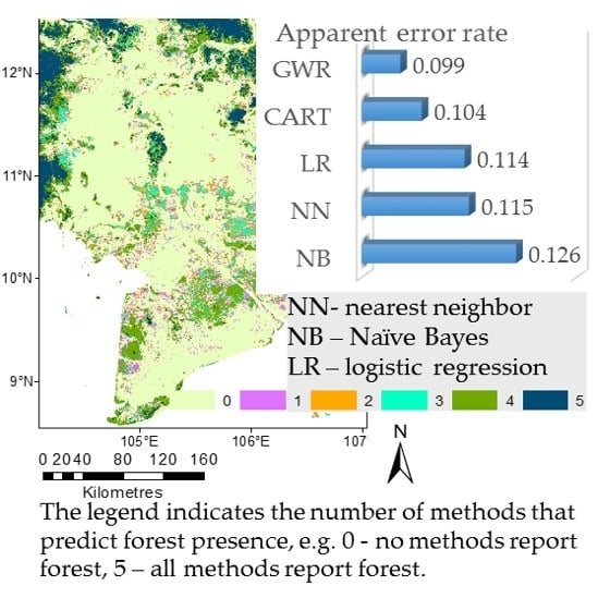
2. Data and Methods

2.1. Data Description

2.1.1. Input Layers

In this study, we use the same input datasets as Schepaschenko et al. [7] in the development of a global hybrid forest cover map, namely:
  • Global Land Cover Project 2000 (GLC2000) was generated by the Global Vegetation Monitoring Unit of the Joint Research Centre (JRC) of the European Commission with a network of international partners. It is a consistent global harmonized land cover database for the environmental reference year 2000 at a spatial resolution of 1 km. GLC2000 was produced using the VEGA 2000 dataset with 14 months of pre-processed daily global data acquired by the VEGETATION instrument on board the SPOT 4 satellite.
  • Global Land Cover by National Mapping Organisations 2003 was produced by the Global Mapping Project and organized by the International Steering Committee for Global Mapping (ISCGM). The product was generated in a raster format with a resolution of 1 km. It is organized into twenty land cover classes that are standardized by the Land Cover Classification System. As input data, 16-day composite Moderate Resolution Imaging Spectroradiometer (MODIS) data at a 1-km resolution for the year 2003 were used [28].
  • Global Land Cover Product 2005–2006 was produced by the European Space Agency (ESA) in collaboration with the JRC, EEA (European Environment Agency), FAO, UNEP (United Nations Environment Program), the GOFC-GOLD (Global Forest Cover-Global Land Dynamics) initiative and the International Geosphere-Biosphere Programme (IGBP). The product has a spatial resolution of 300 m. A detailed description is provided in [29].
  • Landsat-based continuous fields of tree cover 2000 (Vegetation Continuous Fields (VCF)) is a global product of 30-m resolution [30] and is available from the Global Land Cover Facility (GLCF) website (http://www.landcover.org).
  • MODIS land cover product 2001 was obtained through the online Data Pool at the NASA Land Processes Distributed Active Center (LP DAAC), United States Geological Survey (USGS)/Earth Resources Observation and Science (EROS) Centre (https://lpdaac.usgs.gov/data_access). The product was generated at a spatial resolution of 500 m at annual and biannual time steps. A detailed description of the dataset is given in [9].
  • The MODIS Vegetation Continuous Fields 2000 product is derived from the MODIS sensor, on-board the Terra and Aqua satellites, at a spatial resolution of 250 m [31].
  • Landsat-based tree cover 2000 is a global forest cover change product for the years 2000–2012 with a spatial resolution of 30 m and has been published by [2]. The product is based on Landsat imagery and has three components: forest cover 2000, forest gain 2000–2012 and forest loss per year.
  • The FAO forest map represents the tree canopy in 2010, with a spatial resolution of 250 m. It is freely available at http://www.fao.org/forestry/fra/80298/en/. Inputs to this product included MODIS VCF, maps of climatic zones, topography and water maps.
  • Regional maps that contain forest information. To account for regional and local specifications in forest cover, a number of regional land cover and land use maps were aggregated. These maps include: Congo Basin forest types map (Observatoire des forêts d'Afrique centrale (OFAC); http://www.observatoire-comifac.net/) that covers eight countries in Central Africa, i.e., Cameroon, Congo, Gabon, Burundi, Central African Republic, Equatorial Guinea, Democratic Republic of Congo and Rwanda [32]; Brazil PRODES (Programa Despoluição de Bacias Hidrográficas or Basin Restoration Program) forest mask 2000 [33]; Land Use of Australia 2005–2006 [34]; Pan-European Forest/Non-Forest Map 2000 (http://glcf.umiacs.umd.edu/data/landsat/); the National Land Cover Database 2006 (NLCD 2006) for the United States (available at http://www.mrlc.gov/nlcd06_data.php); land cover of Russia 2005 [14]; forest mask for European Russia 2000 [35].
These datasets originally have different resolutions from 30 m–1 km. These products with different resolutions are usually used for different purposes. For example, in many cases, users who want to use these data as inputs to their models do not require data at high resolution because the majority of input model variables are available at a regional level (e.g., IMPACT (International Model for Policy Analysis of Agricultural Commodities and Trade) provides results at the subnational level, the GLOBIOM (Global Biosphere Management Model) model operates at a 0.5 degree level, etc. [36]). For this reason, high or medium resolution data are first aggregated to a coarser grid. The products at a higher resolution are used for more in-depth local analyses, e.g., forest management in a certain forest enterprise. In this study, the datasets have been resampled to a 1-km grid, applying a set of aggregation rules that have been outlined previously in [7]. The input datasets have been pre-processed in two steps: (1) conversion of land cover classes to the probability of forest presence and forest cover according to the FAO definition; (2) aggregation of high resolution products to a 1-km resolution. The description of the aggregation process is provided in Appendix A.
All nine input layers are listed in Table 1.

2.1.2. Crowdsourced Data from Geo-Wiki

Crowdsourced data on forest cover were collected through the Geo-Wiki project [26], which aims at validating, correcting and enhancing land cover products [23,37,38]. Over numerous campaigns, volunteers have been asked to visually estimate land cover visible in cells of a grid overlaid onto very high resolution Google Earth imagery. The detailed description of the collection of data through Geo-Wiki is provided in [7]. Other examples of Geo-Wiki campaigns are given in [39,40]. The 1-km grid of the GLC2000 was used as the basis for the output map and, thus, a training dataset was compiled as a sub-sample from the various crowdsourced data campaigns where 1-km data were collected. The final training dataset contained 20,046 pixels of land cover information (presence/absence of forest) from around the globe. Figure 1 demonstrates the distribution of the training data points.
Geo-wiki data have been collected for the year 2000. Google Earth images were not always available for 2000, and therefore, we assume that: (1) for the pixels that are covered by forest, there is no difference, because, e.g., forest in 2005 has been a forest in 2000; (2) there was no forest loss where pixels are not covered by forest.

2.2. Methods

For building a hybrid forest map, the probability of forest presence in each grid cell was estimated using several methods detailed below. The overall idea is to benefit from the correlation between global forest cover datasets and the crowdsourced data. The crowdsourced data from Geo-Wiki are assumed to represent the ground-truth about forest absence/presence (dependent variable) while the input land/forest cover datasets are treated as independent variables. An overview of the methods compared is provided below.

2.2.1. Nearest Neighbour

Nearest neighbour (NN) is one of the simplest non-parametric methods used in a variety of applications. It uses the mean (for continuous) or mode (for categorical) of the variable of interest over the predefined neighbourhood as the estimator [41]. Despite its simplicity, when applied, it usually provides good final results. A general introduction to the method can be found in the book by Hastie, Tibshirani and Friedman [42].

2.2.2. Naive Bayes Classifier

The naive Bayes classifier (NB) is based on the well-known Bayesian theorem and can often outperform more sophisticated methods. It assumes that the inputs are conditionally independent in each class and uses the inverse probability formula to produce the likeliest category estimate [42,43]. The predictors are assumed to be independent. It is commonly implemented for classification tasks, including land cover classification [17]. Prior probabilities are very often chosen from proportions of each class in the training dataset, as implemented here in this study.

2.2.3. Logistic Regression Models

Logistic regression is another commonly-used classification method and is a generalised linear model employed when the response variable is binary. We tested logistic regression and geographically-weighted logistic regression (GWR): (1) ordinary logistic regression (LR) was used to generate a global equation to predict the probability of the presence of forest cover in a grid at the global level; (2) GWR estimates model parameters at each geographical location by using a distance weighted kernel, so that the observations closer to the studied location have more influence on the parameter estimates than the observations further away [44]. GWR was developed by Brunsdon et al. [45] as a spatial statistical method that allows regression parameters to vary over space. GWR has since been used in many different applications, e.g., in epidemiological studies [46], in the evaluation of net primary productivity in forests [47], in map accuracy assessment [38], in developing hybrid land cover maps [6,7], etc. The size of the bandwidth of GWR is usually optimized by cross-validation. We included ordinary logistic regression in this study to see the effect of the spatial component on the accuracy of the final result. The input data required for GWR are the coordinates of the centre of each pixel where the resolution and geometry should be the same as the final grid, and information on either the presence/absence of a particular land cover class or the percentage of a particular land cover type in the pixel. For all other methods, spatial information is not necessary, i.e., the coordinates of the pixel centre are not required.

2.2.4. Classification and Regression Trees

Tree-based methods are conceptually simple yet powerful techniques that partition the predictor space into a set of rectangles and then fit a simple model to each one. Regression trees are used for continuous responses, whereas classification trees are used for categorical ones. Classification and regression trees are referred to by the acronym CART and have been used in a variety of applications from ecological to medical tasks [20], e.g., for modelling tree species distribution [48], assessing risks of mortality from heart failure [49], etc.

2.3. Criteria for Comparison

The methods have been applied with two different types of input data: (1) binary forest presence/absence; (2) the percentage of forest cover within a grid cell. Both types of data have been extracted from the input land cover datasets (already aggregated) according to the forest-related class definitions; see [7]. We implemented the following statistical measures as criteria to compare the performance of the methods:
  • Apparent error rate, which is the proportion of incorrect predictions [50]. It is calculated by dividing the number of incorrectly classified data points by the overall number of data points.
  • Sensitivity, i.e., the proportion of true positives, and specificity, i.e., the proportion of true negatives, which are often used in medical classification problems [42].
  • Computational time (in seconds), which is the CPU (central processing unit of the computer) time required to run the methods.
The above criteria were applied to assess the candidate methods not only in terms of fit, but also in terms of predictive performance. For the latter purpose, a 10-fold cross-validation was performed (see [42] for more details).
All of the above methods were implemented using the R (Version 3.2.1) environment for statistical computing (R Core Team 2014). Maps of forest probabilities were converted to forest presence/absence maps by applying a threshold of 50%, following the example of the usage of logistic regression models in [51]. The apparent error rates of the different methods were found to be the smallest for a threshold of 50%.
We used the following R packages:

3. Results

3.1. Binary Presence/Absence of Forest Cover

The estimates of sensitivity, specificity and apparent error rate are summarized in Table 2. Sensitivity and specificity analysis shows that the non-forested areas are identified with more precision by GWR than by the other methods.
To test the statistical significance of the differences in apparent error rates, we applied the pairwise McNemar’s test [52]. The results, shown in Table 2 and Table 3, indicate that the lowest apparent error rate was obtained by GWR, and it is statistically-significantly different than the apparent error rates for the other four methods (p = 0.001). Furthermore, LR is statistically-significantly lower than NB, but otherwise, the four methods (NN, CART, NB and LR) appear to perform fairly similarly.
The input datasets spatially differ from each other, and it is not known which map is correct in the disagreement areas. For a more detailed analysis, we split the training datasets into subsets by “forest score”, which we define here as the number of land cover products that recognize forest presence in a pixel. Since there are nine forest cover products used in the analysis, the forest score will vary from 0–9. Figure 2a illustrates the apparent error rate by forest score. When most of the products agree either on forest presence (forest score close to one) or on forest absence (forest score close to zero), all of the methods show approximately the same accuracy. Only in high disagreement areas does GWR perform noticeably better than the other methods.
Table 4 presents a list of “forest scores” where the differences between apparent error rates are statistically significant at a 0.1% confidence level. At both ends of the forest score spectrum, the estimates of different methods are almost the same, i.e., the apparent error rates are very small when all of the products agree. GWR performs statistically-significantly better in high disagreement areas (particularly, forest score four) while NN and BN do not perform very well in disagreement areas.
There is a difference between predicting forests where no forest is present versus not predicting forest cover that is present in reality. To illustrate this, we selected points of high disagreement, i.e., “forest score” four, from the training datasets and plotted the corresponding estimates of sensitivity and specificity for these combined forest scores in Figure 2b. We only selected points of “forest score four” because in other areas, the methods perform almost the same. Figure 2b shows differentiation between sensitivity (correctly identifying the presence of forest) and specificity (correctly identifying the absence of forest). While the sensitivity is very high for all of the methods, the specificity is generally low. GWR performs better in correctly identifying the absence of forest than the other four methods. NB clearly overestimates the presence of forest because the sensitivity is close to one and the specificity is very low. We cannot make such a clear conclusion for other methods, because high sensitivity is followed by relatively low specificity.

3.2. Percentage of Forest Cover in a Grid Cell as Input Data

We carried out the same analysis to compare the methods using data on the percentage of forest cover in a grid cell. Table 5 summarizes the estimates of apparent error rate, sensitivity and specificity. Again, GWR appears to perform better than the other methods, but only slightly better than CART. The results of McNemar’s test on the statistical significance of differences are presented in Table 6. The difference between the apparent error rates of NN and LR is the only one that is not significant.
Figure 3a illustrates the apparent error rate for different forest scores. In general, the patterns are similar to those shown in Figure 2 (for the case of binary input data). Figure 3b shows the combined sensitivity and specificity estimates for forest scores four and five. As with the binary data, the sensitivity is observed to be high for all of the methods, while the specificity is very low, and GWR once again performs better in correctly identifying the absence of forest compared to the other four methods. NB overestimates the presence of forest once again. Table 7 shows “forest scores” for every pair of methods for which the difference in apparent error rate is statistically significant at a 0.1% confidence level.
Through the application of the methods, we generated five forest maps for the percentage of input data. These maps differ spatially from each other when compared. To illustrate these differences, we used an approach similar to the forest score, but applied this to the five methods. Thus, when all methods report the absence of forest, the method score is zero, while five represents the situation where all methods report forest cover. Figure 4 shows a combination of all five maps by method score. Although the analysis of the apparent error, sensitivity and specificity demonstrates that large forests, as well as large unforested areas are well recognized by all of the methods, in the territories with high land cover fragmentation, the results vary considerably, as shown in Figure 4.

4. Discussion

In this study, we have applied a variety of statistical methods to combine nine different forest cover maps with crowdsourced data from Geo-Wiki to produce a single hybrid forest cover map of high accuracy. The results show that using the percentage of forest cover (Section 3.1, first experiment) rather than simple dichotomous presence/absence of forest cover (
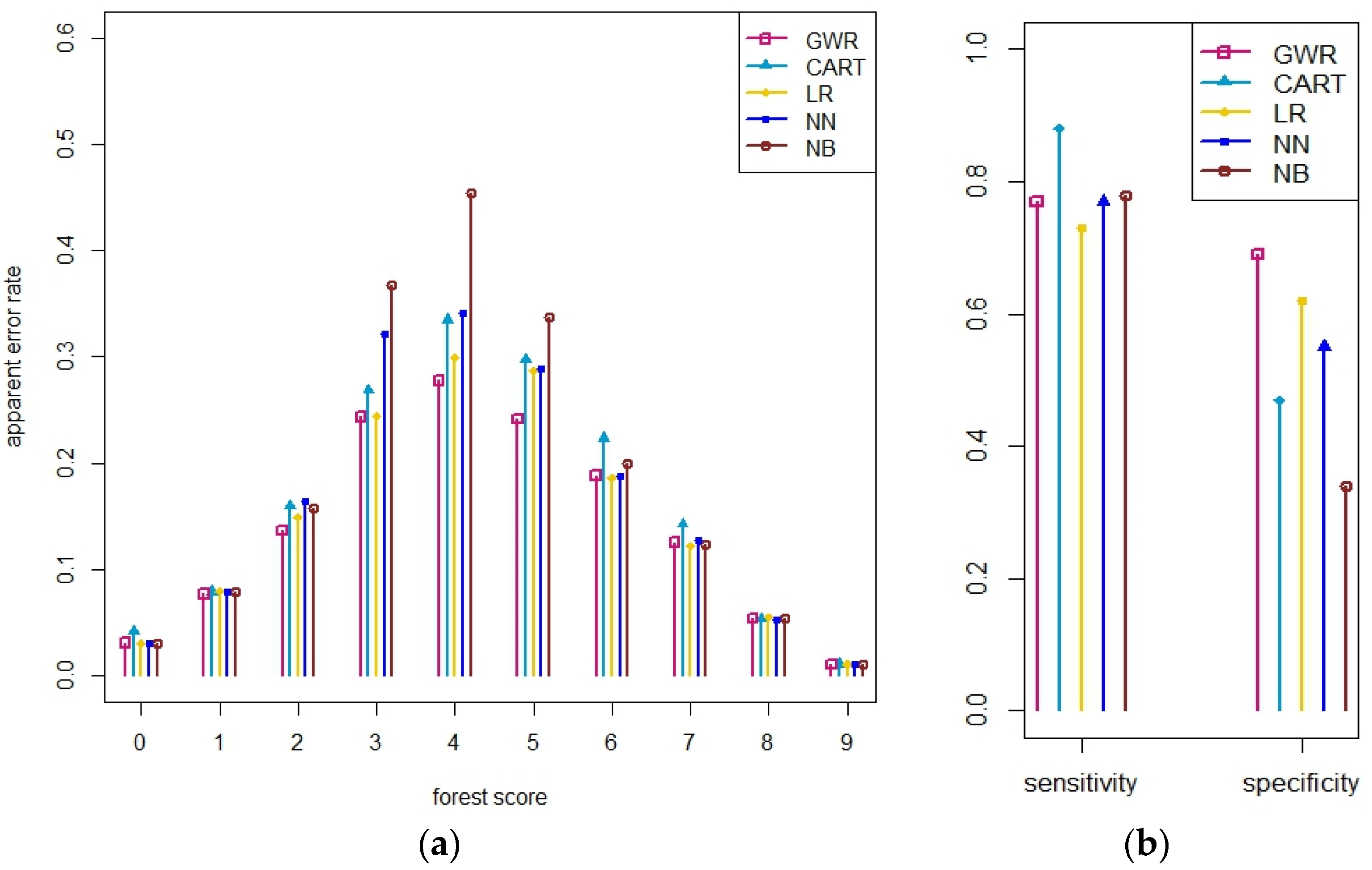
Section 3.2, second experiment) as the input results in a more accurate hybrid map. We also show that for areas with high disagreement among input maps, all of the methods have high sensitivity and low specificity, but that NB considerably overestimates forest.

4.1. Performance of the Methods

In this study, the NN and the NB methods have not performed well in comparison with other, parametric methods. One of the possible reasons for this is the fact that the training dataset does not adequately represent all possible combinations of the product inputs. The crowdsourced data from Geo-Wiki campaigns were collected to capture a wide range of land cover information that could be further used in different applications. This sample was not originally chosen based on the combinations of input layers. In this study, we wanted to show which of the methods extracts the maximum information available from the crowdsourced data and the input maps. Therefore, NN and NB are not recommended here. However, when more crowdsourced information is acquired in the future, they may prove to be more useful. Alternatively, if a sampling design was implemented specifically for these approaches, they may also perform better.
In general, the CART methods and ordinary logistic regression provided good results for both the binary input data, as well as for the continuous data. In the second experiment, where logistic regression was used, the performance is slightly better. Both methods are easy to implement using widely available statistical software (e.g., packages in R). A recent study that examined different types of data fusion methods, referred to in the paper as geographical stacking [25], showed that classification trees produced the best results when fusing different land cover datasets together, although the authors did not compare the methods with GWR.
By implementing NB for binary data, the method performed poorly for percentage input data in the areas of high disagreement, i.e., when half of the input products identified the presence of forest while the other indicated absence. There have been many studies undertaken to examine the performance of this method [53,54,55]; despite the assumption of the independence of the inputs, all of the studies showed that it gave good results in practice. However, this method still requires a deeper understanding of the data characteristics that affect its performance [53].
In general, GWR performed marginally better than the other methods, but it is in areas with high disagreement between the input datasets that the results of the prediction by GWR were found to be much more accurate. One of the advantages of this method is that the estimates of the model coefficients vary in space. From this, we can conclude that GWR provides the best results for the prediction of land cover classes through combining different data sources. This gain in accuracy has a trade-off in that it is more computationally intensive than the other methods tested. Moreover, it is important to mention that GWR is not statistically proven as a method for the analysis of nonstationary data. Wheeler and Tiefelsdorf [56] state that multicollinearities and pairwise correlations between sets of local coefficients do not provide appropriate model results. However, the method needs a more detailed study of its implementation for solving particular tasks, e.g., in the development of hybrid land cover maps.
We have also looked at the performance of the methods with different inputs to understand if the maps from different time periods, in particular the FAO map, decrease the performance of the final results. At the global level, there is no statistically-significant difference in the results when the FAO map is excluded. One of the reasons for this is that the apparent error rate of the forest products is higher than the relative change of forest area over time.

4.2. Accuracy Trade-Off

Table 8 presents the apparent error estimates of the input forest datasets. Some fusion methods were not able to outperform the accuracy of the individual input datasets. For example, NN and NB did not produce a map that is more accurate than Hansen’s tree cover (TC). However, the GWR resulted in improvements in forest map accuracy of around 2% compared to the most accurate input dataset of Hansen’s TC.
All of the differences in apparent error rates are statistically significant with high p-values equal to 0.001. Although the gain in accuracy is small, 1% of a land cover map is approximately 150 million hectares, which is a substantially-sized area, e.g., to place this in context, the area of Mongolia is around 155 million hectares In comparison with Hansen’s TC, a hybrid map better captures 2% of the land cover or approximately 300 M ha. These are territories that are very often found in the borders of forest land and where there are classification errors in the products (e.g., Hansen’s TC very often confuses wetlands with forest areas).
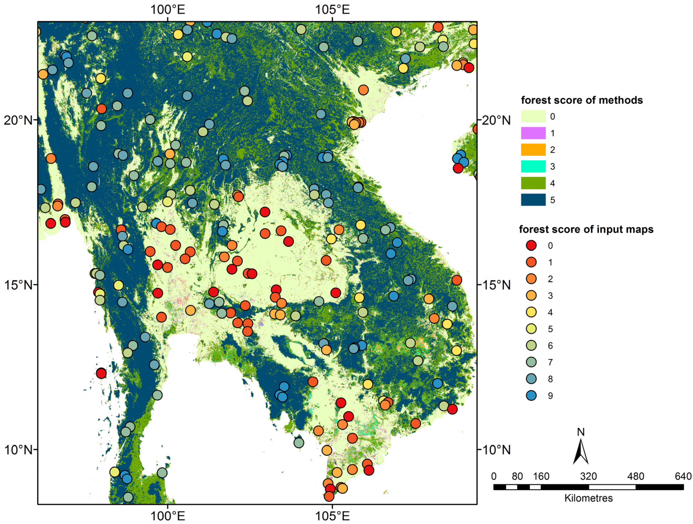
The results of comparing the methods show that for countries or bioclimatic zones where fragmentation of landscape structure is not high, in other words, the agreement areas of the input maps, there is little difference regarding which method to apply, e.g., tropical countries with rainforest. For regions with more complex landscape structures (e.g., Tanzania, Brazil), it is desirable to implement spatially-explicit methods (e.g., GWR) to develop a hybrid land cover map. As input data for these methods, it is crucial to collect as much training data of high quality as possible.
The geographically-weighted kernel used in GWR can also be implemented with other methods, including NB, CART and NN. With an increase in the amount of crowdsourced data or ground truth data and the development of new corresponding R packages, it will be interesting to compare the performance of spatially-explicit methods for building a hybrid land cover map. These will be the subject of further research.
In the paper on the development of a hybrid forest map for 2000 [7], the authors have applied GWR for the integration of crowdsourced data and land cover products. However, the authors did not undertake a comparative analysis of the performance of other methods for solving this task. The results of our study are valuable because they show that the difference in implementing GWR and other data fusion methods is small. However, the improvements from GWR were shown to be statistically significant.
The results of the study have important practical implications for building land cover maps of different land cover types. As new land cover products appear, it is always possible to build a hybrid land cover map by applying one of the data fusion methods outlined in the paper.

5. Conclusions

This paper presents a comparison of selected data fusion methods in predicting forest cover by integrating land cover datasets and crowdsourced data from Geo-Wiki. The results have shown that continuous data (percentage of land cover classes in a pixel) are preferable to binary data as the results are improved. Of the methods tested, GWR was shown to be the best fusion method for predicting the presence/absence of forest in terms of accuracy. This was especially true in areas with high disagreement among the input data sources. The CART and ordinary logistic regression were found to be the second best in terms of prediction accuracy. In practice, for the regions with homogeneous landscapes, it matters very little which method is chosen. However, for territories with highly fragmented landscapes, we recommend implementing a spatially-explicit method, e.g., GWR, as a data fusion method for producing hybrid land cover maps. GWR, as any other spatially-explicit method, is more demanding in terms of computing resources than the other methods, but we would argue that the increase in accuracy, albeit small overall, is worth the effort.

Acknowledgments

The work was supported by Marie Curie individual Grant FP7-MC-IIF: SIFCAS (Spatially integrated forest carbon accounting system) Project No. 627481 and the EU FP7-funded ERC grant Crowdland (No. 617754).

Author Contributions

All of the authors contributed to the discussion of the results, as well as to the writing of the manuscript. Myroslava Lesiv wrote the draft of the paper and conducted the numerical experiments of the methods, particularly GWR. Elena Moltchanova prepared R scripts for implementing the methods (NN, BN and CART) and contributed to the discussion of the results. Dmitry Schepaschenko designed the study and contributed in the writing and editing of the paper. Linda See participated in the discussions and also edited the paper. Anatoly Shvidenko, Steffen Fritz and Alex Comber helped in paper edits.

Conflicts of Interest

The authors declare no conflict of interest.

Appendix A. Supplementary Material on the Preparation of Input Datasets

The input land cover maps have been pre-processed via the following two steps: (1) conversion of land cover classes to the probability of forest presence and forest cover according to the FAO definition [27]; (2) aggregation of high resolution products to a 1-km resolution.
Step 1. Table A1 summarizes the set of rules applied to identify forest presence/absence and forest percentage in correspondence with FAO’s forest definition. For the tree cover products (e.g., FAO’s forest map, Hansen’s TC), the threshold of 10% was applied.
Table A1. Conversion of land cover classes to forest presence probability and forest cover. Source: [7].
Land Cover DefinitionCorrespondence to FAO Forest DefinitionAverage Forest Cover, %
Land Cover ClassTree Cover, %Forest Cover, %
GLC2000
Closed forest40–10080–100190
Tree cover, closed or open15–10080–100190
Open forest15–4080–100190
Degraded forest40–7080–100190
Forest plantations40–10080–100190
Mosaic: Forest/savannah40–7080–100190
Mosaic: Tree cover/other natural vegetation15–7050–80165
Mosaic: Tree cover/cropland15–7050–80165
Mosaic: Cropland/tree cover/other natural vegetation10–4010–40120
Deciduous woodland15–7080–100190
Open woodland15–4080–100190
Tree cover, burnt0–8050–100175
GLCNMO
Forest40–10060–100180
Tree open15–4060–100180
MODIS land cover
Forest60–10060–100180
Woody savannahs30–6060–100180
Non-woody savannahs10–3060–100180
GlobCover
Forest, closed to open15–10070–100185
Forest, closed40–10070–100185
Forest, open15–4070–100185
Mosaic cropland (50%–70%)/vegetation (grassland/shrubland/forest) (20%–50%)0–400–400.2520
Mosaic vegetation (grassland/shrubland/forest) (50%–70%)/cropland (20%–50%)0–600–700.3535
Mosaic forest or shrubland (50%–70%)/grassland (20%–50%)0–700–700.535
Step 2. The high resolution products were aggregated to a 1-km resolution. For example, if any individual MODIS pixel had a correspondence of one, the probability of forest was one, since this exceeded the minimum requirement of 0.5 ha (see Figure A1 for an example). Similarly, for Landsat products, if at least six 30-m pixels had greater than 10% tree cover, which then exceeds 0.5 ha, the forest presence of the 1-km aggregated pixel would be one. For tree cover products, such as VCF, a threshold of 10% was applied, and the forest percentage of the aggregated 1-km pixel was calculated in the same way as for the other land cover products.
Figure A1. An example of aggregating tree cover data from MODIS VCF at 250-m resolution to 1 km and calculating the percentage of forest cover: (a) the original tree cover values at 250 m of MODIS VCF; (b) conversion to forest/non-forest based on tree cover values greater than 10% covering more than 0.5 ha; (c) the forest cover percentage aggregated to 1 km is then 50%, since half of the sub-pixels are covered by forest. Source: [7].
Remotesensing 08 00261 g005

References

  1. Global Climate Observing System. GCOS Essential Climate Variables. Available online: http://www.wmo.int/pages/prog/gcos/index.php?name=EssentialClimateVariables (accessed on 3 September 2013).
  2. Hansen, M.C.; Potapov, P.V.; Moore, R.; Hancher, M.; Turubanova, S.A.; Tyukavina, A.; Thau, D.; Stehman, S.V.; Goetz, S.J.; Loveland, T.R.; et al. High-Resolution global maps of 21st-century forest cover change. Science 2013, 342, 850–853. [Google Scholar] [CrossRef] [PubMed]
  3. Jun, C.; Ban, Y.; Li, S. China: Open access to Earth land-cover map. Nature 2014, 514, 434–434. [Google Scholar] [CrossRef] [PubMed]
  4. Yu, L.; Wang, J.; Gong, P. Improving 30 m global land-cover map FROM-GLC with time series MODIS and auxiliary data sets: A segmentation-based approach. Int. J. Remote Sens. 2013, 34, 5851–5867. [Google Scholar] [CrossRef]
  5. Wulder, M.A.; Masek, J.G.; Cohen, W.B.; Loveland, T.R.; Woodcock, C.E. Opening the archive: How free data has enabled the science and monitoring promise of Landsat. Remote Sens. Environ. 2012, 122, 2–10. [Google Scholar] [CrossRef]
  6. See, L.; Schepaschenko, D.; Lesiv, M.; McCallum, I.; Fritz, S.; Comber, A.; Perger, C.; Schill, C.; Zhao, Y.; Maus, V.; et al. Building a hybrid land cover map with crowdsourcing and geographically weighted regression. ISPRS J. Photogramm. Remote Sens. 2015, 103, 48–56. [Google Scholar] [CrossRef] [Green Version]
  7. Schepaschenko, D.; See, L.; Lesiv, M.; McCallum, I.; Fritz, S.; Salk, C.; Moltchanova, E.; Perger, C.; Shchepashchenko, M.; Shvidenko, A.; et al. Development of a global hybrid forest mask through the synergy of remote sensing, crowdsourcing and FAO statistics. Remote Sens. Environ. 2015, 162, 208–220. [Google Scholar] [CrossRef]
  8. Fritz, S.; Bartholomé, E.; Belward, A.; Hartley, A.; Stibig, H.-J.; Eva, H.; Mayaux, P. Harmonisation, Mosaicing and Production of the Global Land Cover 2000 Database (Beta Version); Office for Official Publications of the European Communities: Luxembourg, 2003; p. 41. [Google Scholar]
  9. Friedl, M.A.; Sulla-Menashe, D.; Tan, B.; Schneider, A.; Ramankutty, N.; Sibley, A.; Huang, X. MODIS Collection 5 global land cover: Algorithm refinements and characterization of new datasets. Remote Sens. Environ. 2010, 114, 168–182. [Google Scholar] [CrossRef]
  10. Bicheron, P.; Defourny, P.; Brockmann, C.; Schouten, L.; Vancutsem, C.; Huc, M.; Bontemps, S.; Leroy, M.; Achard, F.; Herold, M.; et al. Globcover: Products Description and Validation Report; Medias France: Toulouse, France, 2008; p. 47. [Google Scholar]
  11. Fritz, S.; See, L.; McCallum, I.; Schill, C.; Obersteiner, M.; van der Velde, M.; Boettcher, H.; Havlík, P.; Achard, F. Highlighting continued uncertainty in global land cover maps for the user community. Environ. Res. Lett. 2011, 6, 044005. [Google Scholar] [CrossRef]
  12. Drusch, M.; Del Bello, U.; Carlier, S.; Colin, O.; Fernandez, V.; Gascon, F.; Hoersch, B.; Isola, C.; Laberinti, P.; Martimort, P.; et al. Sentinel-2: ESA’s optical high-resolution mission for GMES operational services. Sentin. Missions New Oppor. Sci. 2012, 120, 25–36. [Google Scholar] [CrossRef]
  13. Castanedo, F. A review of data fusion techniques. Sci. World J. 2013, 2013, 704504. [Google Scholar] [CrossRef] [PubMed]
  14. Schepaschenko, D.; McCallum, I.; Shvidenko, A.; Fritz, S.; Kraxner, F.; Obersteiner, M. A new hybrid land cover dataset for Russia: A methodology for integrating statistics, remote sensing and in-situ information. J. Land Use Sci. 2011, 6, 245–259. [Google Scholar] [CrossRef]
  15. Fritz, S.; You, L.; Bun, A.; See, L.; McCallum, I.; Schill, C.; Perger, C.; Liu, J.; Hansen, M.; Obersteiner, M. Cropland for sub-Saharan Africa: A synergistic approach using five land cover data sets. Geophys. Res. Lett. 2011, 38. [Google Scholar] [CrossRef]
  16. Song, X.-P.; Huang, C.; Feng, M.; Sexton, J.O.; Channan, S.; Townshend, J.R. Integrating global land cover products for improved forest cover characterization: An application in North America. Int. J. Digit. Earth 2014, 7, 1–16. [Google Scholar] [CrossRef]
  17. Li, W.; Zhang, C.; Willig, M.; Dey, D.; Wang, G.; You, L. Bayesian Markov Chain random field cosimulation for improving land cover classification accuracy. Math. Geosci. 2015, 47, 123–148. [Google Scholar] [CrossRef]
  18. Haapanen, R.; Ek, A.R.; Bauer, M.E.; Finley, A.O. Delineation of forest/nonforest land use classes using nearest neighbor methods. Remote Sens. Environ. 2004, 89, 265–271. [Google Scholar] [CrossRef]
  19. Meng, Q.; Cieszewski, C.J.; Madden, M.; Borders, B.E. K Nearest neighbor method for forest inventory using remote sensing data. GISci. Remote Sens. 2007, 44, 149–165. [Google Scholar] [CrossRef]
  20. De’ath, G.; Fabricius, K.E. Classification and regression trees: A powerful yet simple technique for ecological data analysis. Ecology 2000, 81, 3178–3192. [Google Scholar] [CrossRef]
  21. Dickinson, J.L.; Shirk, J.; Bonter, D.; Bonney, R.; Crain, R.L.; Martin, J.; Phillips, T.; Purcell, K. The current state of citizen science as a tool for ecological research and public engagement. Front. Ecol. Environ. 2012, 10, 291–297. [Google Scholar] [CrossRef]
  22. Clery, D. Galaxy Zoo volunteers share pain and glory of research. Science 2011, 333, 173–175. [Google Scholar] [CrossRef] [PubMed]
  23. Fonte, C.C.; Bastin, L.; See, L.; Foody, G.; Lupia, F. Usability of VGI for validation of land cover maps. Int. J. Geogr. Inf. Sci. 2015, 29, 1–23. [Google Scholar] [CrossRef]
  24. Caruana, R.; Niculescu-Mizil, A. An empirical comparison of supervised learning algorithms. In Proceedings of the 23rd International Conference on Machine Learning, Pittsburgh, PA, USA, 25–29 June 2006; pp. 161–168.
  25. Clinton, N.; Yu, L.; Gong, P. Geographic stacking: Decision fusion to increase global land cover map accuracy. Glob. Land Cover Mapp. Monit. 2015, 103, 57–65. [Google Scholar] [CrossRef]
  26. Fritz, S.; McCallum, I.; Schill, C.; Perger, C.; See, L.; Schepaschenko, D.; van der Velde, M.; Kraxner, F.; Obersteiner, M. Geo-Wiki: An online platform for improving global land cover. Environ. Model. Softw. 2012, 31, 110–123. [Google Scholar] [CrossRef]
  27. Food and Agriculture Organisation of the United Nations (FAO). Global Forest Resources Assessment 2010; FAO Forestry Paper 163; FAO: Rome, Italy, 2010. [Google Scholar]
  28. Tateishi, R.; Bayer, M.; Ghar, A.; Al-Bilbisi, H.; Tsendayush, J.; Shalaby, A.; Alimujiang, K.; Hoan, N.T.; Kobayashi, T.; Alsaaideh, B.; et al. A new global land cover map, GLCNMO. Int. Arch. Photogramm. Remote Sens. Spat. Inf. Sci. 2008, XXXVII, 1369–1372. [Google Scholar]
  29. Defourny, P.; Vancustem, C.; Bicheron, P.; Brockmann, C.; Nino, F.; Schouten, L.; Leroy, M. GLOBCOVER: A 300m global land cover product for 2005 using ENVISAT MERIS time series. In Proceedings of the ISPRS Commission VII Mid-Term Symposium: Remote Sensing: From Pixels to Processes, Enscede, The Netherlands, 8–11 May 2006.
  30. Sexton, J.O.; Song, X.-P.; Feng, M.; Noojipady, P.; Anand, A.; Huang, C.; Kim, D.-H.; Collins, K.M.; Channan, S.; DiMiceli, C.; et al. Global, 30-m resolution continuous fields of tree cover: Landsat-based rescaling of MODIS vegetation continuous fields with lidar-based estimates of error. Int. J. Digit. Earth 2013, 6, 427–448. [Google Scholar] [CrossRef]
  31. DiMiceli, C.M.; Carroll, M.L.; Sohlberg, R.A.; Huang, C.; Hansen, M.C.; Townshend, J.R.G. Annual Global Automated MODIS Vegetation Continuous Fields (MOD44B) at 250 m Spatial Resolution for Data Years Beginning Day 65, 2000–2010, Collection 5 Percent Tree Cover; University of Maryland: College Park, MD, USA, 2011. [Google Scholar]
  32. Verhegghen, A.; Mayaux, P.; De Wasseige, C.; Defourny, P. Mapping Congo Basin vegetation types from 300 m and 1 km multi-sensor time series for carbon stocks and forest areas estimation. Biogeosciences 2012, 9, 5061–5079. [Google Scholar] [CrossRef] [Green Version]
  33. Kempeneers, P.; Sedano, F.; Pekkarinen, A.; Seebach, L.; Strobl, P.; San-Miguel-Ayanz, J. Pan-European forest maps derived from optical satellite imagery. Earthzine 2012, 5, 390004. [Google Scholar]
  34. Australian Bureau of Agricultural and Resource Economics and Science. Guidelines for Land Use Mapping in Australia: Principles, Procedures and Definitions, 4th ed.Australian Bureau of Agricultural and Resource Economics and Science: Canberra, Australia, 2011.
  35. Potapov, P.; Turubanova, S.; Hansen, M.C. Regional-scale boreal forest cover and change mapping using Landsat data composites for European Russia. Remote Sens. Environ. 2011, 115, 548–561. [Google Scholar] [CrossRef]
  36. Nelson, G.C.; Valin, H.; Sands, R.D.; Havlík, P.; Ahammad, H.; Deryng, D.; Elliott, J.; Fujimori, S.; Hasegawa, T.; Heyhoe, E.; et al. Climate change effects on agriculture: Economic responses to biophysical shocks. Proc. Natl. Acad. Sci. USA 2014, 111, 3274–3279. [Google Scholar] [CrossRef] [PubMed] [Green Version]
  37. Comber, A.; See, L.; Fritz, S.; Van der Velde, M.; Perger, C.; Foody, G. Using control data to determine the reliability of volunteered geographic information about land cover. Int. J. Appl. Earth Obs. Geoinf. 2013, 23, 37–48. [Google Scholar] [CrossRef]
  38. Comber, A.; Fisher, P.; Brunsdon, C.; Khmag, A. Spatial analysis of remote sensing image classification accuracy. Remote Sens. Environ. 2012, 127, 237–246. [Google Scholar] [CrossRef]
  39. Fritz, S.; McCallum, I.; Schill, C.; Perger, C.; Grillmayer, R.; Achard, F.; Kraxner, F.; Obersteiner, M. Geo-Wiki.Org: The use of crowdsourcing to improve global land cover. Remote Sens. 2009, 1, 345–354. [Google Scholar] [CrossRef]
  40. See, L.; Fritz, S.; Thornton, P.; You, L.; Becker-Reshef, I.; Justice, C.O.; Leo, O.; Herrero, M. Building a Consolidated Community Global Cropland Map. Earthzine. Available online: http://www.earthzine.org/2012/01/24/building-a-consolidated-community-global-cropland-map/ (accessed on 23 April 2013).
  41. Efron, B.; Tibshirani, R.J. An Introduction to the Bootstrap; CRC Press: Boca Raton, FL, USA, 1994. [Google Scholar]
  42. Hastie, T.; Tibshirani, R.; Friedman, J. The Elements of Statistical Learning: Data Mining, Inference, and Prediction; Springer: New York, NY, USA, 2009; p. 745. [Google Scholar]
  43. Russell, S.J.; Norvig, P. Artificial Intelligence: A Modern Approach; Prentice Hall International Editions Series; Prentice Hall: Upper Saddle River, NJ, USA, 1995. [Google Scholar]
  44. Fotheringham, A.S.; Brunsdon, C.; Charlton, M. Geographically Weighted Regression: The Analysis of Spatially Varying Relationships; John Wiley & Sons: Chichester, UK, 2002. [Google Scholar]
  45. Brunsdon, C.; Fotheringham, S.; Charlton, M. Geographically weighted regression-modelling spatial non-stationarity. J. R. Stat. Soc. Ser. Stat. 1998, 47, 431–443. [Google Scholar] [CrossRef]
  46. Waller, L.A.; Gotway, C.A. Applied Spatial Statistics for Public Health Data; John Wiley & Sons, Inc.: Hoboken, NJ, USA, 2004; p. 520. [Google Scholar]
  47. Wang, Q.; Ni, J.; Tenhunen, J. Application of a geographically-weighted regression analysis to estimate net primary production of Chinese forest ecosystems. Glob. Ecol. Biogeogr. 2005, 14, 379–393. [Google Scholar] [CrossRef]
  48. Prasad, A.; Iverson, L.; Liaw, A. Newer classification and regression tree techniques: bagging and random forests for ecological prediction. Ecosystems 2006, 9, 181–199. [Google Scholar] [CrossRef]
  49. Fonarow, G.C.; Adams, K.F.; Abraham, W.T.; Yancy, C.W.; Boscardin, W. Risk stratification for in-hospital mortality in acutely decompensated heart failure: Classification and regression tree analysis. J. Am. Med. Assoc. 2005, 293, 572–580. [Google Scholar] [CrossRef] [PubMed]
  50. Martin, K.J.; Hirschberg, D.S. Small Sample Statistics for Classification Error Rates II: Confidence Intervals and Significance Tests; University of California: Irvine, USA, 1996. [Google Scholar]
  51. Pampel, F.C. Logistic Regression: A Primer; SAGE: London, UK, 2000. [Google Scholar]
  52. Foody, G.M. Thematic map comparison: Evaluating the statistical significance of differences in classification accuracy. Photogramm. Eng. Remote Sens. 2004, 70, 627–633. [Google Scholar] [CrossRef]
  53. Rish, I. An Empirical Study of the Naive Bayes Classifier; Computer Science; IBM Research Division, Thomas J. Watson Research Center: Yorktown Heights, NY, USA, 2015. [Google Scholar]
  54. Zhang, H. The Optimality of Naive Bayes. In Proceedings of the Seventeenth International Florida Artificial Intelligence Research Society Conference; AAAI (American Association for Artificial Intelligence) Press: Menlo Park, CA, USA, 2004; pp. 562–567. [Google Scholar]
  55. Schneider, K.-M. Techniques for improving the performance of naive bayes for text classification. In Proceedings of the 6th International Conference on Computational Linguistics and Intelligent Text Processing, Mexico City, Mexico, 13–19 February 2005; Springer-Verlag: Mexico City, Mexico, 2005; pp. 682–693. [Google Scholar]
  56. Wheeler, D.; Tiefelsdorf, M. Multicollinearity and correlation among local regression coefficients in geographically weighted regression. J. Geogr. Syst. 2005, 7, 161–187. [Google Scholar] [CrossRef]
Figure 1. Distribution of the training data points. The legend corresponds to a forest score, which is the number of input layers defining forest cover at the point locations (see Section 3.1 for more explanation).
Remotesensing 08 00261 g001
Figure 2. Binary response: forest presence/absence: (a) apparent error rate by forest score; (b) sensitivity and specificity estimated for the high disagreement area (“forest score” four).
Remotesensing 08 00261 g002
Figure 3. Percentage of forest in a grid: (a) apparent error rate by forest scores; (b) sensitivity and specificity estimated for the high disagreement areas (combined forest scores “four” and “five”).
Remotesensing 08 00261 g003
Figure 4. The agreement between the forest cover maps produced by the NN, NB, CART, LR and GWR methods. The “forest score of the methods” indicates the number of methods that predict forest presence, e.g., 0, no methods report forest; 5, all methods report forest. The coloured bubbles (the training dataset) correspond to the forest score according to the input maps (0, if no product reports forest; 9, if all of the products report forest).
Remotesensing 08 00261 g004
Table 1. List of input layers.
Input DatasetsAcronymYear of ReferenceResolutionLink to the Web Site
Global Land Cover Project 2000GLC200020001 kmhttp://bioval.jrc.ec.europa.eu/products/glc2000/products.php
Global Land Cover by National Mapping OrganisationsGLCNMO20031 kmhttp://www.iscgm.org/gm/glcnmo.html
Global Land Cover Product 2005–2006GlobCover2005300 mhttp://due.esrin.esa.int/globcover/
Landsat-based continuous fields of tree cover 2000Landsat VCF200030 mwww.landcover.org
MODIS land cover product 2001MCD12Q12001500 mhttps://lpdaac.usgs.gov/data_access
Landsat-based tree cover 2000Hansen’s TC200030 mhttp://earthenginepartners.appspot.com/science-2013-global-forest
MODIS Vegetation Continuous FieldsVCF2000250 mhttp://modis-land.gsfc.nasa.gov/vcc.html
The FAO forest mapFAO forest map2010250 mhttp://www.fao.org/forestry/fra/80298/en/
Regional productsRegional2000–20061 kmSee description above
Table 2. Binary data: apparent error rate, sensitivity and specificity. GWR, geographically-weighted regression.
MethodsApparent Error RateSensitivitySpecificity
NN0.1260.8210.919
CART0.1250.8440.902
NB0.1280.8150.921
LR0.1240.8280.917
GWR0.1150.8380.925
Table 3. McNemar’s test: p-values for the pairwise comparison of method performance in terms of apparent error rates.
MethodsCARTNBLRGWR
NN0.2680.2390.130<0.001
CART-0.0420.681<0.001
NB--<0.001<0.001
LR---<0.001
Table 4. McNemar’s test. Lists of “forest scores” for every pair of methods for which the difference in the apparent error rate is statistically significant.
CARTNBLRGWR
NN73; 75; 72; 4; 5
CART 3-2; 4
NB 32; 3; 4
LR 2; 4
Table 5. Continuous data: apparent error rate, sensitivity and sensitivity estimates.
MethodsApparent Error RateSensitivitySpecificity
NN0.1150.8760.893
CART0.1040.9090.884
NB0.1260.8410.903
LR0.1140.8450.921
GWR0.0990.8700.927
Table 6. McNemar’s test: p-values for each pair of methods.
CARTNBLRGWR
NN<0.001<0.0010.830<0.001
CART-<0.001<0.0010.004
NB--<0.001<0.001
LR---<0.001
Table 7. McNemar’s test. Lists of “forest scores” for every pair of methods for which the difference in the apparent error rate is statistically significant.
MethodsCARTNBLRGWR
NN0; 60; 3; 40; 3; 60; 2; 4; 5
CART 3; 4; 535
NB 3; 42; 3; 4; 5
LR 2; 3; 4; 5
Table 8. Apparent error rate estimates of the input forest datasets.
Input Forest DatasetsTraining Dataset
FAO forest map0.14
GLC20000.23
GLCNMO0.24
GlobCover0.24
Landsat VCF0.15
Modis land cover0.20
Regional products0.21
Modis VCF0.26
Hansen’s TC0.12
GWR (percentage data)0.10

