Article

Anatomy of Subsidence in Tianjin from Time Series InSAR

1
Key Laboratory for Geo-Environment Monitoring of Coastal Zone of the National Administration of Surveying, Mapping and GeoInformation & Shenzhen Key Laboratory of Spatial Smart Sensing and Services, Shenzhen University, Shenzhen 518060, China
2
College of Information Engineering, Shenzhen University, Shenzhen 518060, China
3
Center for Observation & Modeling of Earthquakes, Volcanoes & Tectonics (COMET), School of Civil Engineering and Geosciences, Newcastle University, Newcastle upon Tyne, Tyne and Wear NE1 7RU, UK
4
School of Geographical & Earth Science, University of Glasgow, Scotland G12 8QQ, UK
5
Department of Surveying Engineering, Southwest Jiaotong University, Chengdu 610031, China
*
Author to whom correspondence should be addressed.
Submission received: 15 December 2015 / Revised: 10 March 2016 / Accepted: 14 March 2016 / Published: 22 March 2016
(This article belongs to the Special Issue Earth Observations for Geohazards)

Abstract

:
Groundwater is a major source of fresh water in Tianjin Municipality, China. The average rate of groundwater extraction in this area for the last 20 years fluctuates between 0.6 and 0.8 billion cubic meters per year. As a result, significant subsidence has been observed in Tianjin. In this study, C-band Envisat (Environmental Satellite) ASAR (Advanced Synthetic Aperture Radar) images and L-band ALOS (Advanced Land Observing Satellite) PALSAR (Phased Array type L-band Synthetic Aperture Radar) data were employed to recover the Earth’s surface evolution during the period between 2007 and 2009 using InSAR time series techniques. Similar subsidence patterns can be observed in the overlapping area of the ASAR and PALSAR mean velocity maps with a maximum radar line of sight rate of ~170 mm·year−1. The west subsidence is modeled for ground water volume change using Mogi source array. Geological control by major faults on the east subsidence is analyzed. Storage coefficient of the east subsidence is estimated by InSAR displacements and temporal pattern of water level changes. InSAR has proven a useful tool for subsidence monitoring and displacement interpretation associated with underground water usage.

Graphical Abstract

1. Introduction

Subsidence caused by groundwater extraction is a worldwide problem [1,2,3]. Estimated subsidence rates range up to several hundred mm per year, highlighting the importance of continuous displacement mapping. With great demand for fresh water and a limited river water resource, ground water use seems inevitable for Tianjin City (Figure 1a), which has a population of 12.93 million and is currently growing at 2.6% per year till 2010 [4]. The maximum pumping rate recorded was in 1981 with the annual rate of 1.2 × 10⁹ m3. The annual rates from 1981 to 2007 are in the range 0.6–0.8 × 10⁹ m3·year−1 (Figure 1b) [5]. As a consequence of this sustained high level of abstraction, an overall drop in the water table has been observed in Tianjin. Water extraction has increasingly been from deeper underground [6]. This extensive use of ground water could account for the subsidence in Tianjin, which has been observed since 1959. The subsidence can be divided into three different stages: slow subsidence at 50 mm·year−1 from 1959 to 1977, accelerating subsidence from 1978 to 1982 at 100 mm·year−1 and attenuating subsidence at 20–30 mm·year−1 from 1983 to 1997 [7]. The maximum total subsidence from 1959 to 2008 has reached 3.2 meters [5]. Locally, higher rates have been recorded: in the 1980s, the maximum subsidence rate is given as 250 mm·year−1 in Tianjin [6]. The current subsidence rate has been estimated as 8–56 mm·year−1 [6] and 30–40 mm·year−1 [5].
InSAR (Interferometric Synthetic Aperture Radar) has been used to map subsidence due to groundwater extraction in Tianjin [8,9,10] and other areas like Shanghai [11], Mekong delta [12], Ganges-Brahmaputra delta [13], Iran [14,15,16,17], Reykjanes Peninsula [18] and so on. In this study, an InSAR time series technique is also used to recover the surface displacement field over the urban area of Tianjin between 2007 and 2009. The patterns of observed subsidence are then interpreted in details and modeled. Subsidence is concentrated in particular areas of the city, and these subsidence centers are analyzed in terms of their geological controls and association with groundwater levels. The effects of groundwater volume changes on surface displacement are investigated for one subsidence center through inverse modeling of InSAR derived subsidence.

2. Geological Background

2.1. Tectonic Divisions

Tianjin Municipality is located 130 km southeast of Beijing and is on the western shore of Bohai Gulf. Tianjin lies on the North China Plain (NCP), also known as Huabei Plain. The NCP is dominated by Haihe and Cangdong fault systems (Figure 1a). The NNE-SSW oriented alignment of Cangdong fault, Tianjin fault, and the Paleogene lacuna, forms a horst-graben structure, which is transversely cut by WNW-ESE aligned faults including Baodi, Hangu, and Haihe faults [24].
In summary, Tianjin is separated by Baodi Fault into the northern Yanshan Folded Belt and the southern Bohai Bay Basin. The Bohai Bay basin contains three tectonic divisions: Jizhong depression, Cangxian uplift, and Huanghua depression. Paleogene lacuna separates Jizhong depression and Cangxian uplift. Cangdong fault separates the Cangxian uplift and the Huanghua depression [25].

2.2. Sediments

The stratigraphy in the Bohai Bay Basin is summarized in Figure 1c. The Bohai Bay Basin is a tectonically subsiding region filled with continental Tertiary and Quaternary sediments [21]. The Quaternary and Tertiary sediments and aquifer system range in thickness from less than 1000 m in the Cangxian uplift [22] to 1200–9000 m in the Jizhong depression, and 900–5000 m in the Huanghua depression [20].

2.3. Hydrogeological Conditions

The ground water system in Tianjin has three main aquifers, the Quaternary, Tertiary and Lower Paleozoic-Sinian aquifers [22]. Above the depth of 700 m in Tianjin, the ground water system can be sub-divided into six aquifer layers (Table 1) [26]. Thickness of Aquifers I to V are in the range of 40–60, 25–60, 30–55, 30–50, and 20–30 m, respectively [6]. Aquifer II is in an over consolidated late Pleistocene strata and Aquifer III is in a normally consolidated middle Pleistocene strata. In Tanggu district of Tianjin, even though aquifer II and III account for 46% and 24% of ground water exploitation, respectively, Aquifer III is the greatest deformation contribution source [7]. Layers between 136 m and 300 m in depth account for more than 65% of subsidence by extensometer observation in Tanggu district of Tianjin [7].
The ground water extracted from a depth greater than 300 meters is mainly used for geothermal exchange. The Tianjin geothermal field covers approximately 11,000 km2 [22]. The horst where Tianjin is located is the most productive geothermal field and the highest measured geothermal gradients are found here. More than 200 geothermal wells, of which 10–15 are injection wells, are producing waters from 30 °C to boiling for room heating. Shallow geothermal wells range from 300 m in Quaternary formations to 600 m in Tertiary formations for lower temperatures. Deep wells can reach up to 2600 m in the Tertiary formation [22].

3. Data and Methods

3.1. Data

In order to investigate the subsidence in Tianjin, an InSAR (Interferometric Synthetic Aperture Radar) method is used [28,29], exploring C-band Envisat-ASAR data from European Space Agency (ESA) and L-band ALOS-PALSAR data from Japan Aerospace Exploration Agency (JAXA). ASAR C band images (Table 2) are retrieved with a wavelength of 56 mm compared with PALSAR L band images (Table 3) of 236 mm. The radar line of sight look angles are 23 and 34 degrees off nadir for ASAR and PALSAR, respectively, which means a different sensitivity towards the vertical deformation. The azimuth angles are 166 and 13 degrees counter clockwise from north for ASAR and PALSAR, respectively.

3.2. Methods

Single look complex image was generated using ROI_PAC [28]. Interferograms were generated using Doris [30]. SRTM (NASA’s Shuttle Radar Topography Mission) with a 3 arc-second resolution was used for topography removal [31]. The StaMPS (Stanford Method for Persistent Scatterers) software was used to process the images using Persistent Scattering (PS) methods inside the package [32,33].
In contrast to most other PS methods, StaMPS uses phase spatial correlation to identify PS pixels instead of amplitude analysis [30,34,35]. The advantage of this strategy is the capability to detect persistent scattering (PS)/slowly decorrelating filtered phase (SDFP) pixels with low amplitude, which is often the case in natural terrains. The probability for a pixel to be PS/SDFP is estimated through phase analysis, which is successively refined in a series of iterations. Without any prior assumption about the temporal nature of ground deformation, StaMPS relies on the spatial correlation of deformation rather than any assumption of the temporal dependence of deformation [36].
For selected PS points, the two dimensional phases are still modulo 2π. Phase unwrapping is therefore implemented in order to derive continuous displacement fields. On each interferogram, phase unwrapping is implemented using the SNAPHU (Statistical-Cost, Network-Flow Algorithm for Phase Unwrapping) algorithm [37]. SNAPHU is a statistical-cost network flow algorithm. The algorithm aims to compute the most likely unwrapped solution with maximum posterior probability estimation given the observable input data.
The topography of the NCP (North China Plain) is quite gentle because it is formed in a coastal area by sediment aggradations. Large DEM errors are not expected here. The look angle error is estimated in time series using perpendicular baselines of each scene [32].
The atmospheric effects exhibit spatially correlated pattern. Deformation pattern are also spatially correlated. However, displacement usually stays in the same area while the atmospheric phase screen (APS) pattern is variable from one image to another. For a single pixel, the deformation should be continuous in time, APS will cause unexpected signal in time series. The APS can be estimated according to its different spatial and temporal nature from displacement. The master atmospheric effect and orbital error is estimated by its presence in every interferogram. The slave atmospheric effect and orbital error is estimated by temporal high pass and spatial low pass filtering [32]. As a flood plain, our research area in NCP shows gentle topography with height ranges between −16 and +68 m. As a result, the topography dependent APS [38,39,40], which could stay in the same area and be misunderstood as displacement, are believed to be small. Long-wavelength atmospheric effects and imprecise orbit errors were reduced by a planar phase gradient.

4. Results

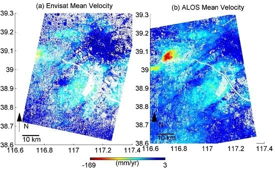
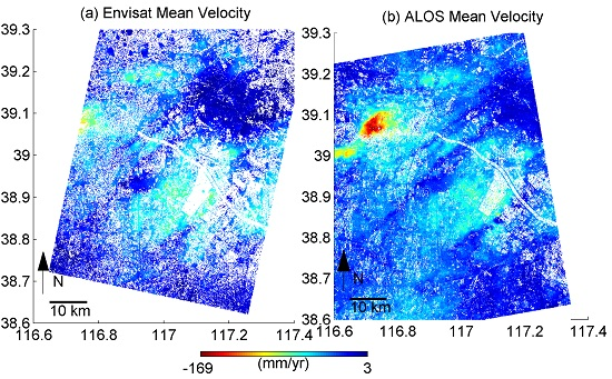
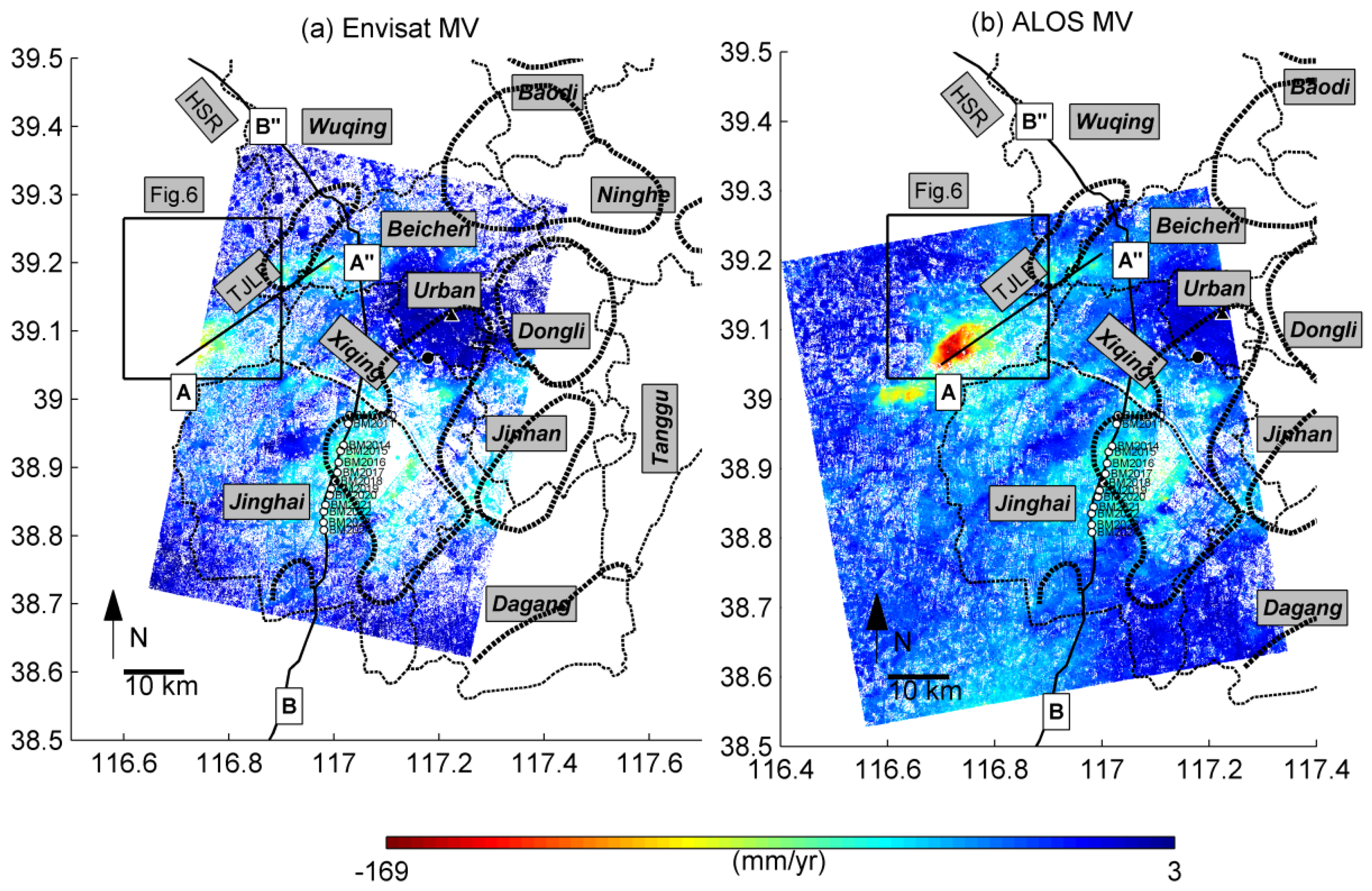
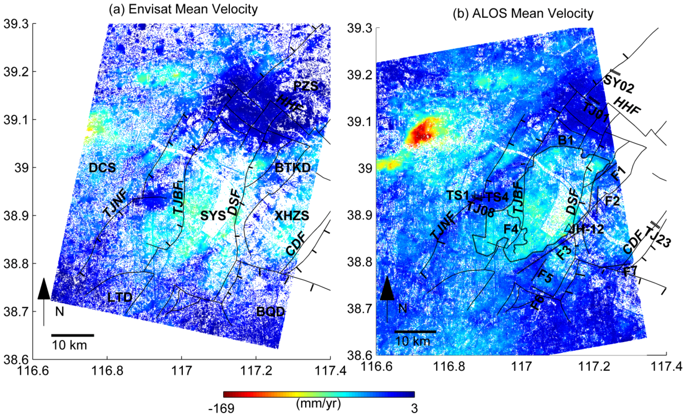
4.1. Mean Velocities from ALOS and Envisat

The mean phase values of each image are firstly used as the reference phase in time series analysis because no ground truth data are available. The area with obvious uplift displacements on the resulting mean velocity map was then chosen as the reference area (small triangle in Figure 2). The Envisat and ALOS mean velocity rates are not uniform across the study area with similar pattern of individual subsidence zones on both maps. Two subsidence areas can be identified from the mean velocity map (Figure 2).
The west subsidence area is located between Tianjin and its northwest neighbor city Langfang. The velocity swath in the west subsidence area exhibits similar pattern between ALOS and ENIVSAT measurements (Figure 3a), which suggest that the mean velocities in the west subsidence area are reliable.
The other east subsidence area is located around the Tuanbo Reservoir to the east of Jinghai County. The newly built Jing-Hu High Speed Railway also passes through this area (Figure 2). The mean velocity swath profile along JH Railway (Figure 3b) indicates the overlap of Jing-Hu High Speed Railway and the east subsidence area e.g., between 38.8° and 39.05° N.

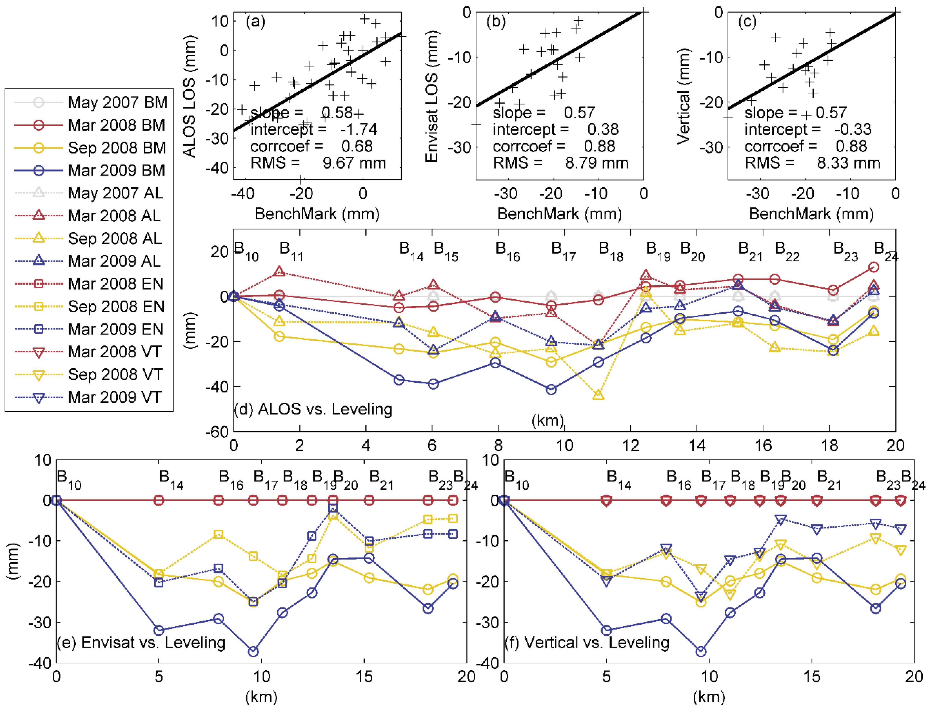
4.2. InSAR and Leveling Comparison

Leveling data are available in May 2007, March 2008, September 2008 and March 2009 from 13 benchmarks along a 20 km section of the Jing-Hu High Speed railway in this area. InSAR results are compared with the leveling survey results. Comparison between InSAR and leveling is not straightforward due to different reference systems. Leveling reference point for Tianjin is the Liqizhuang bedrock point located in Tianjin institution of surveying and mapping. Liqizhuang bedrock point is a deep stratum benchmark, with its base 1088 m underground in Cambrian formations [41]. The InSAR results are referenced to the mean value of phases first. Then, the areas with the greatest uplift signals are chosen as the InSAR reference area. Comparison between leveling and InSAR displacements can be made through a double difference in time and space [42]. The spatial reference for InSAR and leveling comparison is leveling point BM2010, which exhibited the least subsidence among all leveling points. The temporal reference for InSAR and leveling comparison is set at the first leveling campaign in May 2007. Firstly, LOS InSAR displacements are linearly interpolated at the leveling times. Secondly, Interpolated LOS InSAR results are double differenced using the spatial and temporal reference. Finally, LOS Envisat and ALOS results are decomposed into east-west and vertical components by ignoring north-south horizontal movement for a polar orbit SAR satellite [43]. To be consistent with InSAR results, the leveling results are re-referenced to BM2010 at May 2007 as well. It should be noted that first Envisat acquisition is later than first leveling campaign, so InSAR and leveling results are temporally re-referenced to March 2008 when necessary.
The RMS differences are 9.7 mm between ASAR LOS and leveling, 8.8 mm between PALSAR and leveling, and 8.3 mm between vertical component and leveling (Figure 4a–c). Slightly improvement is seen after decomposition of horizontal movement from vertical (Figure 4c,f). The reason lies in the fact that the accuracy of Leveling data, interpolated ALOS and Envisat displacement is limited. On the one hand, the accuracy of interpolated ALOS and Envisat displacement is limited by seasonal movement. For example, ALOS displacement on 1 March 2009 is interpolated from displacements of 22 January and 9 March 2009, while Envisat displacement on 1 March 2009 is interpolated from displacements of 27 February and 3 April 2009. The water level began to drop in late March, so the interpolated Envisat displacement is greater than ALOS in March 2009. It seems that the decomposition of horizontal and vertical movement is not highly effective in the presence of seasonal displacement. On the other hand, the leveling dates available are only accurate to months, and the first day of the month is assumed as the leveling date for a campaign. However, it still can be seen that interpolated ALOS and Envisat displacements generally follow the displacement trend of benchmarks, although with less displacement (Figure 4d,e). It is likely that the vertical displacement is dominant to horizontal displacement along the leveling line, and the projection from vertical to LOS results in displacement reduction for both ascending and descending tracks.

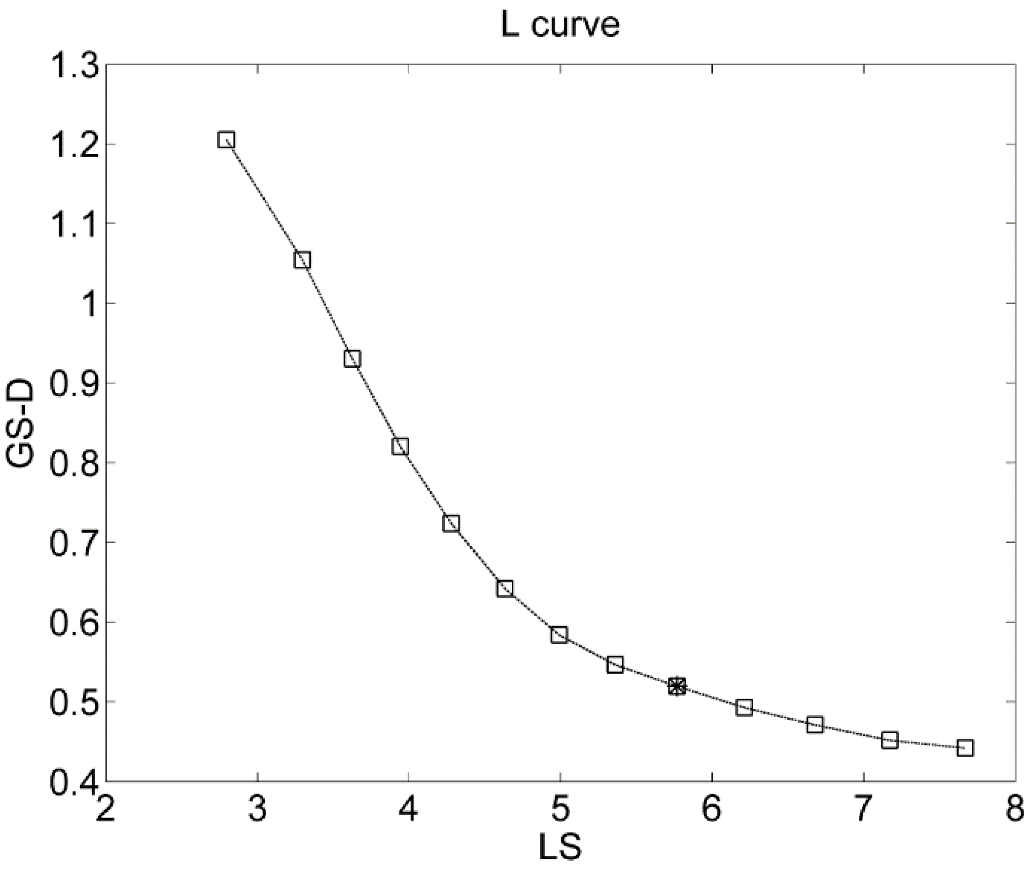
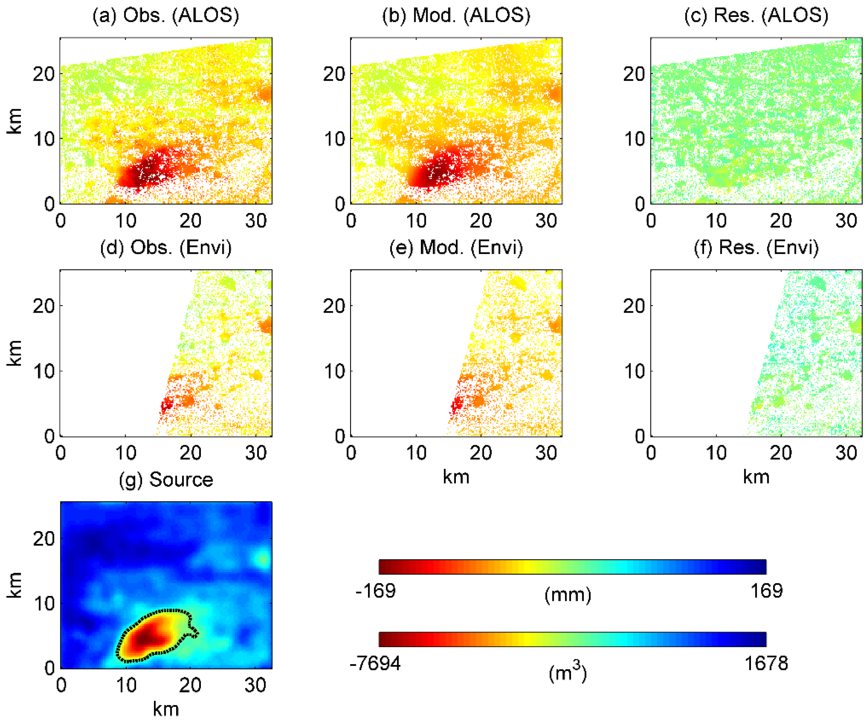
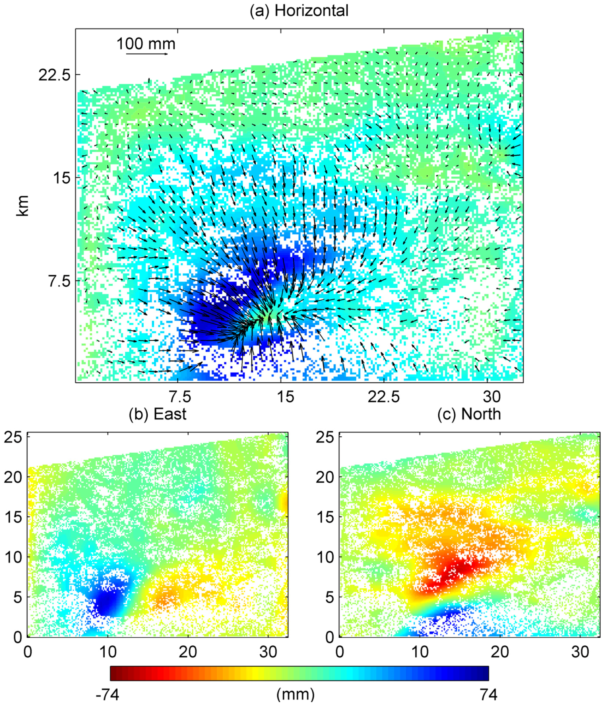
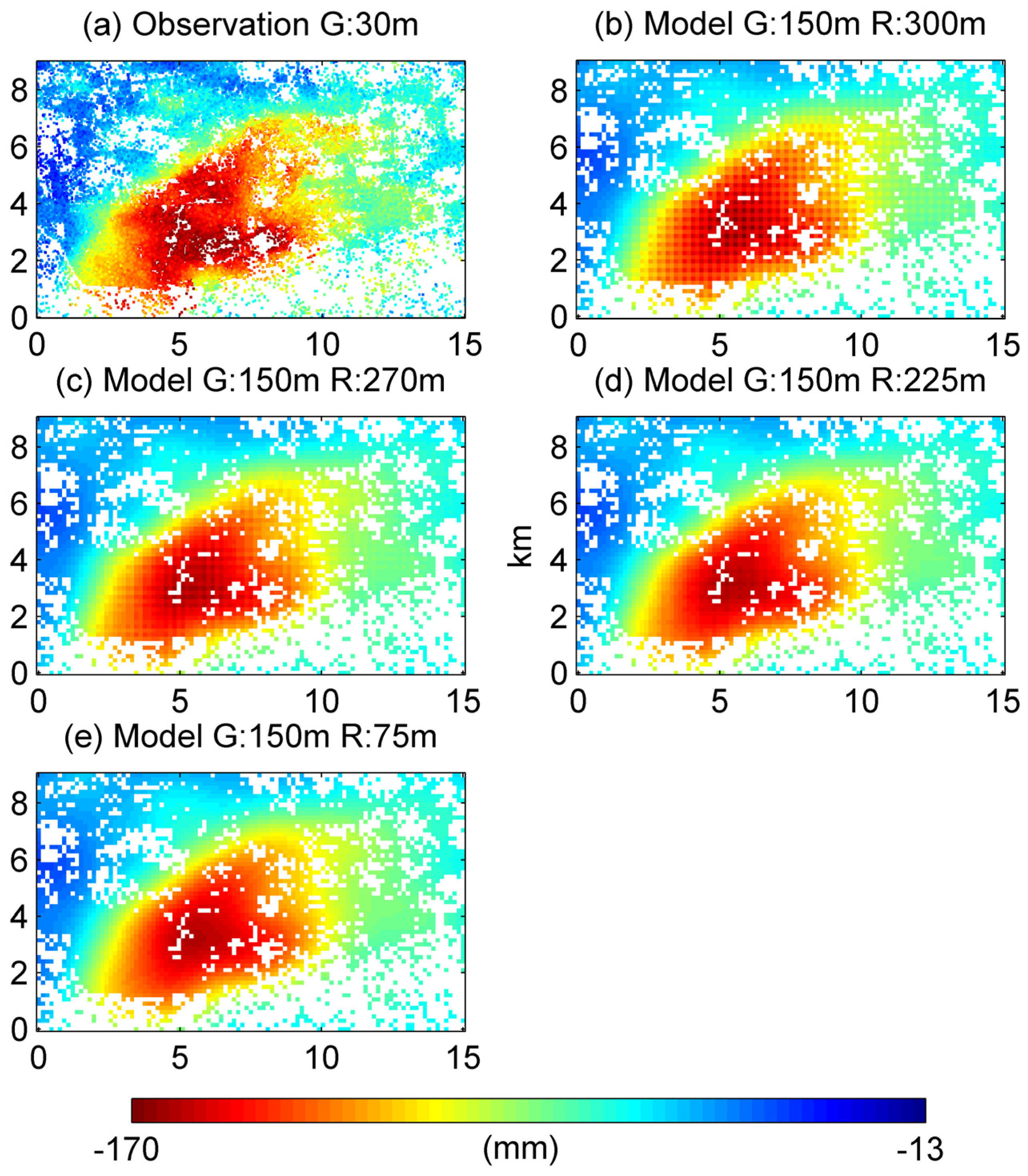
4.3. Model of West Subsidence

The western subsidence is modeled using Mogi source solution in a semi-analytical approach [44,45].
u z ( x , y ) = i ( 1 ν ) Δ V i π g z ( r i , d )
g z ( r , d ) = d ( r 2 + d 2 ) 3 / 2
r i = ( x x i ) 2 + ( y y i ) 2
where u z ( x , y ) is the vertical displacement at ( x , y ) , Δ V i is the volume change at reservoir element i , g z ( r , d ) is the vertical green/influence function, ν . is the Poisson’s ratio, r i is horizontal distance between surface point ( x , y ) and reservoir element ( x i , y i ) , d is reservoir depth. The reservoir is divided into equal squares.
A semi analytical inversion is performed for Mogi source array to determine the best fit distribution of source volume change for LOS annual displacements (annual rates times one year). Modeled surface displacements are the ensemble contributions from each source. Poisson’s ratio of 0.25 is set for this study. Reservoir depth is fixed at about 200 meters as ground water is pumped from a depth of 100–300 m in Tianjin [7]. The linear least-squares inversion procedure has been adopted to estimate the source volume change.
It is well known that InSAR observations may contain global bias due to uncertainties in reference level or other uniform signals (e.g., sediment compaction). Accordingly, a constant offset is allowed in model inversion to accommodate the global bias.
In the process of inversion, regularization on the source strength is often needed to ensure a reliable inversion with a faithful representation of the source. Directly modeled reservoir volume changes (Figure 5a) seem noisier than the regularized source (Figure 5b). This can be caused by displacement uncertainty due to noise and other error sources. Besides, the semi analytical approach allows approximation of reservoir change and efficient computations, but it does not assure the physical process that must involve a continuous contracting/inflating volume. A Laplacian regularization based process was applied to smooth the source (Figure 5b).
( G 1 L F 0 ) ( S O ) = ( D 0 )
where G is the Green’s function, L is the Laplacian smooth operator, F is the smoothing factor (weight), and their product L F is the smoothing matrix used in model inversion. S is the source volume change, O is the offset term for global bias, and D is the observed displacement. In order to balance the roughness of source volume change and model fit to displacement, the L curve method (Figure 6) is adopted to find the best smoothing factor [46].
The modeled source volume change is about −7694 to +1678 m3 for each element (300 m square) per year (Figure 7), equivalent to water volume change of −85,000 to +18,000 m3/km2/year, further equivalent to water storage change of −85 to +18 mm·year−1 in height. Unfortunately, to the best of our knowledge, in situ measurements of fluid volume from production wells is unpublished and is not available for comparison with our modeling results. Ground water storage (GWS) change from GRACE satellite measurement is about −17 to −22 mm·year−1 in North China Plain [47,48,49], equivalent to −17,000 to −22,000 m3/km2/year. The GRACE measurement covers Beijing, Tianjin, Hebei and Shanxi of ~370,000 km2, while our model is in an area of 860 km2 in Tianjin. Simulated recoverable groundwater storage depletion is −30,000 m3/km2/year (equivalent to 30 mm·year−1 in height) from 1970 to 2008 [50], equivalent to −2700 m3 for each element (source) per year. Contour line of −2700 m3 is superimposed on source volume change (Figure 7d). Line −2700 m3 coincides with sharp reduction of both the water extraction volume and subsidence observed. Modeled source volume change show local water storage increase up to 1678 m3. InSAR observations show subsidence of −168.5 to −2.9 mm in model area (Figure 7a). The volume increase seems to contradict with the fact that only subsidence is observed in this area. From the perspective of semi-analytical modeling, any surface deformation is the ensemble contribution of all model sources via their influence functions. Therefore, for a surface point, the superposition of a remote contracting source with large volume decrease, and a nearby inflating source with small volume increase, may still generate a surface subsidence. From the perspective of physical process, aquifer can benefit from precipitation infiltration, irrigation return, or other vertical or horizontal recharge. For instance, rainfall in summer recharge local ground water aquifers in North China Plain by 12–29 mm seen from GRACE and 25 mm seen from ground boreholes [48].
The horizontal displacement can be modeled using horizontal Green’s function and the best-fit source volume change.
g r ( r , d ) = r ( r 2 + d 2 ) 3 / 2
where g r ( r , d ) is the horizontal green/influence function. Modeled horizontal displacements can be substantial, with maximum annual horizontal displacements reach up to 74 mm (Figure 8). Maximum horizontal displacements are located along a semi closed oval around the modeled source center. The modeled maximum horizontal displacement is 36% of the maximum vertical displacement. Theoretical ratio of maximum horizontal to maximum vertical displacement is 38% for a single Mogi source [51]. A field based aquifer test in Nevada shows that the horizontal displacements reach 8 mm and vertical displacements reach 12 mm within the first 22 days of pumping before reaching the steady state pumping [52]. Thus, the horizontal displacement induced by aquifer abstraction can be significant. Horizontal displacements are believed to be a cause of ground fissures [53]. Ground fissures associated with subsidence has caused severe infrastructure damage in Taiyuan Basin of China [54]. Hence, it is worth measuring the horizontal displacements due to ground water depletion, including Tianjin.

5. Discussion

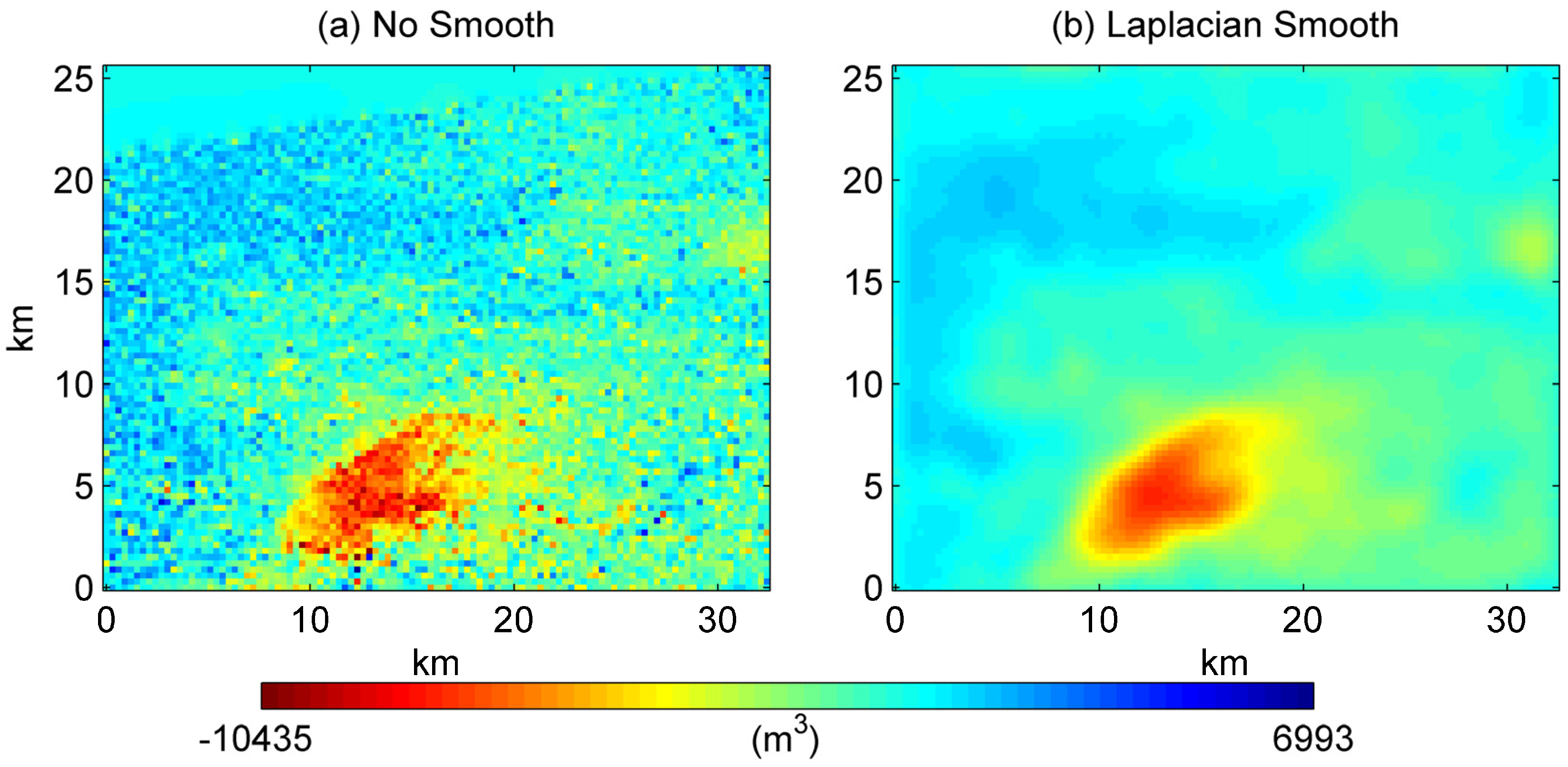
5.1. Impact of Reservoir Grid Size

Grid-like patterns stand out in the modeled displacement (Figure 9b). The hypotheses that these are related with reservoir grid size are examined. The 300 m reservoir is now resampled into 270 m, 225 m, and 75 m grids (Figure 9c–e). At the same time, reservoir volume changes are resampled by size to fit the surface displacement. It can be seen that surface displacements are well represented when finer reservoir grids are adopted without alternating surface grid size. Hence, the grid patterns that obscure the modeled displacement are mainly due to the reservoir grid size in this case.
It should be noted that Mogi-type modeling assumes that source radius α is much smaller than source depth ((α/d)→0). A radius of 1 km is usually assumed for volcano cases [51]. The maximum displacement for a finite sphere is about 1 + (α/d)3 times of that for a point sphere [51]. Accordingly, the grid-like patterns appear when the ratio of cavity radius to depth is significant (Figure 9). Hence, water storage change can be underestimated when reservoir grid size is similar to its depth. However, fine reservoir grid causes quadratic growth of source numbers, greatly increasing computational burden in model inversion.

5.2. Tectonic Division and Its Effect on Subsidence

There are two kinds of explanations when fault act as a subsidence barrier. First, sediment deposits separated by the fault exhibit different compressibility [55]. Second, ground water hydraulic conductivity is low around the fault [56]. In this section, major faults in Tianjin are examined to see if they are related with subsidence observed. The tectonic division could help address the subsidence differences seen in Tianjin.
The east subsidence, outlined by B1 in Figure 10b, is controlled by Tianjinbei fault to the west, and Dasi fault to the east. Most of the east subsidence is located in the area of Shuangyao salient.
Velocity differences (abrupt InSAR mean velocity changes) can be found between the areas to the west and to the east of lines F1, F2, and F3 (The F lines in Figure 10b are drawn by visual inspection) (Figure 10b). Line F1 coincides with a fault to the west of Baitangkou depression [57]. Line F2 matches the central segment of Dasi fault [58]. Dasi fault is also known as Baitangkou fault. Line F3, however, bends away from Dasi fault and is oriented in NE-SW direction. It remains unclear if a fault exists along F3. Further geological investigation is needed to confirm this.
The Tianjinbei fault is striking NNE (strike is a line representing the intersection of a fault with a horizontal plane) and dipping NW (dip is the angle of descent of a fault relative to a horizontal plane). The Tianjinnan fault is also striking NNE while dipping SE. The Tianjinbei fault and the Tianjinnan fault are 6–7 km apart. Tianjinbei fault joins Haihe fault to the north in Tianjin city center [59]. A velocity strip (a long and narrow zone with mean velocities different from neighboring area) matches the location of the Tianjinnan fault (Figure 10). Dislocated stratum appears at about 47 m in depth from TJ08 seismic profile of Tianjinnan fault [59]. Boreholes TS1 and TS4 near profile TJ08 show that a 9.5 m fault throw (the vertical component of the dip separation) appears at 88.3–90.3 m in depth to the west of Tianjinnan fault and at 98.9–99.7 m in depth to the east of Tianjinnan fault [60].
Haihe fault separates Tianjinbei fault into north and south segments. A velocity strip matches the north segment of Tianjinbei fault (Figure 10). In the north segment, dislocated stratum appears at 132 m and 125 m in depth from TJ01 and SY02 seismic profiles of Tianjinbei fault [59]. Weak velocity differences can also be observed along line F4 (Figure 10b), which can be the south segment of Tianjinbei fault.
Cangdong fault is striking NNE and dipping SE. Tianjin segment of Cangdong fault is cut by Baodi fault and haihe fault [62]. Velocity differences are seen along lines F6 and F7 (Figure 10b). Dislocated stratum appears at 152 m in depth from TJ23 seismic profile of Cangdong fault [59].
Haihe fault is striking NW to NWW and dipping SSW [59]. Distinguishable minimum depth of Haihe fault is 60–70 m [59]. It crosses the Tianjin urban area where uniform velocities are observed.
The east subsidence area shows greater subsidence rates than urban areas of Tianjin on both Envisat and ALOS mean velocity maps. This is consistent with the fact that the area of ground water extraction expanded to the suburban area since 1990s and the ground water pumping volume in urban area has declined from more than 100 million in 1981 to less than 10 million cubic meters in 2007 [5].
Within a geological uplift, the east subsidence is likely the result of heavy underground water use. Geological control of the east subsidence is seen along DSF and TJBF. Subsidence is likely to be related with stratum below 125 m seen from TJBF.

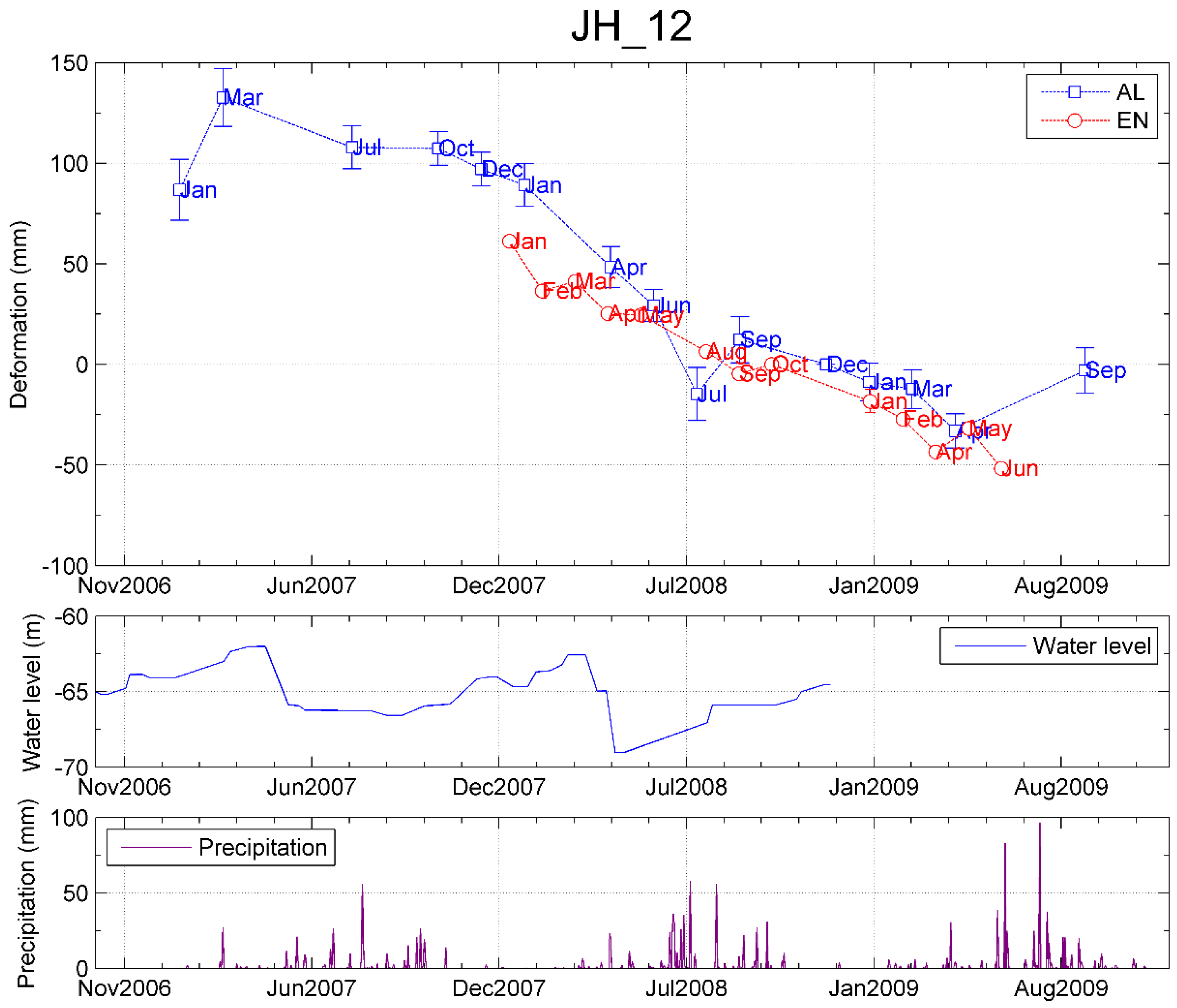
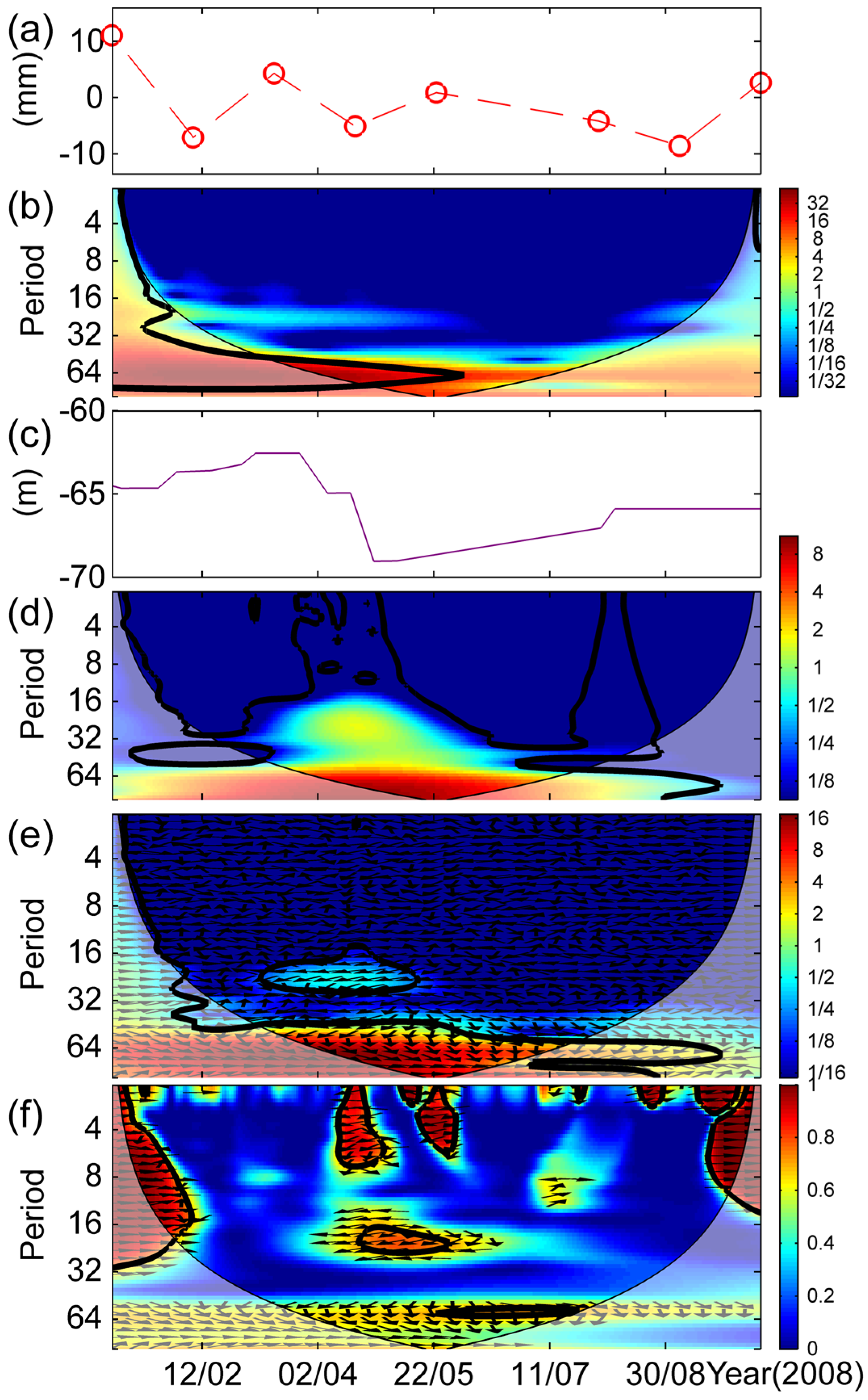
5.3. Water Level and Subsidence

In the east subsidence, the time series displacement of JH-12 Well is plotted against contemporary precipitation and its water level records of Aquifer II (Figure 11). It can be seen that seasonal InSAR displacements near JH-12 generally follows the underground water levels of JH-12. North China Plain is one of the largest agricultural production area in China, accounting for about 50% of wheat and 33% of maize grain production in China [63]. The boot growth stage of winter wheat is April, when water demand by irrigation reaches its peak level. The water table was the lowest from May to June each year. The irrigation return and abundant precipitation in July and August infiltrated and recharged ground water [64]. The water level then rose to the highest level in March or April the following year.
The water level pattern of JH-12 resembles the lateral recharge-runoff-discharge pattern in the piedmont of North China Plain [66]. However, JH-12 is at least 100 km away from the piedmont plain zone besides Yanshan Mountain and Taihang Mountain, and is located in alluvial fan and flood plain [67]. In central North China Plain, water level is normally low in winter and spring with strong evaporation and less precipitation [66], while JH-12 show consistently high water level in winter and spring except a tiny fluctuation of ca. 0.5 m around December (Figure 11). It is likely that JH12 is laterally recharged since Tuanbo Reservoir is nearby (Figure 12b).
Water level of JH-12 declines sharply from −62.57 m to −69.03 m between 23 March and 26 April 2008. Consequent subsidence between 21 April and 22 July in 2008 reaches about 63 mm in ALOS LOS direction. The short term aquifer compaction should be elastic as the water level recovers to a nearly identical level next march. Hence we evaluate the elastic storage coefficient S ke * near JH-12 by relating aquifer compaction and effective stress change. Aquifer compaction and stress change are reflected by ALOS displacement and hydraulic head change respectively [68]. The seasonal LOS deformation, satellite incidence angle, and water level drop, yield an elastic storage coefficient of 0.0125 for JH-12 from ALOS. Although 18 mm LOS subsidence is observed between 23 May and 1 August 2008 from Envisat, no ASAR image can be found in June or July, when subsidence reaches its maximum value seen from ALOS.
In a numerical study of flow system simulation in the North China Plain, storage parameter set for Aquifer III is in the range of 0.0001–0.005 with geometric mean value of 0.0012, and storage parameter set for Aquifers I and II are in the range of 0.04–0.25 with geometric mean of 0.075 [50]. The elastic storage near JH-12 Well triples the maximum storage parameter set for Aquifer III, but is merely one-third of the minimum storage parameter set for Aquifers I and II [50]. Hence Aquifer II and other aquifer layers are likely contribute together to the observed surface subsidence.
Subsidence rates are compared with water level of Aquifer III and Aquifer IV in 2008 [26] (Figure 12). Notably, the water levels are relative because the depth of Aquifer III and Aquifer IV are in the range of 180–400 m for the east subsidence area in their paper. The water level in Aquifer III of the east subsidence area is −70 to −60 m in depth, while it is >−55 m in the urban area of Tianjin in 2008. Higher subsidence rates are associated with lower water level in Aquifer III. Aquifer III is likely to be a subsidence source to the east subsidence due to similarity in map patterns between subsidence and lower water levels. Correlation between the water level of Aquifer IV and subsidence pattern are not seen.
A wavelet analysis on InSAR displacement and water level time series is implemented (Appendix). Displacement periodicities and time shift between water level and displacement time series are analyzed.

6. Conclusions

Subsidence up to 170 mm·year−1 is observed in the Tianjin Municipality from Envisat/ASAR and ALOS/PALSAR images collected between 2007 and 2009. The subsidence rates are similar across the overlap area between Envisat and ALOS results. Subsidence along the JH High Speed Railway has also been verified by four leveling campaigns between 2007 and 2009 with a RMS difference of 8–9 mm between InSAR and leveling.
The west subsidence is modeled using Mogi source array. Best-fit water extraction volume is obtained through model inversion. Estimated water volume change is −85,000 to +18,000 m3/km2/year (equivalent to −85 to +18 mm·year−1 in height). High gradients of subsidence and water storage change are associated with the recoverable water volume change of −30,000 m3/km2/year (equivalent to −30 mm·year−1 in height) from other numerical simulation study.
Geological control of Tianjinnan, Tianjinbei and Dasi faults on the east subsidence can be seen from InSAR displacement rates. The east subsidence can be related with Aquifer II, seen from temporal association of subsidence and water level of JH12. The east subsidence can also be related with Aquifer III, seen from elastic storage coefficient and spatial association of subsidence and water level of Aquifer III.
This study demonstrates the capability of time series InSAR to map subsidence, model ground water volume change, identify geological control factors, and estimate storage coefficients in Tianjin. InSAR can be an effective tool to investigate ground water use conditions in Tianjin and NCP.

Acknowledgments

This work is supported by a NSFC (National Natural Science Foundation of China) Program to Peng Liu (No. 41504003), a NSFC program to Chisheng Wang (No. 41504004), and Shenzhen-Hong Kong Innovation Circle Program (No. SGLH20150206152559032) to Peng Liu and Chisheng Wang. The ENVISAT images were supplied through the ESA-MOST Dragon 2 Cooperation Program (ID: 5343). Qingquan Li is supported by grants from Shenzhen Scientific Research and Development Funding Program (No. ZDSY20121019111146499 and No. JSGG20121026111056204), Shenzhen Dedicated Funding of Strategic Emerging Industry Development Program (No. JCYJ20121019111128765), and Shenzhen Future Industry Development Funding Program (No. 201507211219247860). Zhenhong Li is supported by the UK Natural Environmental Research Council (NERC) through the LICS project (ref. NE/K010794/1), the ESA-MOST DRAGON-3 projects (ref. 10607 and 10665) and Open Fund from the Key Laboratory of Earth Fissures Geological Disaster, Ministry of Land and Resources (Geological Survey of Jiangsu Province). We thank JPL/Caltech for the use of ROI PAC, TU-Delft for DORIS and Andy Hooper for StaMPS in our data processing and analysis. Part of the figures were prepared using the public domain Generic Mapping Tools.

Author Contributions

Peng Liu performed experiments and drafted the manuscripts. Qingquan Li, Zhenhong Li, Trevor Hoey and Guoxiang Liu contributed to InSAR data analysis. Chisheng Wang, Zhongwen Hu, Zhiwei Zhou and Andrew Singleton contributed to model calculations.

Conflicts of Interest

The authors declare no conflict of interest. The founding sponsors had no role in the design of the study; in the collection, analyses, or interpretation of data; in the writing of the manuscript, and in the decision to publish the results.

Abbreviations

The following abbreviations are used in this manuscript:
InSARInterferometric Synthetic Aperture Radar
ASARAdvanced Synthetic Aperture Radar
ALOSAdvanced Land Observing Satellite
PALSARThe Phased Array type L-band Synthetic Aperture Radar
NCPNorth China Plain
ROI_PACRepeat Orbit Interferometry PACkage
DORISThe Delft Object-oriented Radar Interferometric software
StaMPSStanford Method for Persistent Scatterers
SRTMShuttle Radar Topography Mission
PSPersistent Scatter
SDFPSlowly-Decorrelating Filtered Phase
APSAtmospheric Phase Screen
GWSGround Water Storage

Appendix

Wavelet tools are used to analyze the seasonal displacements observed from Envisat and ALOS and the associations between displacements and water level time series at JH-12 Well. The wavelet tools employed in this study are continuous wavelet transform (CWT), cross wavelet transform (XWT), and wavelet coherence (WTC). CWT decomposes one dimensional InSAR time series into two dimensional time frequency space to determine the local periodicities of seasonal variations [69]. The cross wavelet transform (XWT) and wavelet coherence (WTC) tools indicate the common power and relative phase between the two time series [70,71].
Common interval for Envisat displacement and water level time series is between 4 January 2008 and 10 October 2008. Linear component of Envisat displacements is estimated by least square method and subtracted from the time series. The Envisat image number is limited to eight, and down sampling of water level time series at image acquisition time results in very coarse power spectrum. Oppositely, the non-linear component of Envisat displacement is over sampled by linear interpolation at water level time. However, the interpolation also reduces the accuracy of displacements. Envisat time series show a two-month cycle (64-day period) between April and May 2008 from CWT analysis (Figure A1b). No effective cycle can be observed for water level time series (Figure A1d). XWT analysis shows a phase rotation from about 120° out of phase in the one and half month cycle (48-day period) to about 120° in phase in the two month cycle (64-day period) between April and May 2008 (Figure A1e). Abrupt phase changes occur between adjacent 48-day band and 64-day band. This implies strong seasonal variations in a short time. It corresponds to the quick water level drop in April. WTC analysis shows about 90° out of phase in cycles of 4–8 days and 16–32 days (Figure A1f). It means the displacement leads water level by 1–2 days or 4–8 days. Actually, this is due to lower temporal resolution of Envisat images compared with water level time series. The lowest water level is between the 4th and 5th Envisat image acquisition time, so it looks as if displacement from 4th to 5th image happens before the water level rise. In fact, the 4th image corresponds to a water drop stage while the 5th image corresponds to a water rise stage.
Figure A1. (a) Detrend of Envisat time series at JH-12 Well; (b) continuous wavelet power of the Envisat time series; (c) water level of JH-12 Well; (d) continuous wavelet power of water level time series; (e) cross wavelet transform of Envisat and water level time series at JH-12 Well; and (f) wavelet coherence of Envisat and water level time series for JH-12. Images (gl) are the same for ALOS and water level time series at JH-12 Well. The thick contour is the 95% confidence level. The cone of influence (COI) is shown in light shadow.
Remotesensing 08 00266 g013aRemotesensing 08 00266 g013b
Common interval for ALOS and water level time series is from 17 January 2007 to 7 December 2008. CWT analysis of ALOS time series shows a four-month cycle (128 days) between the 8th (6 June 2008) and the 10th (6 September 2008) ALOS image. CWT analysis for water level time series also shows a 128-day cycle, though at a lower confidence level. XWT analysis show 90° in phase in the 80-day band and 90° out of phase in the 128-day band, from the 6th (20 January 2008) to the 9th (22 July 2008) ALOS image. This means strong seasonality occurs between the two images. WTC analysis shows about 90° in phase in cycles of 4–8 days near the 7th ALOS image (21 April 2008). This means water level leads displacement by 1–2 days, which is beyond the 46-day repetition frequency of ALOS acquisition. WTC analysis also shows 90° in phase in cycles of 64 days between 7th (21 April 2008) and 10th (6 September 2008) ALOS image, although with lower confidence level. It means water level leads displacement by 16 days. The displacement began to stabilize at the 10th (6 September 2008) ALOS image, while the water level’s recent rise stops at 8 August 2008, which is about 29 days ahead of the 10th ALOS image. The phase shift of 16 days between water level and displacement time series can be explained by the delay of 29 days. Moreover, it also implies the deformation may have already stabilized before 6 September 2008, because the phase (time) shift from continuous wavelet analysis is more robust than direct comparison of isolated time series points.
Wavelet tools are able to find the periodicities of InSAR time series and relative phase (time) shift between InSAR and water level time series. However, the wavelet power spectrum can be misleading if the temporal resolution of time series is low. Meanwhile, the phase (time) shift from continuous wavelet analysis enhances the robustness of time delay analysis between time series.

References

  1. Chaussard, E.; Wdowinski, S.; Cabral-Cano, E.; Amelung, F. Land subsidence in central Mexico detected by ALOS InSAR time-series. Remote Sens. Environ. 2014, 140, 94–106. [Google Scholar] [CrossRef]
  2. Osmanoglu, B.; Dixon, T.H.; Wdowinski, S.; Cabral-Cano, E.; Jiang, Y. Mexico city subsidence observed with persistent scatterer InSAR. Int. J. Appl. Earth Observ. Geoinform. 2011, 13, 1–12. [Google Scholar] [CrossRef]
  3. Hu, B.; Wang, H.-S.; Sun, Y.-L.; Hou, J.-G.; Liang, J. Long-term land subsidence monitoring of Beijing (China) using the small baseline subset (SBAS) technique. Remote Sens. 2014, 6, 3648–3661. [Google Scholar] [CrossRef]
  4. National Bureau of Statistics of the People’s Republic of China. Population of Tianjin in 2010 from Sixth Nationwide Population Census. Available online: http://www.Stats.Gov.Cn/tjsj/tjgb/rkpcgb/dfrkpcgb/201202/t20120228_30405.Html (accessed on 11 Novermber 2015). (In Chinese)
  5. Yi, L.; Zhang, F.; Xu, H.; Chen, S.; Wang, W.; Yu, Q. Land subsidence in Tianjin, China. Environ. Earth Sci. 2010, 62, 1151–1161. [Google Scholar]
  6. Hu, R.L.; Yue, Z.Q.; Wang, L.C.; Wang, S.J. Review on current status and challenging issues of land subsidence in China. Eng. Geol. 2004, 76, 65–77. [Google Scholar] [CrossRef]
  7. Hu, R.L.; Wang, S.J.; Lee, C.F.; Li, M.L. Characteristics and trends of land subsidence in Tanggu, Tianjin, China. Bull. Eng. Geol. Environ. 2002, 61, 213–225. [Google Scholar]
  8. Luo, Q.; Perissin, D.; Zhang, Y.; Jia, Y. L- and X-band multi-temporal InSAR analysis of Tianjin subsidence. Remote Sens. 2014, 6, 7933–7951. [Google Scholar] [CrossRef]
  9. Zhang, K.; Ge, L.; Li, X.; Ng, A.-M. Monitoring ground surface deformation over the North China Plain using coherent ALOS PALSAR differential interferograms. J. Geod. 2013, 87, 253–265. [Google Scholar] [CrossRef]
  10. Liu, G.; Jia, H.; Nie, Y.; Li, T.; Zhang, R.; Yu, B.; Li, Z. Detecting subsidence in coastal areas by ultrashort-baseline TCPInSAR on the time series of high-resolution TerraSAR-X images. IEEE Trans. Geosci. Remote Sens. 2014, 52, 1911–1923. [Google Scholar]
  11. Chen, J.; Wu, J.; Zhang, L.; Zou, J.; Liu, G.; Zhang, R.; Yu, B. Deformation trend extraction based on multi-temporal InSAR in Shanghai. Remote Sens. 2013, 5, 1774–1786. [Google Scholar] [CrossRef]
  12. Erban, L.E.; Gorelick, S.M.; Zebker, H.A. Groundwater extraction, land subsidence, and sea-level rise in the Mekong Delta, Vietnam. Environ. Res. Lett. 2014, 9. [Google Scholar] [CrossRef]
  13. Higgins, S.A.; Overeem, I.; Steckler, M.S.; Syvitski, J.P.M.; Seeber, L.; Akhter, S.H. InSAR measurements of compaction and subsidence in the Ganges-Brahmaputra Delta, Bangladesh. J. Geophys. Res. Earth Surf. 2014, 119, 1768–1781. [Google Scholar] [CrossRef]
  14. Dehghani, M.; Valadan Zoej, M.J.; Hooper, A.; Hanssen, R.F.; Entezam, I.; Saatchi, S. Hybrid conventional and persistent scatterer SAR interferometry for land subsidence monitoring in the Tehran Basin, Iran. ISPRS J. Photogramm. Remote Sens. 2013, 79, 157–170. [Google Scholar] [CrossRef]
  15. Motagh, M.; Walter, T.R.; Sharifi, M.A.; Fielding, E.; Schenk, A.; Anderssohn, J.; Zschau, J. Land subsidence in Iran caused by widespread water reservoir overexploitation. Geophys. Res. Lett. 2008, 35, 428–451. [Google Scholar] [CrossRef]
  16. Anderssohn, J.; Wetzel, H.-U.; Walter, T.R.; Motagh, M.; Djamour, Y.; Kaufmann, H. Land subsidence pattern controlled by old alpine basement faults in the Kashmar Valley, Northeast Iran: Results from InSAR and levelling. Geophys. J. Int. 2008, 174, 287–294. [Google Scholar] [CrossRef]
  17. Motagh, M.; Djamour, Y.; Walter, T.R.; Wetzel, H.-U.; Zschau, J.; Arabi, S. Land subsidence in Mashhad Valley, Northeast Iran: Results from InSAR, levelling and GPS. Geophys. J. Int. 2007, 168, 518–526. [Google Scholar] [CrossRef]
  18. Keiding, M.; Árnadóttir, T.; Jónsson, S.; Decriem, J.; Hooper, A. Plate boundary deformation and man-made subsidence around geothermal fields on the Reykjanes Peninsula, Iceland. J. Volcanol. Geotherm. Res. 2010, 194, 139–149. [Google Scholar] [CrossRef]
  19. Han, Z.; Wu, L.; Ran, Y.; Ye, Y. The concealed active tectonics and their characteristics as revealed by drainage density in the North China Plain (NCP). J. Asian Earth Sci. 2003, 21, 989–998. [Google Scholar] [CrossRef]
  20. Yang, F.; Pang, Z.; Lin, L.; Jia, Z.; Zhang, F.; Duan, Z.; Zong, Z. Hydrogeochemical and isotopic evidence for trans-formational flow in a sedimentary basin: Implications for CO2 storage. Appl. Geochem. 2013, 30, 4–15. [Google Scholar] [CrossRef]
  21. Yao, Z.; Guo, Z.; Xiao, G.; Wang, Q.; Shi, X.; Wang, X. Sedimentary history of the western bohai coastal plain since the late pliocene: Implications on tectonic, climatic and sea-level changes. J. Asian Earth Sci. 2012, 54–55, 192–202. [Google Scholar] [CrossRef]
  22. Minissale, A.; Borrini, D.; Montegrossi, G.; Orlando, A.; Tassi, F.; Vaselli, O.; Huertas, A.D.; Yang, J.; Cheng, W.; Tedesco, D.; et al. The Tianjin geothermal field (North-Eastern China): Water chemistry and possible reservoir permeability reduction phenomena. Geothermics 2008, 37, 400–428. [Google Scholar] [CrossRef]
  23. Xu, H. Stratigraphy and sedimentary features of paleogene sediments of Bohai bay basin. Mar. Geol. Res. 1981, 1, 11–27. (In Chinese) [Google Scholar]
  24. Jia, S.; Zhang, C.; Zhao, J.; Fang, S.; Liu, Z.; Zhao, J. Crustal structure of the rift-depression basin and Yanshan uplift in the northeast part of North China. Chin. J. Geophys. 2009, 52, 51–63. [Google Scholar] [CrossRef]
  25. Zhang, Y.; Meng, P.; Teng, J. Crustal structure and its tectonic responses during mesozoic and cenozoic in Beijing-Tianjin-Tangshan and its adjacent region. Chin. J. Geophys. 2008, 51, 784–795. [Google Scholar] [CrossRef]
  26. Cui, Y.; Su, C.; Shao, J.; Wang, Y.; Cao, X. Development and application of a regional land subsidence model for the plain of Tianjin. J. Earth Sci. 2014, 25, 550–562. [Google Scholar] [CrossRef]
  27. Yang, Y.; Li, X.; Wang, L.; Li, C.; Liu, Z. Characteristics of the groundwater level regime and effect factors in the plain region of Tianjin city. Geol. Surv. Res. 2011, 34, 313–320. (In Chinese) [Google Scholar]
  28. Rosen, P.A.; Hensley, S.; Joughin, I.R.; Li, F.K.; Madsen, S.N.; Rodriguez, E.; Goldstein, R.M. Synthetic aperture radar interferometry. Proc. IEEE 2000, 88, 333–382. [Google Scholar] [CrossRef]
  29. Massonnet, D.; Feigl, K.L. Radar interferometry and its application to changes in the earth’s surface. Rev. Geophys. 1998, 36, 441–500. [Google Scholar] [CrossRef]
  30. Kampes, B.M. Radar Interferometry, Persistent Scatterer Technique; Springer: Berlin, Germany, 2006; Volume 12. [Google Scholar]
  31. Farr, T.G. The shuttle radar topography mission. Rev. Geophys. 2007, 45, 37–55. [Google Scholar] [CrossRef]
  32. Hooper, A.; Segall, P.; Zebker, H.A. Persistent scatterer interferometric synthetic aperture radar for crustal deformation analysis. J. Geophys. Res. 2007, 112, 1–21. [Google Scholar] [CrossRef]
  33. Hooper, A.; Zebker, H.; Segall, P.; Kampes, B. A new method for measuring deformation on volcanoes and other natural terrains using InSAR persistent scatterers. Geophys. Res. Lett. 2004, 31, 275–295. [Google Scholar] [CrossRef]
  34. Ferretti, A.; Prati, C.; Rocca, F. Permanent scatterers in SAR interferometry. IEEE Trans. Geosci. Remote Sens. 2001, 39, 8–20. [Google Scholar] [CrossRef]
  35. Colesanti, C.; Wasowski, J. Investigating landslides with space-borne synthetic aperture radar (SAR) interferometry. Eng. Geol. 2006, 88, 173–199. [Google Scholar] [CrossRef]
  36. Liu, P.; Li, Z.; Hoey, T.; Kincal, C.; Zhang, J.; Zeng, Q.; Muller, J.-P. Using advanced InSAR time series techniques to monitor landslide movements in badong of the three gorges region, China. Int. J. Appl. Earth Observ. Geoinform. 2013, 21, 253–264. [Google Scholar] [CrossRef]
  37. Chen, C.W.; Zebker, H.A. Two-dimensional phase unwrapping with use of statistical models for cost functions in nonlinear optimization. J. Opt. Soc. Am. A 2001, 18, 338–351. [Google Scholar] [CrossRef]
  38. Shirzaei, M.; Bürgmann, R. Topography correlated atmospheric delay correction in radar interferometry using wavelet transforms. Geophys. Res. Lett. 2012, 39. [Google Scholar] [CrossRef]
  39. Jolivet, R.; Grandin, R.; Lasserre, C.; Doin, M.P.; Peltzer, G. Systematic InSAR tropospheric phase delay corrections from global meteorological reanalysis data. Geophys. Res. Lett. 2011, 38. [Google Scholar] [CrossRef] [Green Version]
  40. Li, Z.; Fielding, E.J.; Cross, P.; Muller, J.-P. Interferometric synthetic aperture radar atmospheric correction: GPS topography-dependent turbulence model. J. Geophys. Res. 2006, 111, 1059–1075. [Google Scholar] [CrossRef]
  41. Chen, F.; Ji, J.; Han, Y.; Chen, J. Research on vertical stability of Liqizhuang bedrock point. J. Geod. Geodyn. 2013, 33, 49–52. (In Chinese) [Google Scholar]
  42. Leighton, J.M.; Sowter, A.; Tragheim, D.; Bingley, R.M.; Teferle, F.N. Land motion in the urban area of nottingham observed by ENVISAT-1. Int. J. Remote Sens. 2013, 34, 982–1003. [Google Scholar] [CrossRef]
  43. Miller, M.M.; Shirzaei, M. Spatiotemporal characterization of land subsidence and uplift in phoenix using insar time series and wavelet transforms. J. Geophys. Res. Solid Earth 2015, 120, 5822–5842. [Google Scholar] [CrossRef]
  44. Fokker, P.; Orlic, B. Semi-analytic modelling of subsidence. Math. Geol. 2006, 38, 565–589. [Google Scholar] [CrossRef]
  45. McTigue, D.F. Elastic stress and deformation near a finite spherical magma body: Resolution of the point source paradox. J. Geophys. Res. 1987, 92, 12931–12940. [Google Scholar] [CrossRef]
  46. Hansen, P.C. Analysis of discrete ill-posed problems by means of the L-curve. SIAM Rev. 1992, 34, 561–580. [Google Scholar] [CrossRef]
  47. Huang, Z.; Pan, Y.; Gong, H.; Yeh, P.J.F.; Li, X.; Zhou, D.; Zhao, W. Subregional-scale groundwater depletion detected by grace for both shallow and deep aquifers in North China Plain. Geophys. Res. Lett. 2015, 42, 1791–1799. [Google Scholar] [CrossRef]
  48. Shen, H.; Leblanc, M.; Tweed, S.; Liu, W. Groundwater depletion in the Hai River Basin, China, from in situ and grace observations. Hydrol. Sci. J. 2014, 60, 671–687. [Google Scholar] [CrossRef]
  49. Feng, W.; Zhong, M.; Lemoine, J.-M.; Biancale, R.; Hsu, H.-T.; Xia, J. Evaluation of groundwater depletion in north China using the Gravity Recovery and Climate Experiment (GRACE) data and ground-based measurements. Water Resour. Res. 2013, 49, 2110–2118. [Google Scholar] [CrossRef]
  50. Cao, G.; Zheng, C.; Scanlon, B.R.; Liu, J.; Li, W. Use of flow modeling to assess sustainability of groundwater resources in the North China Plain. Water Resour. Res. 2013, 49, 159–175. [Google Scholar] [CrossRef]
  51. Lisowski, M. Analytical volcano deformation source models. In Volcano Deformation; Springer: Berlin, Germany, 2006; pp. 279–304. [Google Scholar]
  52. Burbey, T.J.; Warner, S.M.; Blewitt, G.; Bell, J.W.; Hill, E. Three-dimensional deformation and strain induced by municipal pumping, part 1: Analysis of field data. J. Hydrol. 2006, 319, 123–142. [Google Scholar] [CrossRef]
  53. Yang, C.-S.; Zhang, Q.; Zhao, C.-Y.; Wang, Q.-L.; Ji, L.-Y. Monitoring land subsidence and fault deformation using the small baseline subset insar technique: A case study in the Datong Basin, China. J. Geodyn. 2014, 75, 34–40. [Google Scholar] [CrossRef]
  54. Zhu, W.; Zhang, Q.; Ding, X.; Zhao, C.; Yang, C.; Qu, W. Recent ground deformation of Taiyuan basin (China) investigated with C-, L-, and X-bands SAR images. J. Geodyn. 2013, 70, 28–35. [Google Scholar] [CrossRef]
  55. Amelung, F.; Galloway, D.L.; Bell, J.W.; Zebker, H.A.; Laczniak, R.J. Sensing the ups and downs of Las Vegas: InSAR reveals structural control of land subsidence and aquifer-system deformation. Geology 1999, 27, 483–486. [Google Scholar] [CrossRef]
  56. Chaussard, E.; Bürgmann, R.; Shirzaei, M.; Fielding, E.J.; Baker, B. Predictability of hydraulic head changes and characterization of aquifer-system and fault properties from insar-derived ground deformation. J. Geophys. Res. Solid Earth 2014, 119. [Google Scholar] [CrossRef]
  57. Jiang, G. The Research on the Main Factors of Controlling the Development of Ordovician Geothermal Reservoirs in Tianjin; China University of Geoscience: Beijing, China, 2014. (In Chinese) [Google Scholar]
  58. Lin, L. Sustainable Development and Utilization of Thermal Groundwater Resources in the Geothermal Reservoir of the Wumishan Group in Tianjin; China University of Geosciences: Beijing, China, 2006. (In Chinese) [Google Scholar]
  59. Chen, Y. Tectonic Activity Features and Segmentation of Seismic risk of the Buried Haihe Fault in Tianjin; China Earthquake Administration: Beijing, China, 2007. (In Chinese)
  60. Shao, Y.; Li, Z.; Chen, Y.; Ren, F.; Yao, Z. A study on the quaternary activity of the Tianjin fault. Earthq. Res. China 2010, 24, 353–362. [Google Scholar]
  61. Liu, J. The Geochemical Character of Geothermal Liquid in Tianjin Area; China University of Geoscience: Beijing, China, 2014. (In Chinese) [Google Scholar]
  62. Zhao, S.; Gao, B.; Li, X.; Li, H.; Hu, Y. Character and water temperature conductivity of the Cangdong fault Tianjin segment. Geol. Surv. Res. 2007, 30, 121–127. [Google Scholar]
  63. Wang, J.; Wang, E.; Yang, X.; Zhang, F.; Yin, H. Increased yield potential of wheat-maize cropping system in the North China Plain by climate change adaptation. Clim. Chang. 2012, 113, 825–840. [Google Scholar] [CrossRef]
  64. Lu, X.; Jin, M.; van Genuchten, M.T.; Wang, B. Groundwater recharge at five representative sites in the Hebei plain, China. Groundwater 2011, 49, 286–294. [Google Scholar] [CrossRef] [PubMed]
  65. China Meteorological Administration. Available online: http://data.Cma.Gov.Cn/ (accessed on 20 September 2015). (In Chinese)
  66. Wang, S.; Song, X.; Wang, Q.; Xiao, G.; Liu, C.; Liu, J. Shallow groundwater dynamics in North China Plain. J. Geogr. Sci. 2009, 19, 175–188. [Google Scholar] [CrossRef]
  67. Chen, W.; Qinghai, X.; Xiuqing, Z.; Yonghong, M. Palaeochannels on the North China Plain: Types and distributions. Geomorphology 1996, 18, 5–14. [Google Scholar] [CrossRef]
  68. Hoffmann, J.; Zebker, H.A.; Galloway, D.L.; Amelung, F. Seasonal subsidence and rebound in Las Vegas valley, Nevada, observed by synthetic aperture radar interferometry. Water Resour. Res. 2001, 37, 1551–1566. [Google Scholar] [CrossRef]
  69. Torrence, C.; Compo, G.P. A practical guide to wavelet analysis. Bull. Am. Meteorol. Soc. 1998, 79, 61–78. [Google Scholar] [CrossRef]
  70. Grinsted, A.; Moore, J.C.; Jevrejeva, S. Application of the cross wavelet transform and wavelet coherence to geophysical time series. Nonlinear Process. Geophys. 2004, 11, 561–566. [Google Scholar] [CrossRef]
  71. Tomás, R.; Li, Z.; Lopez-Sanchez, J.M.; Liu, P.; Singleton, A. Using wavelet tools to analyse seasonal variations from InSAR time-series data: A case study of the Huangtupo landslide. Landslides 2015. [Google Scholar] [CrossRef]
Figure 1. (a) The tectonic framework of the Northern China Plain. Boundary of North China Plain is in thick red line. Piedmont plain, alluvial fan and flood plain, and coastal plain in North China Plain are bounded by thick yellow and blue lines. Major faults and subsidiary faults in North China Plain are shown in thin black and red solid lines, respectively [19]. Palaeogene lacuna (missing line of Paleogene system) is in thin dotted line, while further details of the fault system in Tianjin are shown by thin yellow solid lines [20]. Locations of major cities in this area are shown. Envisat ASAR frame, ALOS PALSAR frame, and political boundary of Tianjin are outlined with dashed lines; (b) Annual groundwater pumping volume and rainfall in Tianjin City from 1980 to 2007 (after [5]); (c) Stratigraphy in Bohai Bay Basin (after [21,22,23]). The upper Tertiary formations can be divided into Neogene Minghuazhen (Nm) and Guantao (Ng) groups. The lower Tertiary formations can be divided into Eogene Dongying (Ed), Shahejie (Es), and Kongdian (Ek) formations.
Remotesensing 08 00266 g001
Figure 2. LOS (line of sight) rates from ALOS (17 January 2007 to 9 September 2009) and Envisat (4 January 2008 to 12 June 2009) satellites. Negative values mean moving away from the satellite (e.g., subsidence). The straight line “TJLF (Tianjin Langfang)” is located between Tianjin City and Langfang City. The poly line “HSR (High Speed Railway)” is the path of Jing-Hu high speed railway. The displacement rates along the two swathes are shown in Figure 3. BM2010 and BM2011, along with other benchmarks, are shown in white dots. Leveling results for all benchmarks are compared with InSAR displacements in Figure 4. Reference points for InSAR and leveling are shown in black triangle and dot respectively. Model area is outlined by rectangle. Counties and districts in Tianjin are outlined by thin dashed line. Geothermal fields with gradient above 3.5 (°C/100 m) are outlined by thick dashed line.
Remotesensing 08 00266 g002
Figure 3. (a) LOS rates against longitude in TJLF swath with buffer distance of 500 meters to both sides of the line; and (b) LOS rates against latitude in a swath along the Jing-Hu High Speed Railway with buffer distance of 500 meters to the railway at both sides.
Remotesensing 08 00266 g003
Figure 4. (a) Correlation between ALOS LOS displacements and four leveling campaigns; (b) correlation between Envisat LOS displacements and three leveling campaigns; (c) correlation between decomposed vertical displacements and three leveling campaigns; (d) interpolated ALOS displacements and leveling displacement; (e) interpolated Envisat displacements and leveling displacement; and (f) decomposed vertical displacement and leveling displacement.
Remotesensing 08 00266 g004
Figure 5. Mogi reservoir model: (a) no smooth applied; and (b) Laplacian smooth.
Remotesensing 08 00266 g005
Figure 6. L curve to determine source smoothness. The horizontal axis denotes the modeled source smoothness l o g ( L S 2 ) , where L and S are defined in Equation (4). The vertical axis denotes source fit to InSAR observations l o g ( G S D 2 ) , where G and D are defined in Equation (4). The curve is formed by 13 different Laplacian regularized sources S. Each S corresponds to the best-fit result of each inversion. Smoothing strength for the source is controlled by LF in model inversion. There are 13 smoothing factors F range between 10−4 to 10−1 with exponential step of 0.25. Note that horizontal axis L S is calculated without multiplying smoothing factor F. The square centered with an asterisk represents that a value of 10−3 is employed as the smoothing factor for final result.
Remotesensing 08 00266 g006
Figure 7. (a) ALOS LOS annual displacements (annual rates times one year); (b) modeled ALOS LOS annual displacement; (c) residuals between observed and modeled displacements for ALOS; (d) Envisat LOS annual displacements; (e) modeled Envisat LOS annual displacement; (f) residuals between observed and modeled displacements for Envisat; and (g) modeled Source array volume changes from ALOS displacement. Dashed line is a contour of −2700 m3.
Remotesensing 08 00266 g007
Figure 8. Modeled annual: (a) horizontal displacements; (b) horizontal displacements in E-W direction; and (c) horizontal displacements in N-S direction.
Remotesensing 08 00266 g008
Figure 9. Observed LOS surface displacement (a) and Modeled LOS displacements with reservoir grid size of: (b) 300 m; (c) 270 m; (d) 225 m; and (e) 75 m.
Remotesensing 08 00266 g009
Figure 10. Faults and LOS subsidence rates in Tianjin: (a) Tectonic system of the area includes Dacheng Salient (DCS), Shuangyao Salient (SYS), Panzhuang Salient (PZS), Xiaohanzhuang Salient (XHZS), Litan Depression (LTD), Banqiao Depression (BQD), and Baitangkou Depression (BTKD) [57,58,59,61,62]. Major faults include the Tianjinnan Fault (TJNF), Tianjinbei Fault (TJBF), Dasi Fault (DSF), Haihe Fault (HHF) and Cangdong Fault (CDF); (b) TJ01 and SY02 are seismic profile of TJBF. TJ08 is seismic profile of TJNF, and TS1 and TS4 are boreholes near TJ08. TJ23 is seismic profile of CDF [59].
Remotesensing 08 00266 g010
Figure 11. Envisat and ALOS LOS displacement at JH-12 Well (the triangle in Figure 12b) in east subsidence area. Precipitation data are available from China Meteorological Administration, specifically meteorology station No. 54527 in Tianjin [65]. Water level of JH-12 Well in Aquifer II is available to the end of 2008 [27].
Remotesensing 08 00266 g011
Figure 12. Water levels in 2008 superimposed on LOS subsidence rates from Envisat (4 January 2008 to 12 June 2009): (a) Aquifer III; and (b) Aquifer IV. Location of JH-12 Well is marked in triangle. Tuanbo Reservoir is labeled.
Remotesensing 08 00266 g012
Table 1. Bottom depth of aquifers in Tianjin. Baodi fault and Plain of Tianjin are depicted in Figure 1a. Tanggu district is shown in Figure 2.
LocationTanggu District of TianjinPlain to the South of Baodi FaultPlain of Tianjin
Literature[6] (unit: m)[27] (unit: m)[26] (unit: m)
Aquifer I60–70<7040–123
Aquifer II170–190160–220191–202
Aquifer III270–310260–340309–326
Aquifer IV370–400360–430390–405
Aquifer V~550500–550505–544
Aquifer VIN/AN/A608–613
Table 2. Envisat/ASAR archive with acquisition time and length of perpendicular baseline relative to the reference image on 10 October 2008.
SAR ImageAcquisition TimeBaseline Perpendicular
14 January 2008−401 m
28 February 2008289 m
314 March 2008−75 m
418 April 2008270 m
523 May 200832 m
61 August 2008129 m
75 September 2008312 m
810 October 20080 m
923 January 2009164 m
1027 February 2009235 m
113 April 2009624 m
128 May 2009−48 m
1312 June 2009308 m
Table 3. ALOS/PALSAR archive with acquisition time and length of perpendicular baseline relative to the reference image on 7 December 2008.
SAR ImageAcquisition TimeBaseline Perpendicular
117 January 2007295 m
24 March 20071963 m
320 July 20072700 m
420 October 20073154 m
55 December 20073288 m
620 January 20083764 m
721 April 20084866 m
86 June 20084829 m
922 July 20081624 m
106 September 2008−746 m
117 December 20080 m
1222 January 2009484 m
139 March 2009938 m
1424 April 20091490 m
159 September 20091756 m

