Comparison of Small Baseline Interferometric SAR Processors for Estimating Ground Deformation

Abstract

The small Baseline Synthetic Aperture Radar (SAR) Interferometry (SBI) technique has been widely and successfully applied in various ground deformation monitoring applications. Over the last decade, a variety of SBI algorithms have been developed based on the same fundamental concepts. Recently developed SBI toolboxes provide an open environment for researchers to apply different SBI methods for various purposes. However, there has been no thorough discussion that compares the particular characteristics of different SBI methods and their corresponding performance in ground deformation reconstruction. Thus, two SBI toolboxes that implement a total of four SBI algorithms were selected for comparison. This study discusses and summarizes the main differences, pros and cons of these four SBI implementations, which could help users to choose a suitable SBI method for their specific application. The study focuses on exploring the suitability of each SBI module under various data set conditions, including small/large number of interferograms, the presence or absence of larger time gaps, urban/vegetation ground coverage, and temporally regular/irregular ground displacement with multiple spatial scales. Within this paper we discuss the corresponding theoretical background of each SBI method. We present a performance analysis of these SBI modules based on two real data sets characterized by different environmental and surface deformation conditions. The study shows that all four SBI processors are capable of generating similar ground deformation results when the data set has sufficient temporal sampling and a stable ground backscatter mechanism like urban area. Strengths and limitations of different SBI processors were analyzed based on data set configuration and environmental conditions and are summarized in this paper to guide future users of SBI techniques.

1. Introduction and Motivation

Time-series (TS) Synthetic Aperture Radar Interferometry (InSAR) analysis is a type of advanced technique developed to overcome limitations of the classical differential InSAR (DInSAR) method, e.g., temporal and geometrical decorrelation, and also to compensate error contributions from atmospheric distortions, inaccurate terrain-models and uncertain satellite orbits. With extensive series of SAR imagery, TS InSAR analyzes the spatio-temporal properties of the interferometric phase and has been widely applied to reconstruct the ground deformation history in various applications. Depending on the relying ground scatterer types, TS InSAR approaches can be categorized into two broad families: techniques that focus on Persistent Scatterers (PS), namely, Persistent Scatterer interferometry (PSI) approaches (e.g., [1,2,3,4,5]); and methods relying on Distributed Scatterers (DS) that commonly exploit small baseline interferograms (SBI) (e.g., [6,7,8,9,10,11]). The characteristics of PS and DS targets are vastly different (e.g., scatterer size, relative geometry between scatterer and satellite, material composition of scatterers [12,13,14]). Thus, they behave differently in SAR image stacks and require different algorithms to reconstruct their deformation history [15]. The PS targets contain a stable dominant scatterer within a SAR resolution cell, resulting in consistent scattering properties [2]. The stability of the image amplitude allows for a reliable identification of PS in image stacks. Recently, PS selection methods have been extended to include scatterers with persistent phase characteristic, resulting in a strong increase in the number of PS that can be identified over natural terrain [3]. In contrast to PSs, DSs do not contain a dominant scatterer. Instead, they are governed by complex Gaussian statistics [16]. A large stack of common-master differential interferograms [10] with maximum resolution is used for PS identification [2]. DS pixels are typically selected from multi-master differential interferograms with short temporal and geometric baselines, reducing both temporal-geometric decorrelation and residual phase artifacts from inaccurate terrain models [17]. The small baseline interferograms are also spectrally filtered to further reduce the decorrelation noise [18]. The philosophy of the PSI and SBI techniques have been well described and summarized in previous studies and reviews (e.g., [2,6,15,17,18,19,20,21]).

Over the past decade, a wide range of methods were developed that utilize small baseline differential interferograms for surface deformation estimation. These methods include, the classic SBAS algorithm [6], the New Small Baseline Subset (NSBAS) approach [7,22], and the Multiscale InSAR Time-Series (MInTS) method [8]. Each algorithm has its own strengths or pre-requirements in order to successfully extract ground deformation signals. Many approaches in the SBI technique family are applied to multi-looked interferograms to further reduce decorrelation noise [6,23], while other algorithms are able to work with full resolution data [9,24]. Also, some SBI methods rely on a pre-defined deformation model [8,22,25] whereas others are designed to operate without any assumptions about the ground deformation temporal evolution of the study area [6,24]. All of the mentioned methods have been successfully applied to various ground deformation studies, such as, volcano activities [6,26], subsidence in a city region [22,27], and seismic studies [28].

In recent years, many SBI algorithms have become implemented and integrated in open source tool boxes, e.g., the StaMPS/MTI software package [18], and the Generic InSAR Analysis Toolbox (GIAnT) [29], which can be easily accessed by the radar interferometry community. Three SBI strategies, including the conventional SBAS [6], NSBAS [7,22,25], and a temporal analysis method (Timefun) adapted from the MInTS algorithm [8], have been implemented in the GIAnT toolbox. Hereafter, these three SBI modules built in GIAnT are named as G-SBAS, G-NSBAS and G-TimeFun, respectively. G-TimeFun is a hybrid approach that is based on the same inversion strategy as that used in MInTS, but it is implemented in the data domain [30]. In the StaMPS/MTI tool box [3,18,24], the developed SBI approach (StaMPS-SB) differs from the other SBI methods in that it is applied to full resolution interferograms and in its different DS target-selection concept.

Previous studies have compared individual PSI approaches [31] or have compared PSI techniques to SBI methods [32,33]. So far there has been no thorough comparison of various SBI implementations, specifically with the goal to support researchers in the choice of the most suitable SBI method for a specified research problem. The current SBI toolboxes provide an opportunity to address this issue in detail.

In this paper, we conduct a quantitative analysis that compares the performance of four SBI modules, including the SBI method developed in the StaMPS/MTI toolbox and three SBI approaches implemented in the GIAnT toolbox. The study focuses on clarifying their inversion scheme differences and quantifying their performance in ground displacement reconstruction. GPS observations are used as a reference in the performance analysis and the dependence of the performance estimates on land cover type are evaluated. We identify the strengths and limitations of the four SBI modules and their suitability for various applications areas and data set conditions in order to provide beneficial information to future users. The four SBI modules are applied to two test sites for quantitative discussion, including one covering the southern part of the Los Angeles Basin (denoted as the LA site hereafter) and another covering Okmok volcano (denoted as the Okmok site hereafter) in Alaska, both in the USA. We have mostly used the default values of the main processing control parameters in this research and the optimization of them are beyond the scope of this study.

In Section 2, the theoretical concept of the four SBI modules studied in this paper is discussed. The datasets and two test sites (LA and Okmok sites) are introduced in Section 3, together with the assessment of DS point selection methods and comparison of SBI deformation results and GPS measurements. Based on theoretical background and real data applications, a comprehensive discussion of the SBI system performance is presented in Section 4. Section 5 concludes study results and provides suggestions for conducting deformation studies with suitable SBI modules for future applications.

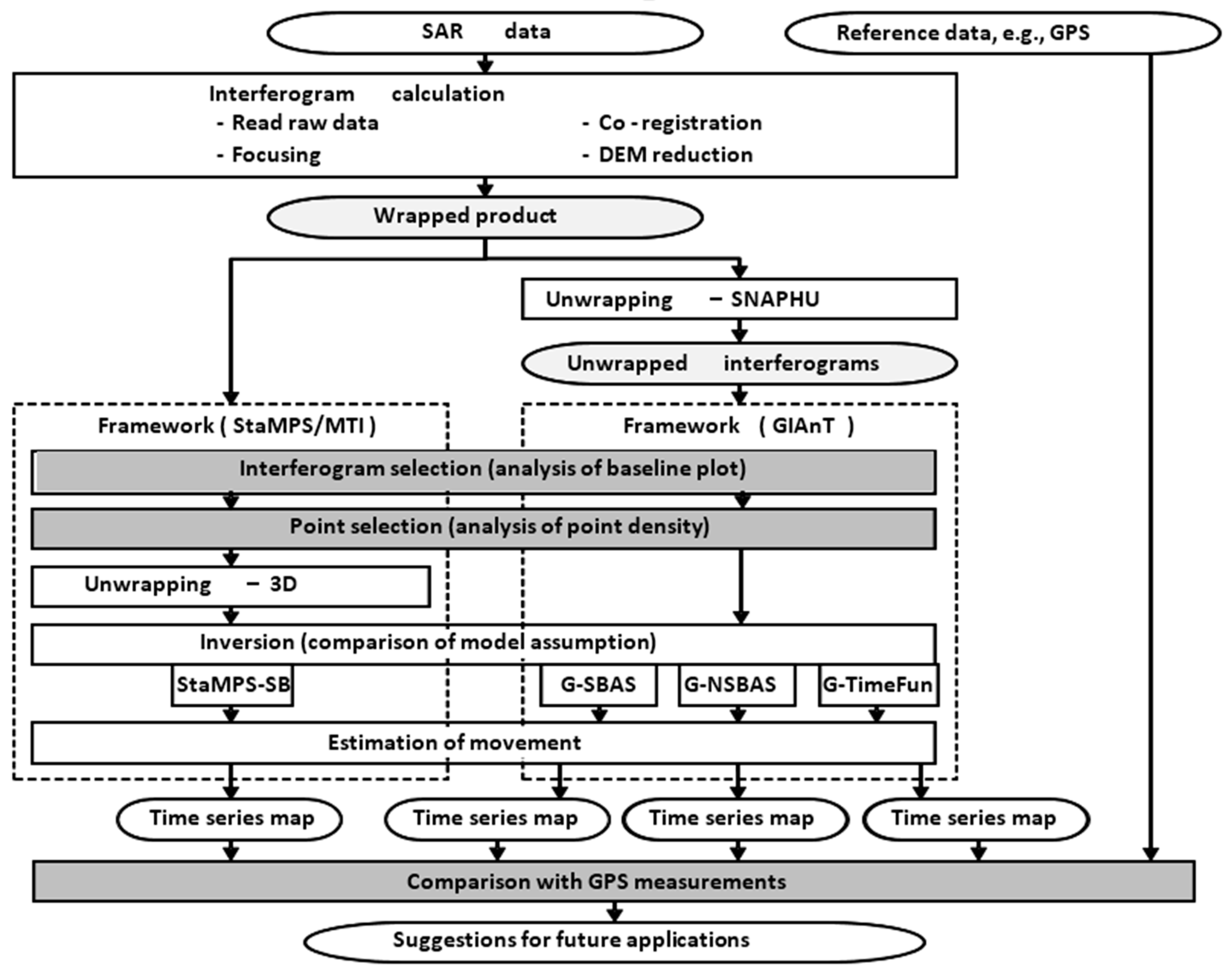
2. Theoretical Basis of Small-Baseline Interferometry Approaches

The general processing chain of SBI includes a pre-processing step to prepare small baseline differential interferograms followed by time series analysis. Figure 1 shows a demonstration of general work flow of the four analyzed SBI modules, from input SAR images to final products. The generation of differential interferograms follows the classical theory that has been very well explained in many previous reviews [34,35]. The processing steps that are the focus of this study are highlighted by rectangles filled with dark gray color.

2.1. Small-Baseline Interferogram Selection Criteria and Phase Unwrapping

The key point of the SBI analysis is to mitigate the impact of decorrelation by properly selecting the interferometric pairs with short temporal (B_t) and geometry (perpendicular, B_┴) baselines [17]. The maximum allowed baseline value is defined and used to constrain the interferogram pair selection. In order to avoid errors (e.g., phase unwrapping errors) propagating through the network of interferograms, it is also important to keep a sufficient number of redundant interferograms in the data stack [7]. This consideration needs to be kept in mind when constructing an optimal small baseline interferogram network. However, the interferogram time redundancy can be difficult to maintain for areas with low coherence and a limited number of SAR acquisitions. The Okmok site is a good example for limited data coverage and associated redundancy issues (Section 3). Note, that the connectivity requirement of interferogram networks also varies depending on the inversion scheme applied in different SBI approaches. The StaMPS-SB method requires that all interferograms are connected in one single subset [24] in order to use the classic Least-squares (LS) adjustment to determine the pixel phase at every individual SAR image. This is different to the seminal SBAS method [6] that can invert a small-baseline interferogram stack containing disconnect clusters by using a singular value decomposition (SVD) approach with a minimum-norm criterion. Similarly, the other three SBI implementations in GIAnT are also capable of inverting networks that are not fully connected. To this end, the methods employ an SVD approach and/or a predefined deformation model. In real data experiments (Section 3), in order to feed the four SBI modules with the same input data, the same stack of small baseline images containing no isolated clusters was constructed and applied for each test site.

Depending on the implemented unwrapping strategy, phase unwrapping may either be required prior to DSs selection (e.g., the three SBI implementations in the GIAnT toolbox) or can be applied after DSs were determined (e.g., StaMPS-SB). Nevertheless, the correctly unwrapped phase at every DS pixel is needed to generate displacement time series. Many phase unwrapping methods are focusing on processing a single interferogram (e.g., [36,37,38]); whereas, by jointly exploiting the spatio-temporal relationship of redundant interferogram stacks, three dimensional (3D) phase unwrapping methods (e.g., [39,40,41]) have been developed and have gained importance in multi-temporal interferogram processing. In our real data analyses, the 3D unwrapping algorithm [40] provided by StaMPS/MTI is used to solve the phase ambiguity at determined DS pixels for the StaMPS-SB solution. The two dimensional (2D) statistical-cost network-flow unwrapping algorithm, SNAPHU [36] is applied to prepare unwrapped phases for the three SBI modules in GIAnT. For the real data experiments in Section 3, the phase unwrapping step has been carefully conducted to ensure that all interferograms were unwrapped correctly. Also, GIAnT will provide tools to analyze the quality of inputted unwrapped interferograms in its future version.

2.2. Distribued Scatterer Pixel Selection

The DS pixels in StaMPS-SB are selected through an enhanced algorithm that is applied to the full resolution wrapped interferograms. The algorithm consists of two key steps: first, using amplitude difference dispersion [24], it selects an initial set of DS pixel candidates. This initial selection is done to reduce the computation effort for a subsequent down-selection step; second, the wrapped phase contribution${\varphi }^w$ at the individual DS candidates is split to three parts to compute decorrelation noise, ${\varphi }^w={\varphi }^c+{\varphi }^u+{\varphi }^n,$ namely a spatially-correlated contribution (${\varphi }^c$), a spatially-uncorrelated contribution (${\varphi }^u$) and decorrelation noise (${\varphi }^n$). ${\varphi }^c$ is estimated from surrounding pixels using a bandpass filter; ${\varphi }^u$, which is mostly terrain error-related, is modeled and estimated from its correlation with the perpendicular baseline. A subtraction of the computed ${\varphi }^c$ and ${\varphi }^u$ from ${\varphi }^w$ leaves ${\varphi }^n$, which is used to calculate the temporal coherence of the DS candidate. A threshold function of temporal coherence is used on ${\varphi }^n$ to finalize the DS identification in StaMPS-SB. The details of this algorithm have been well documented in previous publications [3,24].

For the other three SBI methods, the GIAnT toolbox implements a threshold selection based on standard spatial coherence of filtered and multi-looked interferograms. For both G-SBAS and G-TimeFun, only pixels with a coherence value above a single, user-specified threshold in all interferograms will be selected as DSs. Thus, G-SBAS and G-TimeFun share the same DS pixels.

For G-NSBAS processing, other than a single threshold on spatial coherence, another parameter that determines partially coherent pixels is used (described hereafter as a valid interferogram). Such pixels are coherent through parts of the interferometric time series. Thus, this option allows increased spatial coverage of DS points used in G-NSBAS, and the number of processed DS pixels in G-NSBAS may not be consistent among all SAR acquisitions. Additionally, a master image is selected as the temporal reference in G-NSBAS, because only those pixels that are coherent in at least one interferogram consisting of this temporal reference scene can be analyzed. Hence, to optimize the DS point coverage, this master image is expected to be able to compose coherent interferograms and have good connectivity with the rest of images. The maximum coverage of DS points in G-NSBAS will be used to compare the DS point coverage in G-SBAS/-Timefun and StaMPS-SB in Section 3.3, and to establish a discussion on the dependence of selection algorithms on the land cover type.

Other than the DSs identification methods in these four SBI modules, DSs can also be selected based on the temporal coherence calculated from adaptively filtered interferograms. To conduct adaptive filtering correctly, statistical tests are applied to find homogenous pixels from amplitude images beforehand [42,43]. This has been implemented in other multi-temporal interferometry techniques (e.g., SqueeSAR™ [11,44,45]); therefore, it will not be discussed in this paper.

2.3. Inversion of Interferograms to Individual SAR Scenes

For every selected DS pixel, the four processors invert small baseline interferometric phases from time series referencing to a single acquisition time. The primary idea of this step can be summarized as the linear operation shown in Equation (1).

$$\mathsf{\Phi }=D\cdot M$$

(1)

where $\mathsf{\Phi }$ is the vector of small-baseline phases, D is the design matrix, and M is the vector of model parameters to be retrieved. The formation of Equation (1) and the corresponding inversion strategy is one of the key steps in SBI analysis, although the exact content of D and M can vary for different SBI approaches. Assuming N single look complex (SLC) images, $\mathsf{\Gamma }$ interferograms, and following the notation used by [30], the main inversion schemes of the four SBI modules are summarized and compared in Equations (2)–(4).

$${\mathsf{\Phi }}_{mn}={\displaystyle {\displaystyle \sum }_{i=m}^{n-1}}\delta {\varphi }_i\forall \left(m,n\right)\in \mathsf{\Gamma }$$

(2)

Equation (2) is used in G-SBAS and StaMPS-SB to form the linear operator shown in Equation (1). ${\mathsf{\Phi }}_{mn}$ is the phase at a single pixel of a small-baseline interferogram consisting of SLCs m and n, and $\delta {\varphi }_i$ is the phase increment between the i and i+1 acquisition time that is to be estimated. A basic assumption here is that the deformation between time-adjacent unknowns is linear [6]. This inversion is repeated at every DS target that is coherent in all interferograms. With a fully connected interferogram network, StaMPS-SB solves the inversion with a classic LS adjustment [23,24]. This however, is not a pre-requisite for either G-SBAS or the other two modules, because an interferogram network with disconnected components can be solved via the SVD with minimum-norm constraints, or/and with assumptions based on a deformation temporal model.

$$\{\begin{array}{c}{\mathsf{\Phi }}_{mn}={\displaystyle {\displaystyle \sum }_{i=m}^{n-1}}\delta {\varphi }_i\text{ ∀}\left(m,n\right)\in \mathsf{\Gamma }(\mathrm{a})\\ 0=\gamma \cdot \left({\displaystyle {\displaystyle \sum }_{i=1}^{k-1}}\delta {\varphi }_i-f\left(t_k-t_0\right)\right)k\in \left[2,\text{N}\right](\mathrm{b})\end{array}$$

(3)

Equation (3) is used in G-NSBAS, where Equation (3a) is the same as Equation (2) and Equation (3b) is added as an extra constraint. $f(*)$ is the predefined parametric temporal deformation model, which is a function of the time difference between the acquisition k to the reference acquisition as $t_k-t_0$. To form the design matrix D in Equation (1) from Equation (3), $f(*)$ serves as a regularization function, and the contribution level of Equation (3b) is controlled by a weighting factor γ. Ideally, the setting of γ should depend on prior knowledge, e.g., (1) level of prior knowledge of the physical condition of the study area; (2) the number and degree of links of disconnected interferogram subsets; and (3) the number of SAR scenes and interferograms. Thus, G-NSBAS has more flexibility so as to process the interferograms with disconnected subsets and pixels that are not coherent in all interferograms. To processes pixels from disconnected interferogram subsets, it links the subsets through $f(*)$ (Equation (3b)); for pixels from complete small-baseline networks, a small γ can minimize the contribution from Equation (3b) and solve the inversion as a fit to the data. In this study, the default value (1e-4) of γ [30] is used for the LA test site and a value of 1 is used for the Okmok case (

Table 1. Specifications of Test Data and processing parameters.

Feature	Los Angeles (CA, USA)	Okmok (AK, USA)
Climate zone	subtropical zone	sub-arctic zone
Land cover	urban/forest/mountain	volcanic sediment/snow/scrubs
Deformation	periodical plus linear trend	none linear
SAR satellite	ERS-1/2	Envisat
Acquisition time	1995–2000	2003–2008
NO. of SLCs.	48	20
NO. of total IFGs.1	123	35
Coherence threshold (G-SBAS/Timefun)	0.1	0.1
Coherence threshold (G-NSBAS)	0.2	0.2
NO. of valid IFGs 1	105	30
γ	1 × 10−4	1
Gaussian filter length (year)	0.1	0.2

¹ IFGs. is short for Interferograms.

).

$${\mathsf{\Phi }}_{mn}={{\displaystyle \sum }}^{\text{}}{a}_u\left(f^u\left(t_m\right)-f^u\left(t_n\right)\right)\forall \left(m,n\right)\in \mathsf{\Gamma }$$

(4)

Equation (4) is used in G-TimeFun, where $t_m$ and $t_n$ are the SAR acquisition times; $f^u$ denotes a set of predefined deformation models, either parametric or interpolating functions; and $a_u$ are the corresponding coefficients in the model vector M of each pixel (Equation (1)). G-TimeFun applies the inversion with the minimization of regularized or non-regularized norm constraints defined by the user [30]. More mathematical details of these algorithms can be found in previously referred publications (e.g., [6,7,8,24]).

2.4. Mitigation of Non-Deformation Residuals

Non-deformation phase components, including atmospheric artifacts, topography-related errors and orbit errors need to be modeled and removed from the reconstructed time series phases to obtain the deformation history. The estimation of non-deformation terms, although mostly based on the same theory, can be done before, during, or after the inversion step, depending on the setting of each SBI algorithm. In the three modules from the GIAnT package, the orbital errors are modeled and subtracted as a spatial phase ramp from the small-baseline interferograms prior to inversion, through network deramping [25,28]; topographic errors can be modeled as a function of B_┴ that can be jointly estimated in the inversion step [30]. In StaMPS-SB, orbit errors can be modeled and subtracted as a spatial phase ramp from small-baseline interferograms independently; topographic errors, referred to as look-angle errors, are also modeled as a function of B_┴, both from small baseline interferograms and inverted single master interferograms, and are subtracted after the inversion step [18,40].

Both packages (STaMPS/MTI and GIAnT) contain extra modules to reduce atmospheric distortion signals, such as removing water vapor delays from the weather prediction model and estimating topography related atmospheric delays. However, we have only applied the atmospheric mitigation method within every SBI module in this study. The StaMPS-SB, G-SBAS and G-NSBAS modules reduce the residual atmospheric contribution by applying a spatial-temporal filter to the inverted time series with the expectation that the deformation signal is correlated in time, while artifacts (atmospheric signal and noise term) are not. In addition to the filter scheme, G-NSABS has the ability to reduce the atmospheric signal using a pre-defined deformation model in the inversion step. In G-TimeFun the atmospheric signal reduction is applied in the inversion step, as the estimation is fully constrained by user defined deformation functions.

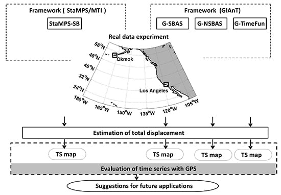
3. Real Data Experiment

In this section, we apply the SBI modules to the real dataset and evaluate their performance regarding the ground displacement reconstruction. The details of small-baseline interferogram selection and DSs targets selection are presented and discussed. The final displacement results are evaluated by comparing to the ground deformation measured by continuous Global Positioning System (GPS). The physical environment of the selected test sites, e.g., geophysical locations, ground coverage and deformation sources, are also introduced in this section.

3.1. Test Sites and Dataset

The LA and Okmok test sites have been chosen to assess the capability of the implemented SBI approaches to extract deformation signals under a variety of land coverage and topographical conditions. Figure 2 demonstrates the location of the study areas (large white rectangular areas in Figure 2a for the LA site and Figure 2b for the Okmok site) with their corresponding land cover types in the background. According to the National Land Cover Database (NLCD) [46] (see Figure 2), the LA test site is mostly urban with some vegetation, that is shrub and forest, while the Okmok site has only natural land cover types, including coverage of ice/snow, barren and herbaceous. The land cover type of each test site is also summarized in Table 1, together with temporal evolution conditions of deformation signals as suggested by previous studies [47,48], climate conditions, SAR data stack information, and the processing parameters with customized values at each test site that will be discussed in greater detail later. The GPS measurements [47,48,49] are used as references to assess the displacement results from different SBI modules, their locations are also shown as black circles in Figure 2 with Google Earth background [50].

3.1.1. Geodetic Setting of Study Areas and SAR Imagery

The deformation in the LA test site is composed of strong periodical and long-term vertical displacement, which is triggered by both tectonic and hydrogeological sources, e.g., displacement from fault zones and ground water usage [27,48,51,52,53]. The Okmok test site has a dominant deformation source from the underlying volcanic pressure system [54,55,56], but also contains localized surface subsidence in a limited region inside the caldera due to the contraction of a lava flow post-emplacement [54,57]. Previous studies [47,58] have suggested deformation signals prior to the Okmok eruption in 2008 were very non-linear.

In this study, we used SAR images of the LA test site acquired by the European Remote-Sensing satellites 1/2 (ERS 1/2) covering the period from 1995 April to 2000 December (48 SAR images). For the Okmok site we used SAR images acquired by Environmental Satellite (Envisat) spanning from 2003 June to several days before its eruption in July 2008 (20 SAR images). Both ERS 1/2 and Envisat had the same standard revisit period of 35 days. The temporal density of SAR acquisitions over the LA site is higher than for the Okmok test site. This is because (1) the ERS1/2 tandem setting was used at the LA site, which means some neighboring acquisitions have only a one day difference and (2) the SAR images of Okmok in the winter period were discarded due to their strong decorrelation in the high latitude region [55,59]. Thus, the SAR time series of the Okmok site contains large temporal gaps typically during the period from November to April. These large gaps in the data set have a strong impact on the temporal filtering processing that is implemented in many TS InSAR approaches and causes difficulties in recovering non-linear deformation signals [60]. In order to treat the individual SBI modules fairly, although it may not be the optimal solution in atmosphere mitigation, we have applied the same filter in the SBI implementations at each test site. Based on the previous geodetic results over these two sites [47,48], a Gaussian kernel filter with a standard deviation parameter of 0.1 years (approx. 37 days) for the LA site and 0.2 years (approx. 73 days) for the Okmok site (listed in Table 1) has been applied.

3.1.2. GPS Data at Test Sites

The reconstructed displacement time series from four SBI modules in the LA and Okmok areas will be compared to continuous GPS records. The locations of available GPS stations in the two test sites are indicated in Figure 2 with black circles. The continuous GPS sensors record position in time and are an important data source for geophysical research [61]. Moreover, previous research has demonstrated good consistency between the GPS and InSAR measurements at the LA site [48]. However, only five GPS stations (LEEP, HOLP, WHC1, LBC1 and LBC2) have sufficient time overlap with the ERS 1/2 SAR imagery at the LA site to be useful in the quantitative analysis. At the Okmok site, the geophysical products (that is, the volcanic source volume change) derived by the InSAR and GPS separately, are similar [47]. Thus, GPS measurements provide ideal reference data to evaluate the accuracy of reconstructed displacement history via different SBI approaches. The GPS data set for our Okmok case study is from Freymueller and Kaufman [58]. The GPS measurements of the LA site are part of the Southern California Integrated GPS Network (SCIGN) and are obtained from UNAVCO database [49]. GPS 3D movement measurements are projected to InSAR Line-of-sight (LOS) displacements for the comparison.

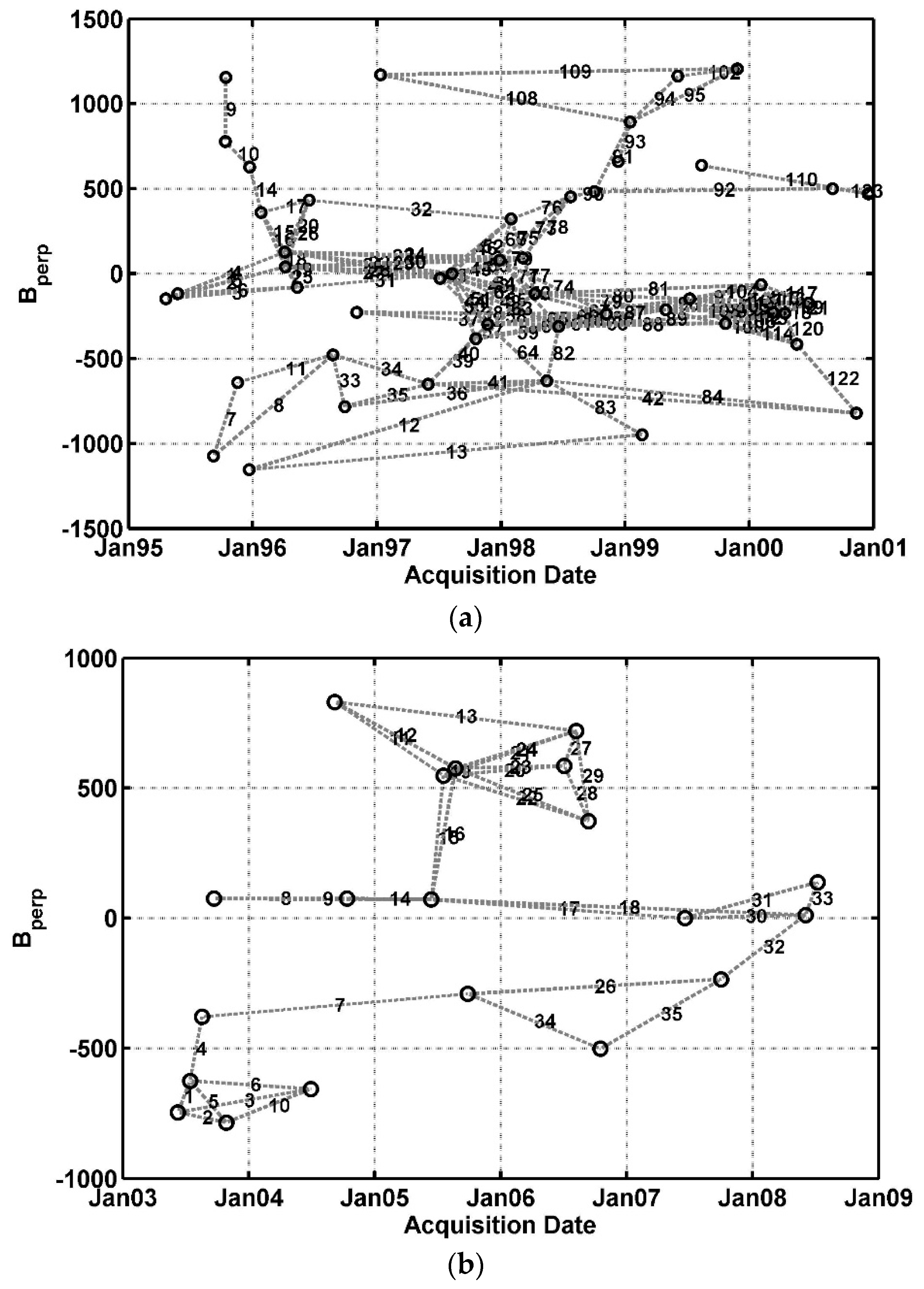
3.2. Small Baseline Interferograms Selection

In this study, an automatic interferogram selection has been applied to minimize the perpendicular (B_┴) and temporal (B_t) baselines, thus mitigating the decorrelation phenomenon. Its target is to include as many SAR images as possible in order to increase the sample size in the temporal domain. The two-step small baseline interferogram selection includes an initial selection prior to the interferogram generation based on coherence values predicted from SAR acquisition parameters, and a post selection based on the interferometric spatial coherence. In the initial selection, a threshold was set to include data pairs with predicted coherence (${\gamma }_s$) similar to that used in other studies (e.g., [4]). To predict the coherence for an interferogram with SLC index (m, n), we calculated ${\gamma }_s^{m,n}=g\left(B_{\perp }^{m,n},B_{\perp ,c}\right)\times g\left(B_T^{m,n},B_{T,c}\right)$, in which $B_{\perp ,c}$ is the critical perpendicular baseline and $B_{T,c}$ is the critical temporal baseline. This first pre-selection step allows us to only process data pairs that potentially have good coherence, for the sake of computational efficiency. The threshold of predicted coherence is set to 0.49 for the LA test site and 0.4 for the Okmok test site to maintain the complete connected network and to allow for a sufficient number of interferogram candidates for the second selection step. Due to the urban area coverage in the LA test site, $B_{T,c}$ is 5.5 years and $B_{\perp ,c}$ is 600 m so that 149 interferograms were generated after the initial selection. For the Okmok test site 87 interferograms were generated with $B_{T,c}$ of 3.5 years, given that there are fewer stable ground scatterers in natural environments than in urban regions, and $B_{\perp ,c}$ is 1 km due to the fact that geometry decorrelation was not observed to be the dominant decorrelation factor. The external Digital Elevation Model (DEM) from Shuttle Radar Topography Mission (SRTM) [62] and precise orbit vectors were used to reduce the topographic components and geometric contribution to the interferometric phase for both test sites.

The second selection is implemented on coherence maps to further reduce decorrelated interferograms while maintaining the connectivity of interferograms stack. The average spatial coherence was computed for every interferogram and those having low value have been discarded. After the second selection, 123 interferograms for the LA test site and 35 interferograms for the Okmok test site remain. The time-baseline plots for the two test sites are shown in Figure 3.

As mentioned before, an optimal small baseline interferogram stack also needs sufficient time redundancy to avoid error propagation through the network inversion. However, the Okmok site has a weak network with limited redundant interferograms in time, because of the poor coherence characteristics of the study area. For instance, as shown in Figure 3b interferograms with index number 4, 7, 32 connect different interferogram subsets but are not belonging to a closed loop. Thus, any existing error will propagate in the retrieved displacement time series and the error level of reconstructed deformation signals at Okmok test site is supposed to be larger than that at LA test site.

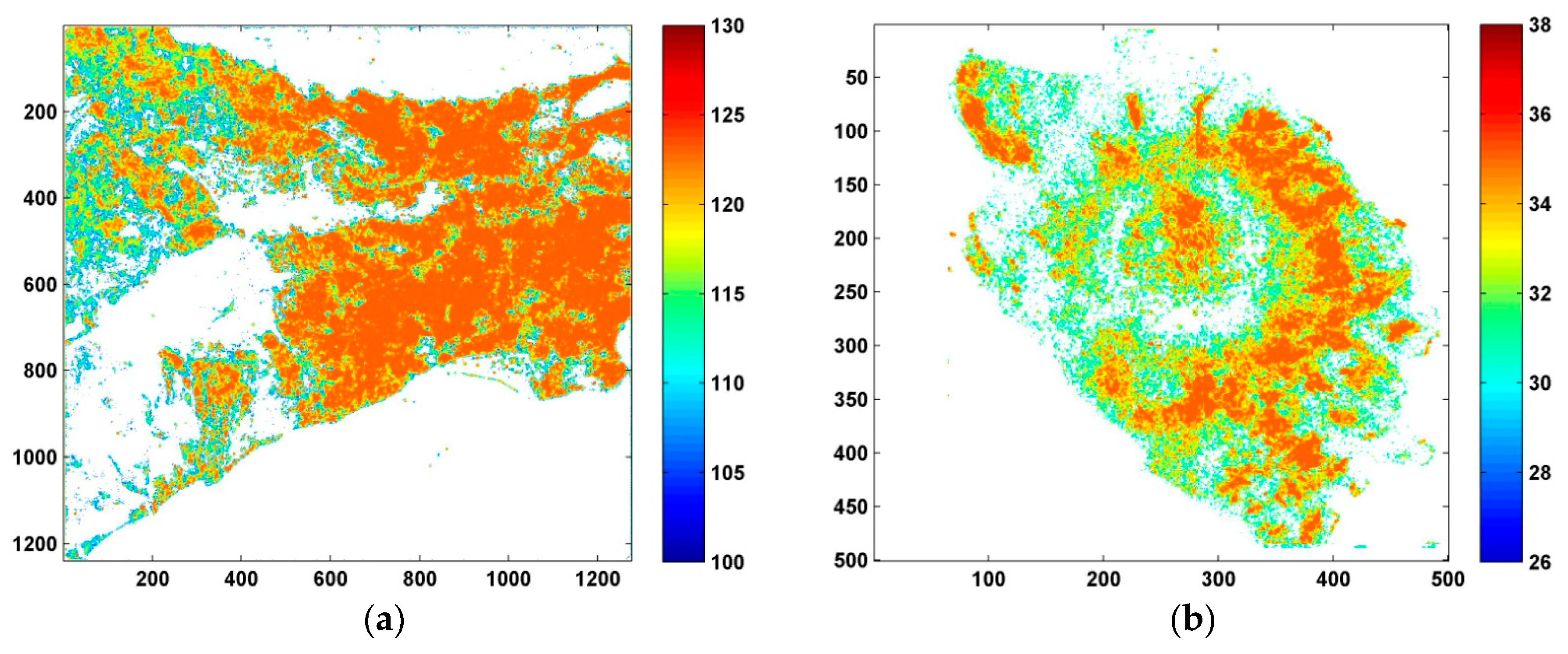
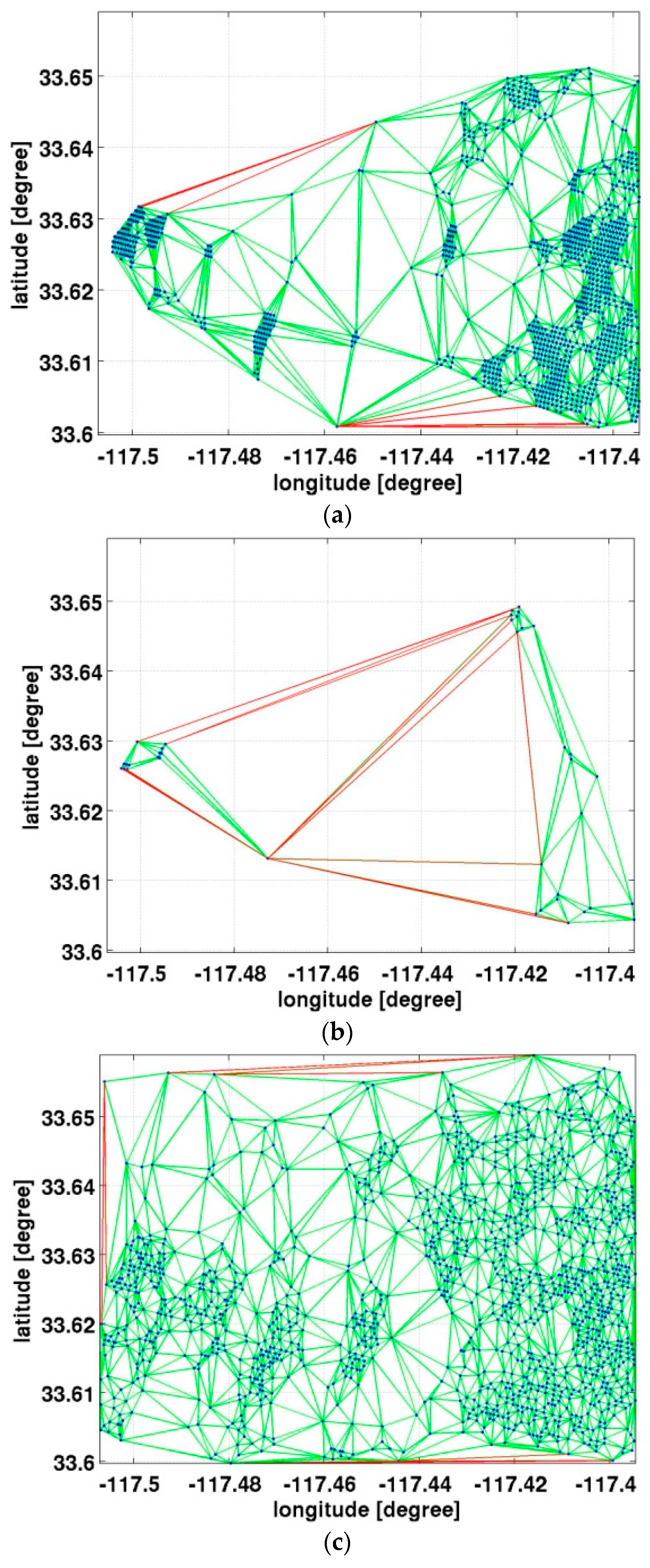
3.3. DS Point Selection and Coverage Evaluation

In this section, a quantitative analysis on the spatial coverage of DS targets from different DS selection strategies is presented. As mentioned earlier, the StaMPS-SB processes full resolution interferograms, while the interferograms used in the GIAnT toolbox are multi-looked with factor 4 in range and 20 in azimuth for both two test sites. To initiate a discussion on the achieved DS point coverage, StaMPS-SB results are re-gridded into the same multi-looked frame prior to the comparison being made.

The suggested threshold values for StaMPS-SB pixel selection are used here, where the threshold of amplitude difference dispersion is 0.6, and maximum acceptable spatial density of identified pixel with random phase is 2 per km². The spatial coherence threshold value used in G-TimeFun and G-SBAS for DS pixels selection is 0.10 for both the LA and Okmok test sites as listed in Table 1, corresponding to an interferometric phase standard deviation of less than 80 degree when using 20 independent looks [16,63]. This threshold value is lower than the suggested setting, e.g., fixing the coherence threshold of 0.25 [6]. This is in order to obtain enough coverage so comparisons could be made to GPS records. The choice of this threshold also considers the bias in coherence estimation [34]. By computing the coherence value from open water areas in both sites, we find pixels with coherence values less than 0.08 can be regarded as fully decorrelated.

The coherence threshold for selecting the pixels used in G-NSBAS is larger than that for G-SBAS and G-TimeFun, given G-NSBAS can process temporarily coherent pixels. The choice of coherence thresholds for G-NSBAS is suggested to balance the DS ground coverage with the capability of algorithm [30]. Here, we choose a value of 0.2 for the two sites (

Table 2. DS point density and spatial distribution analysis.

Site Name	SBAS Method	Point Density (DS/km2)	Coverage Ratio (km2) 1	σ Triangle Size (km2) 2	Short Arc. Median (km)
OK Ice/Snow and scrub	G-NSABS	53.50	0.73	97.02	0.09
	G-SBAS G-TimeFun	34.01	0.71	112.47	0.10
	StaMPS-SB 3	12.07	0.72	226.47	0.16
LA-1 Forest and Scrub	G-NSABS	15.63	0.61	86.80	0.09
	G-SBAS G-TimeFun	0.55	0.43	1602.80	0.39
	StaMPS-SB 3	19.68	0.95	58.67	0.17
LA-2 Developed, low to medium intensity and open space	G-NSABS	162.26	0.99	0.76	0.08
	G-SBAS G-TimeFun	134.54	0.99	4.69	0.08
	StaMPS-SB 3	89.13	0.99	3.43	0.11
LA-3	G-NSABS	163.63	1.00	2.07	0.08
Developed, medium to high intensity	G-SBAS G-TimeFun	119.69	0.99	7.39	0.08
	StaMPS-SB 3	91.72	1.00	3.08	0.11

¹ The coverage ratio is computed as the size of the area covered by the triangulation network divided by the size of the subset; ² Standard deviation (σ) of the size of the triangles in the network; ³ the point density of StaMPS-SB is calculated after resampling.

), also smaller than the suggested default value. The second DSs selection parameter in G-NSBAS, number of valid interferograms, is set up to collect pixels that are coherent in more than 85% of all interferograms. For both cases, the first acquisition is selected as master, which is connected to the other SAR images through coherent interferograms. Again, the number of DS pixels processed in G-NSBAS is not consistent among all interferograms and the maximum point coverage is used in the DS coverage analysis. The number of interferograms used in G-NSBAS for every pixel of two test sites is displayed in Figure 4. At the LA test site, most of pixels were processed with 123 interferograms, with a fully connected network, while the partially coherent pixels that mostly sit in the mountain/vegetation region have a minimum of 105 interferograms. For the Okmok case, the maximum number of interferograms used is 35, and the minimum requirement is 30. Overall, three sets of DS targets are used in the time series analysis with StaMPS-SB, G-SBAS/G-TimeFun and G-NSBAS respectively, and are compared below.

Three sub-sites in the LA test area were selected in order to include all the major land cover types in this area. These sub-sites are denoted by smaller boxes shown in Figure 2, while the Okmok site was analyzed in one piece. The LA sub-sites include the subset-1 covered by forest and scrub lands, subset-2 containing low to medium developed areas and developed open space and subset-3 contains medium to high intensity developed area. The land cover of the Okmok area is less complex with mostly ice or snow and scrubs, so the full area is analyzed.

The density of coherent points is commonly used in analyses of selected DS targets. However, it can only provide limited knowledge on the spatial distribution of targets. The spatial distribution of DS pixels is also vital in the deformation field reconstruction in order to provide full control over the study area. We built Delaunay networks to analyze the spatial distribution of DS pixels selected from different algorithms, an approach similar to the previous study in [64]. The evaluation parameters are listed in Table 2, including the average DS point density within every subset, the median length of arcs shorter than 3 km (short arcs for short hereafter), the size-ratio of the Delaunay triangulation network coverage to the subset size (coverage ratio for short hereafter) and the size standard deviation of triangles (tri. σ for short hereafter). Given arcs with large distances are not preferred as they are related to isolated DS clusters and holes in DS points coverage, the median distance of short arcs implies the general arc distance of pixel pairs that are favored in triangulation networks. Another parameter, the coverage ratio, is used to demonstrate the capability of each DS selection algorithm to have enough points to cover the full subset. The last parameter discussed here, the tri. σ, is used to indicate the distribution of triangle size within the subset. For instance, in a dense and evenly distributed network, the tri. σ is expected to be small whereas with sparely distrusted DS clusters that are connected with long arcs, the tri. σ will be large.

An example of point distributions for LA subset-1 is visualized in Figure 5, which demonstrates how the spatial distribution of DS points is related to the evaluation parameters listed in Table 2. This subset is mostly covered by forest and scrubs hampering the long-term spatial coherence and leading to low point density of less than 1 DS/km² (Table 2) if the single parameter coherence threshold for G-SBAS and G-TimeFun is used. There are more DS pixels in G-NSBAS, and StaMPS-SB is able to extract the greatest number of DS pixels. As shown in Figure 5a, there are several clusters of DS points for the G-NSBAS module, and its network coverage is not able to cover the whole subset. In the same subset, only the DS points for StaMPS-SB provide reasonable coverage for the whole area. Even though the full subset area is partially covered by the triangular network, the points selected in the G-NSBAS module are better spatially distributed than the DS points of G-SBAS/G-TimeFun as indicated by the values for tri. σ and the median distance of short arcs of 0.09 km, both listed in Table 2.

For the other two subsets over urban regions, all three selection strategies are able to fully cover the subsets (as shown by the coverage ratio of about 1) and show similar spatial distributions with median distances of short arcs being 0.08 km–0.11 km and tri. σ less than 8 km². The DS density in StaMPS-SB is smaller than that of the other two schemes, whereas the DS distribution in G-SBAS/G-TimeFun has larger tri. σ value, indicating less even point distribution.

As expected at the Okmok site, DS points are less dense than in the urban areas of LA, as shown by smaller point density value and larger tri. σ values. DS points produced by G-NSBAS show the best spatial coverage. The relatively low coverage ratio value of all compared algorithms at this site is due to the surrounding ocean. As mentioned above, the coherence thresholds used in the three modules of the GIAnT package are lower than the suggested values, while the default setup of the enhanced coherence estimation technique is used in StaMPS-SB. Under the same conditions, DS points in the StaMPS-SB module have maintained the comparable spatial coverage and shown better performance in the LA subset-1. Although DS point coverage of StaMPS-SB is not as high as the other three modules in the Okmok case, we can expect an improvement of spatial coverage by slightly relaxing its selection criteria.

Overall, with the current threshold setting, all three point selection strategies are able to provide sufficient DS coverage, especially a reasonably dense network in urban areas such as LA subsets 2 and 3; the performance of StaMPS-SB is better in the mid-latitude non-urban area with forest and scrub and DS points produced by G-NSBAS have demonstrated the highest point density in most cases.

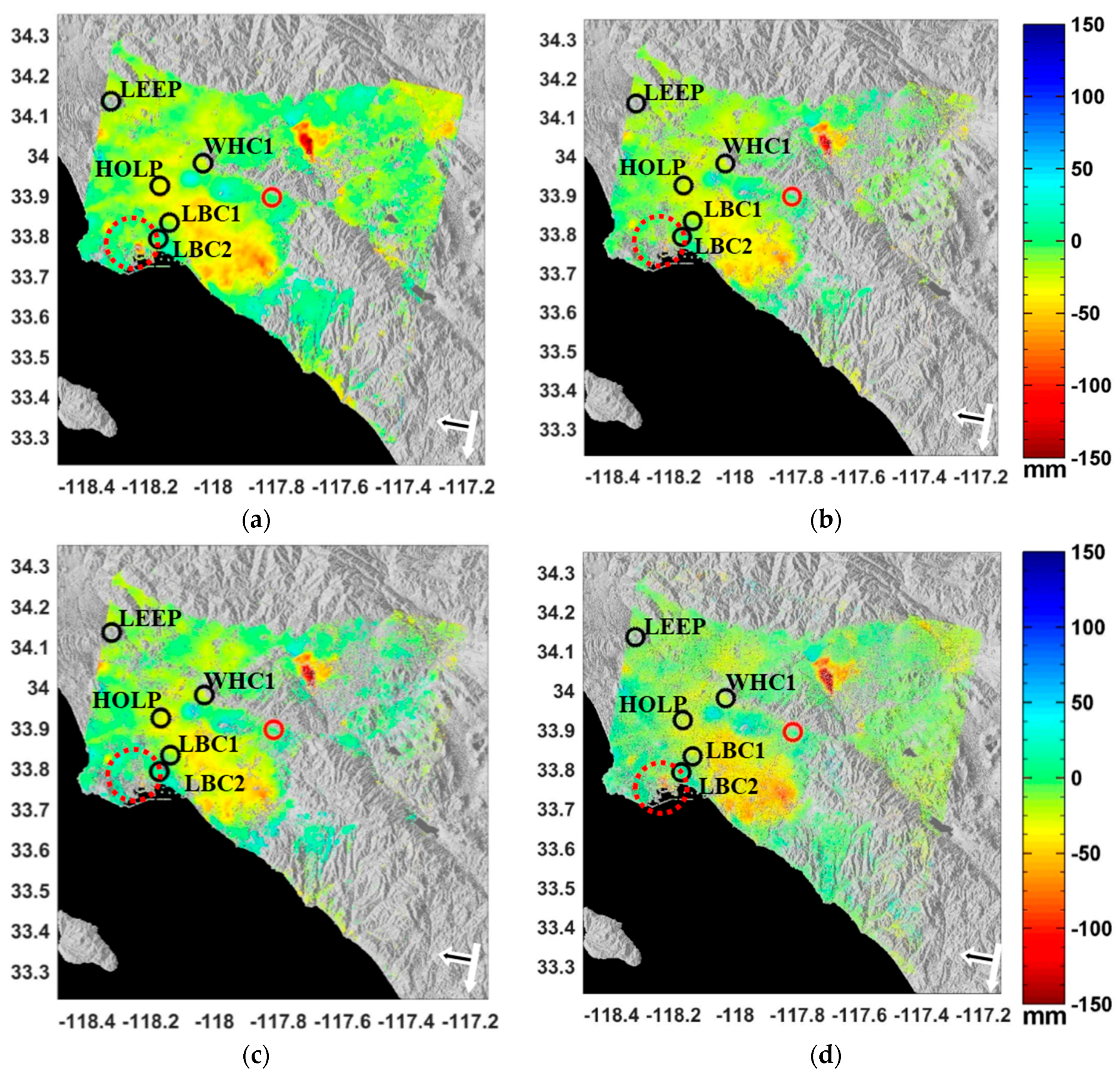
3.4. Estimation of Surface Deformation

As the primary purpose of SBI techniques is to reconstruct the ground deformation history, this subsection will compare the deformation time series extracted from the four SBI modules to GPS records. The 3D GPS measurements were projected to InSAR LOS movements based on the known satellite geometry parameters, including satellite heading angle and incidence angle and movement towards the satellite is defined as positive. The 3D position standard deviations in the GPS records are also converted to the corresponding errors in LOS direction through error propagation.

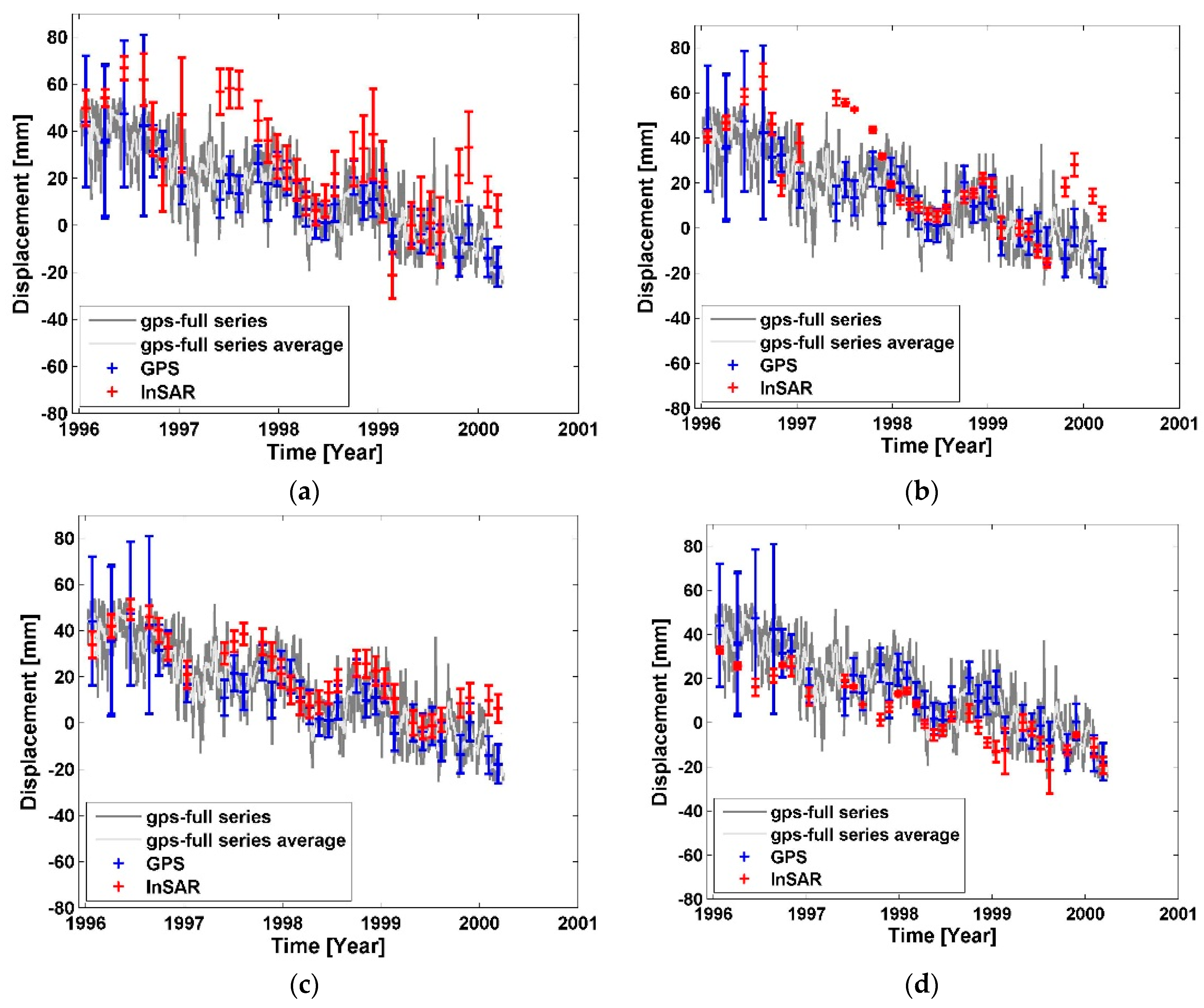
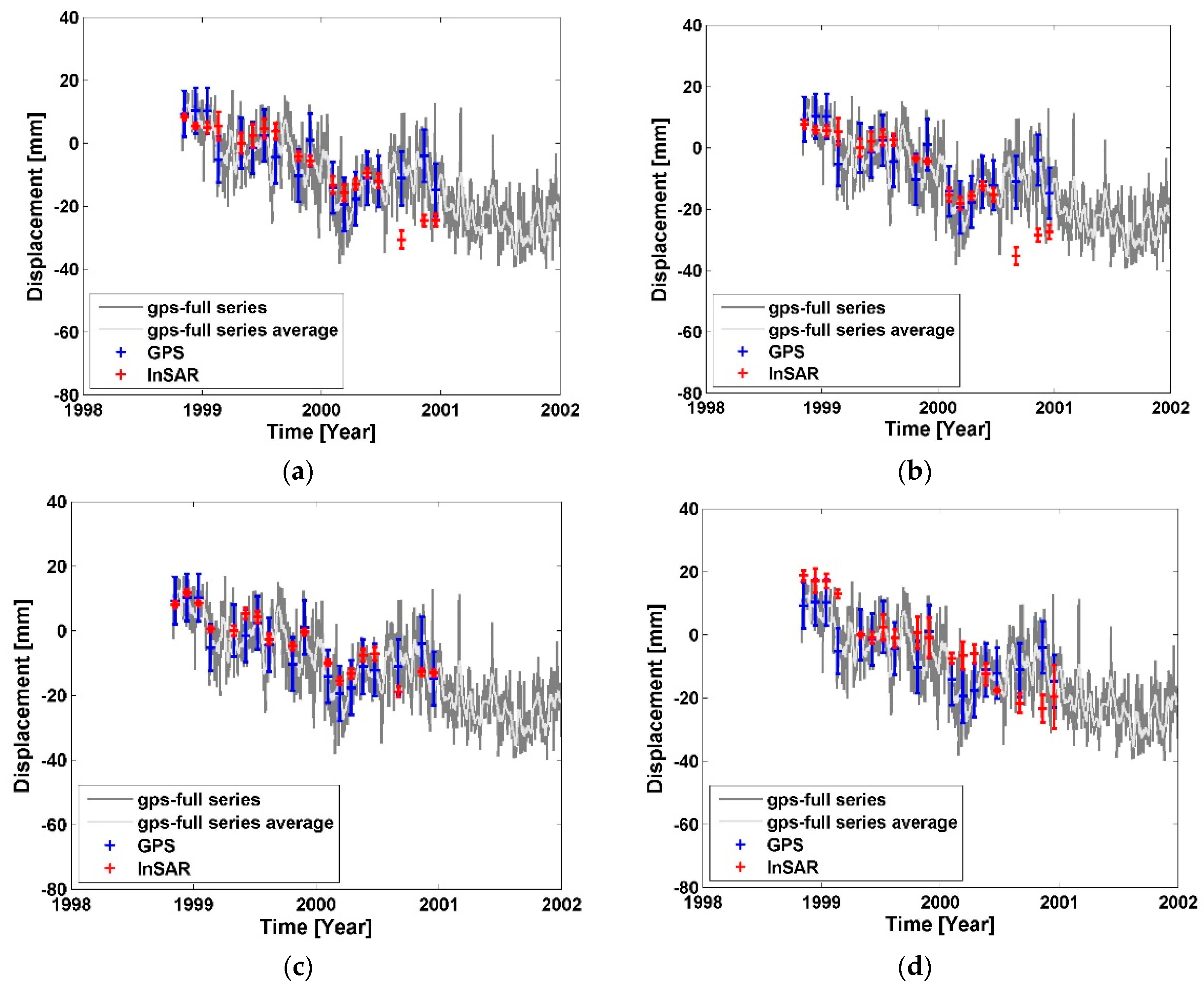
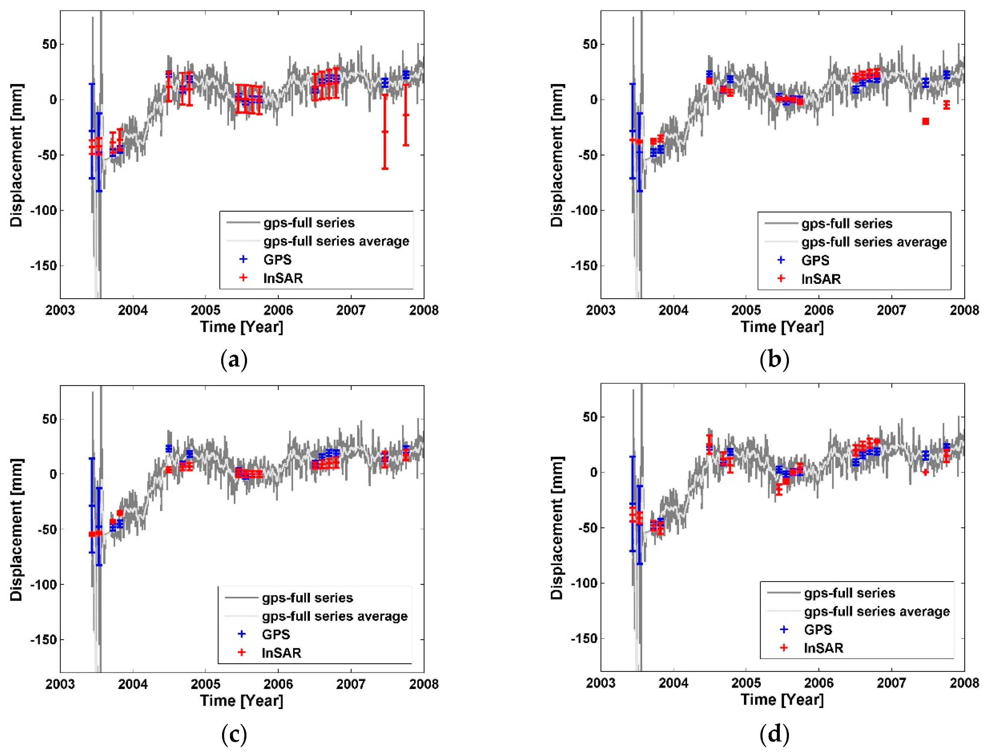
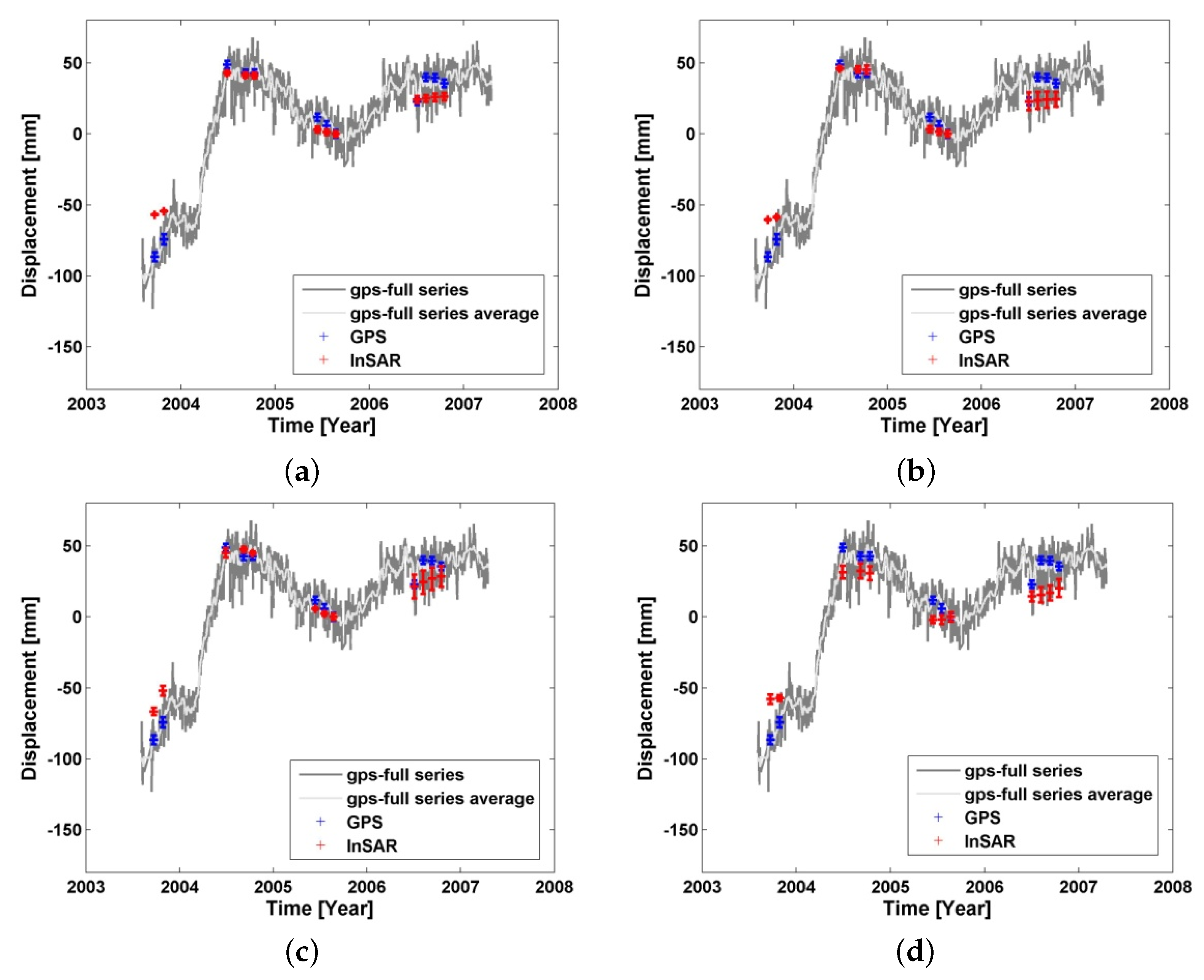
3.4.1. Comparison of Small Baseline InSAR and GPS Measurements for the LA Site

Given the previously suggested strong periodical ground deformation in the Los Angeles Basin [27,48,51,52,53,65], a temporal evolution model consisting of periodic and linear functions has been used in G-TimeFun and G-NSBAS modules. To demonstrate the results, the total displacement fields for the period 1995–2000 generated by the four SBI approaches are shown in Figure 6. The displacement maps have the same spatial reference denoted by the red marker in the figures so that they are comparable with each other. The figures show similar deforming patterns, although the G-NSBAS result seems smoother because of its higher point density. A region circled by the red dashed lines in Figure 6 is a previously suggested deforming area [27], however it is only retrieved by G-NSBAS and StaMPS-SB approaches, likely due to their better point coverage in this region.

There are several GPS sites in the SAR image frame (shown in Figure 2a by black circles) of the LA site, however many of them are lacking sufficient temporal overlap with the SAR image time series. Thus, five of them, namely, LEEP, HOLP, WHC1, LBC1 and LBC2, which contain observations before 1999, are used in this study. The GPS records are stored in the UNAVCO database and can be freely accessed [49]. The temporal reference of both the GPS and SAR products is set to be 1 May 1999. The differential displacement between two GPS sites (referred as displacement arc hereafter) are computed and compared to the equivalent measurement derived from the SBI processors in order to overcome the different spatial reference in the InSAR and GPS systems. Differential displacement measurements are plotted in Figure 7, Figure 8 and Figure 9, which correspond to the displacement arcs LEEP-HOLP, WHC1-LEEP and LBC2-LBC1. The displacements at arcs are formed as displacement at point1 minus that at point2 (denoted as point1—point2). In this form, the measurement at point2 is used as a reference of each arc, and its uncertainty is not propagated into the error bounds of differential displacement measurements at the arc. Thus it can better demonstrate the quality of SBI results especially at point1 in every arc.

In Figure 7, Figure 8 and Figure 9 the daily GPS measurement (including the daily position solution and associate uncertainty) in the LOS direction of the arc is denoted by dark gray lines. The GPS measurements have also been smoothed via a five-day moving window filter to reduce the temporal random noise (light gray lines), and the average measurements at the same SAR image acquisition dates are highlighted by blue dots with error bars.

To initiate a comparison, the DS targets close to every GPS site are selected adaptively to maintain an average distance between the GPS site and DS points of less than 800 m and with a minimum of 3 DS points selected in order to guarantee they are recording the same ground deformation. The standard deviation of displacements of selected DS pixels is computed and used as the corresponding error bounds (red markers) at every SAR acquisition time. In this way, the error bounds account mainly for uncorrelated spatial noise in the retrieved deformation time series (e.g., decorrelation and local unwrapping errors) by assuming nearby scatterers have similar deformation histories. However, spatially correlated residuals (e.g., atmospheric errors) may not be included and are expected to be largely mitigated in SBI analysis. The SBI derived displacements are denoted by red dots with error bars and are plotted separately in the figures regarding their corresponding SBI processor. In

Table 3. Comparison of GPS and SBAS results for LA test site.

Arc 1		Method	Mean Distance 2 (m)		Residual 3 (mm)
Point 1	Point 2		Point 1	Point 2	Offset	σ
LEEP	HOLP	G-NSBAS	572.72	32.95	−15.42	14.95
		G-SBAS	758.32	71.46	−10.57	15.27
		G-TimeFun	758.32	71.46	−8.09	8.96
		StaMPS-SB	144.00	70.68	8.74	8.81
WHC1	LEEP	G-NSBAS	42.27	572.72	0.86	7.24
		G-SBAS	42.27	758.32	−1.27	8.41
		G-TimeFun	42.27	758.32	−1.21	7.44
		StaMPS-SB	59.07	144.00	−2.78	8.46
LBC2	LBC1	G-NSBAS	49.33	31.88	1.40	8.53
		G-SBAS	49.33	31.88	2.82	9.42
		G-TimeFun	49.33	31.88	−1.40	4.35
		StaMPS-SB	59.40	58.51	−2.43	9.17

¹ The differential displacement at every arc is computed as point1 minus point2; ² the mean distance of selected DS points to GPS site location; ³ the residual time series is computed as GPS minus SBAS and σ is the acronym for standard deviation; offset is the mean value of the residual indicating the bias in the estimation. The same notation is used in Table 4.

, the average distance of selected DS points to nearby GPS sites for every method is listed. As shown in Figure 7, Figure 8 and Figure 9, all four SBI processors are able to capture the major linear deformation trend, while the quality of reconstructed seasonal deformation varies from case to case. Note that the temporal sampling rate of 35 days of the input ERS data is theoretically sufficient to capture the seasonal deformation in this area, but data gaps and high noise level would introduce difficulties. Taking arc WHC1-LEEP as an example (Figure 8), the peak-to-peak periodical displacement is relatively low, which means recovered deformation time series have underestimated the non-linear components. The statistics of the time series differences between GPS and SBI results at common acquisition time of every arc are computed and listed in Table 3, including the residual mean value (offset) and standard deviation (σ).

In Figure 7, the overall relative subsiding trend between LEEP and HOLP has been captured. The shape of G-NSBAS time series at this arc looks mostly similar to that from G-SBAS, while the reconstructed time series from G-NSBAS contains relative larger errors. This is because the weight factor (γ) in G-NSBAS of LA site is 1 × 10⁻⁴, so that the impact of the previous defined deformation model is small when points have complete network. Given that HOLP is used as a reference, the error bound of the arc is contributed by SBI measurements around the LEEP station only. Such errors could be the result of phase unwrapping errors (specifically in the unwrapped interferograms feeding GIAnT modules) at points around LEEP that compromise the time series inversion. StaMPS-SB is able to retrieve a less noisy time series, which is likely due to the 3D unwrapping algorithm applied in the module. As shown in Table 3, the average distance of points nearby LEEP used in G-NSBAS of 572.72 m is smaller than that in G-SBAS/G-TimeFun of 758.32 m that implies different point coverage in G-NSBAS. Thus, although G-NSBAS has a better point coverage around LEEP, it likely includes some points with inconsistent qualities that contribute to the large error bounds. At the same arc, DS targets selected by StaMPS-SB are closer to LEEP with an average distance of 144 m and have produced results with smaller residual (Table 3). Note that in Figure 2, the land cover type around LEEP is scrub and developed open space, thus the comparison suggests that the DS target selection and deformation extraction applied in StaMPS-SB performed better in this natural environment. Although G-SBAS and G-TimeFun solutions are based on the same pixels, the solution from G-TimeFun is constrained by the given deformation model library. Comparing the result residual (Table 3), it indicates the G-TimeFun result agrees better with the GPS measurements than the G-SBAS result at all three arcs. Additionally, at arc LBC2-LBC1, the three modules G-SBAS, G-TimeFun and G-NSBAS have processed the same DS pixels, however have produced time series results with different quality. This is largely due to the impact of the deformation model constraint. Theoretically, applying a weight factor with larger value in G-NSBAS to increase the impact of the temporal deformation model may achieve a result similar to that from G-TimeFun. Overall, the agreement between the SBI reconstructed displacement time series and the GPS measurements is mostly better than 10 mm.

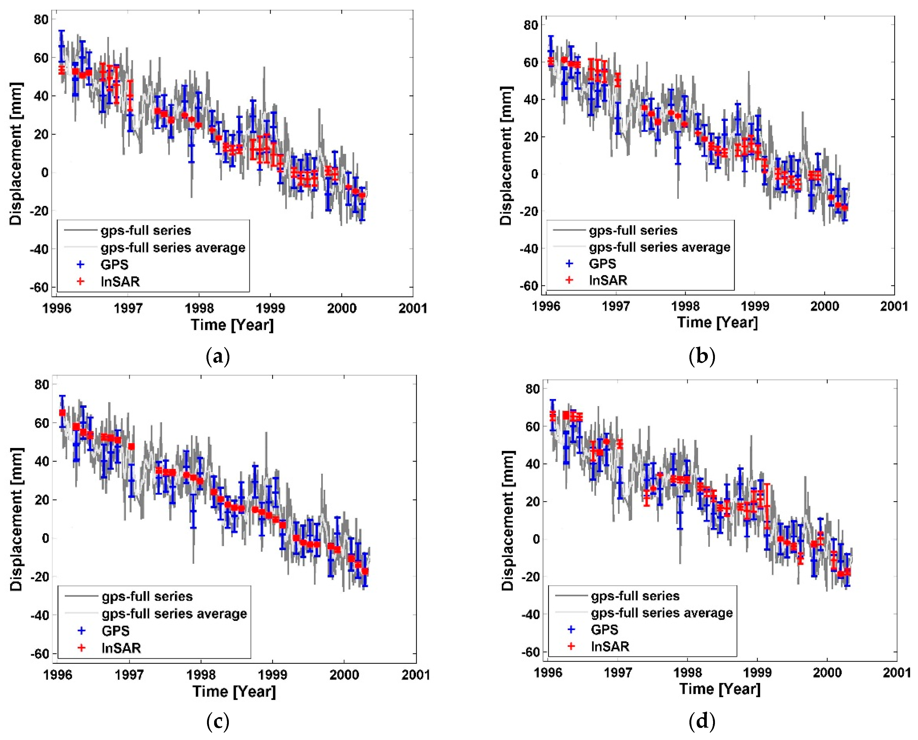
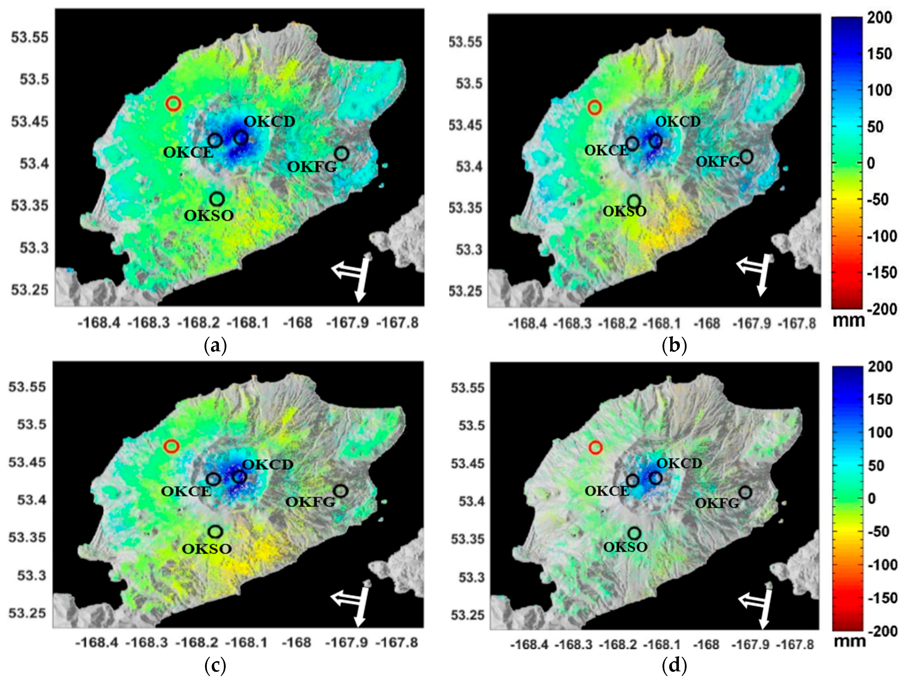
3.4.2. Comparison of Small Baseline InSAR and GPS Measurements for the Okmok Site

A similar comparison between the GPS and SBI displacement products was conducted for the Okmok test site. The deformation in the Okmok site was suggested to be non-linear and irregular [47], thus in this case, a 7th order polynomial deformation model is given for the G-TimeFun and G-NSBAS approaches, and γ has a value of 1 in this case to emphasis the constraint from the predefined deformation model in G-NSBAS.

The total displacement field of the Okmok Volcano derived from the four modules for the period 2003–2008 is plotted in Figure 10. The main deformation is the pre-eruption inflation of the underlying volcanic source. Additionally, there are two areas in the center of the caldera impacted by volcanic flow emplacement processes [57,66]. Despite this complex deformation condition and despite the sparse sampling with SAR data in time, all four SBI modules are able to capture the deformation signal at these two flow deposit regions indicated by the light blue color at the south-western region in the caldera, and the other one closer to the caldera center. Also, the results agree with each other with regard to the captured volcanic inflation pattern.

As shown in Figure 2b, all the GPS stations after 2000 are denoted by black circles. The majority of the GPS stations in Okmok are campaign sites with only four continuous GPS sites that have sufficient temporal overlap with processed SAR data: OKFG, OKCE, OKSO and OKCD. Both OKCD and OKCE were sitting inside the Okmok caldera ring and had hardware failure in/after 2007 [58]. Moreover, OKCE has large position variances in 2002–2003 due to instrument issue [47]. OKSO and OKFG were located outside the caldera ring and therefore less affected by volcanic deformation; only few relative deformation signals between OKSO and OKFG during the 2003–2008 timeframe have been found. Thus, two arcs were used for the differential displacement analysis here, OKCE–OKFG shown in Figure 11 and OKCD-OKSO shown in Figure 12. Both of them are referenced to 23 August 2005. Again, the DS points are selected adaptively around the GPS site location with the same setting used in the LA site.

Both these two arcs show non-linear deformation signals. At site OKCE, all applied modules are able to capture the main displacement increment from 2004 to 2005. The result from G-TimeFun seems smooth in time compared to the other solutions and it underestimates the uplift peak in 2005. The results from G-NSBAS, G-SBAS and StaMPS-SB have in common that the two records in 2007 shift away from GPS average measurements, which might be caused by temporal gaps in data set and artifacts in these two acquisitions. The G-NSBAS measurements around OKCE site are not consistent, leading to larger error bars, especially at the two records in 2007. At this example, the DS points used in StaMPS-SB are located relatively further away from the OKFG site, while residual standard deviation (σ) of differential displacement recovered by the StaMPS-SB is similar to that of G-TimeFun as shown in

Table 4. Comparison of GPS and SBAS results for Okmok test site.

Arc		Method	Mean Distance [m]		Residual [mm]
Point 1	Point 2		Point 1	Point 2	Offset	σ
OKCE	OKFG	G-NSBAS	196.75	145.68	5.92	14.47
		G-SBAS	196.72	224.00	1.91	12.92
		G-TimeFun	196.72	224.00	4.77	8.57
		StaMPS-SB	168.35	453.61	1.37	9.00
OKCD	OKSO	G-NSBAS	58.41	72.84	0.77	13.20
		G-SBAS	88.88	72.84	0.96	12.32
		G-TimeFun	88.88	72.84	0.04	11.42
		StaMPS-SB	112.32	123.57	7.18	15.68

. The larger residual offsets of G-TimeFun and G-NSBAS results indicate an existing bias in the measurements, which could stem from the estimation at the temporal reference date.

There is significant non-linear deformation at site OKCD. The major displacement peaks have been recovered by all tested SBI approaches as shown in Figure 12. In this example, the main disagreement between GPS and InSAR records are from the acquisitions in 2003. Due to the temporal gaps in the data set and sparse samples per year, it is difficult for the implemented small baseline modules to reproduce the intra-annual displacement changes. As shown in Table 4, the result from G-TimeFun at OKCD-OKSO has smaller residuals, suggesting that G-TimeFun with a predefined deformation model constraint could improve the result quality. Overall, the residuals between SBI modules and GPS measurements at the point-arcs of the Okmok case have a standard deviation of 8–16 mm. The overall residual level is larger than that in the LA case, which is due to the natural environment, limited redundant interferograms in time, acquisition gaps, and less regular non-deformation signals at Okmok Volcano.

4. Discussion

Based on the analysis of the DS point coverage and the quality of geodetic results from the four SBI modules, conclusions regarding their strengths and limitations are as follows:

The four SBI processors are all capable of providing a ground deformation time series analysis. When applying the processor to the urban area with a proper temporal sampling of SAR acquisitions, they have shown mostly similar performance and results. The application with a large acquisition gap in the data set and non-linear deformation needs to be carefully conducted. For such difficult case studies, an optimal small-baseline interferograms stack with high interferogram redundancy in time is preferred in order to reduce error impacts on the inversion step. A predefined deformation model, if available, provides solutions with better constraints, e.g., SBI modules G-NSBAS and G-TimeFun could improve the quality of the time series result. Otherwise, the model-free SBI approach, StaMPS-SB, is also a good choice that preserves the non-linear deformation signal and produces measurements with good spatial coverage especially in natural environments. This study has mostly used the default settings of processing parameters suggested by those SBI modules, the optimization of these parameter values may vary case by case, hence is not discussed here. Both StaMPS/MTI and GIAnT packages provide extra atmospheric correction modules, which can be applied depending on the external atmospheric data availability and topography condition. However, given they are separated from the main SBI modules, only the phase-based atmospheric correction schemes in SBI modules have been applied.

The quality and coverage of the selected DS points is important to all four SBI processors. Spatial coherence thresholding schemes were used in the GIAnT package. In the StaMPS/MTI package, enhanced temporal coherence and amplitude difference dispersion analysis have been used in DSs identification. The selection methods with a single spatial coherence threshold for G-SBAS and G-TimeFun have encountered difficulties in handling areas with natural features in the LA test case. Note that for modules in GIAnT, we have reduced spatial coherence thresholds rather than using the default setting in order to have enough DS points around GPS sites. For similar applications, we do not suggest coherence threshold values below the setting presented in this study for GIAnT modules, because it will include decorrelated pixels and lead to noisy results. For applications containing natural environments, we favor StaMPS-SB with the enhanced coherence technique, especially in case of prior geodetic information not being available, as this technique could reduce large spatial holes in DSs coverage over non-urbanized region. We also recommend the G-NSBAS module, if prior knowledge about the shape of the temporal deformation model is available, as it could achieve higher DS point densities given a proper setup of the number of valid interferograms and the master image. Note that the SBI modules in the GIAnT toolbox are able to process small-baseline interferogram stacks with incomplete networks. Theoretically, this could improve the DS point spatial coverage because interferograms with low coherence can be discarded rather than be processed to maintain network connectivity. However, this choice is not discussed in this study in order to conduct the fair comparison among four modules.

To successfully conduct inversion with G-NSBAS and G-TimeFun, valid assumptions about the temporal deformation model are needed. The predefined model needs to describe the temporal behavior of all types of deformation signals sufficiently, which can be a summation of functions for different deformation signals in the study area. Note that one of the benefits of deformation model-based SBI processors is that they provide better constraints when the input data has sparse temporal sampling and will reduce the error levels of the results. In case of only limited prior knowledge about the geodetic condition in the area, alternatively one can implement the model-free SBI modules (G-SBAS and G-TimeFun), first to provide a full picture of the deformation history, and then to build a temporal deformation model from these initial results. This model can then be used as subsequent G-NSBAS or G-TimeFun-based analysis to further reduce residuals in deformation results.

5. Conclusions

In this study, we have compared four SBI data modules for the reconstruction of ground deformation time series and presented our data processing experience for the benefit of future users of these modules. The theoretical background of the four strategies was compared at common processing steps and the corresponding application results over two test sites (the LA and Okmok sites) were evaluated quantitatively using GPS measurements. The implementation of the DS pixel selection algorithms was evaluated and discussed in relation to the land coverage type in the study areas. Based on the characteristic of DS scatterers, the SBI approaches are suitable for studying non-urban or mixture areas, in contrast to approaches based on Persistent Scatterers, which are more numerous in urbanized environment. When the data set has good temporal sampling and is dominated by stable backscatter mechanisms (e.g., urban areas), all four SBI processors are able to produce deformation results with accuracy levels from millimeters to centimeters using mainly default parameterizations. This result confirms the accuracy level of SBI-oriented approaches that is known in InSAR communities.

The presented study has focused on the characteristics of the compared four SBI methods and recommendations were provided that may help future users of these techniques to pick the most appropriate method for their area of interest.

References

1. Costantini, M.; Falco, S.; Malvarosa, F.; Minati, F. A New Method for Identification and Analysis of Persistent Scatterers in Series of SAR Images. In Proceedings of the Geoscience and Remote Sensing Symposium, Boston, MA, USA, 7–11 July 2008; IEEE International: Boston, MA, USA, 2008; pp. II-449–II-452. [Google Scholar]
2. Ferretti, A.; Prati, C.; Rocca, F. Permanent scatterers in SAR interferometry. IEEE Trans. Geosci. Remote Sens. 2001, 39, 8–20. [Google Scholar] [CrossRef]
3. Hooper, A.; Segall, P.; Zebker, H. Persistent scatterer interferometric synthetic aperture radar for crustal deformation analysis, with application to Volcán Alcedo, Galápagos. J. Geophys. Res. 2007. [Google Scholar] [CrossRef]
4. Kampes, B. Radar Interferometry: Persistent Scatterer Technique; Springer: Dordrecht, The Netherlands, 2006; Volume 12. [Google Scholar]
5. Werner, C.; Wegmuller, U.; Strozzi, T.; Wiesmann, A. Interferometric Point Target Analysis for Deformation Mapping. In Proceedings of the Geoscience and Remote Sensing Symposium, Toulouse, France, 21–25 July 2003; IEEE International: Toulouse, France, 2003; Volume 7, pp. 4362–4364. [Google Scholar]
6. Berardino, P.; Fornaro, G.; Lanari, R.; Sansosti, E. A new algorithm for surface deformation monitoring based on small baseline differential SAR interferograms. IEEE Trans. Geosci. Remote Sens. 2002, 40, 2375–2383. [Google Scholar] [CrossRef]
7. Doin, M.P.; Guillaso, S.; Jolivet, R.; Lasserre, C.; Lodge, F.; Ducret, G. Presentation of the small baseline NSBAS processing chain on a case example: The Etna deformation monitoring from 2003 to 2010 using Envisat data. In Proceedings of the ESA FRINGE 2011 Conference, Frascati, Italy, 19–23 September 2011.
8. Hetland, E.A.; Muse, P.; Simons, M.; Lin, Y.N.; Agram, P.S.; Di Caprio, C.J. Multiscale InSAR Time Series (MInTS) analysis of surface deformation. J. Geophys. Res. Solid Earth 2012. [Google Scholar] [CrossRef]
9. Lanari, R.; Mora, O.; Manunta, M.; Mallorqui, J.J.; Berardino, P.; Sansosti, E. A small-baseline approach for investigating deformations on full-resolution differential SAR interferograms. IEEE Trans. Geosci. Remote Sens. 2004. [Google Scholar] [CrossRef]
10. Mora, O.; Mallorqui, J.J.; Broquetas, A. Linear and nonlinear terrain deformation maps from a reduced set of interferometric SAR images. IEEE Trans. Geosci. Remote Sens. 2003, 41, 2243–2253. [Google Scholar] [CrossRef]
11. Ferretti, A.; Fumagalli, A.; Novali, F.; Prati, C.; Rocca, F.; Rucci, A. A New Algorithm for Processing Interferometric Data-Stacks: SqueeSAR. IEEE Trans. Geosci. Remote Sens. 2011, 49, 3460–3470. [Google Scholar] [CrossRef]
12. Gong, W.; Meyer, F. Persistent Scatterer Coherence Analysis over the Valley of Ten Thousand Smokes, Katmai. In Proceedings of the American Geophysical Union Fall Meeting 2011, San Francisco, CA, USA, 5–9 December 2011.
13. Perissin, D.; Ferretti, A. Urban-target recognition by means of repeated spaceborne SAR images. IEEE Trans. Geosci. Remote Sens. 2007, 45, 4043–4058. [Google Scholar] [CrossRef]
14. Riddick, S.N.; Schmidt, D.A.; Deligne, N.I. An analysis of terrain properties and the location of surface scatterers from persistent scatterer interferometry. ISPRS J. Photogr. Remote Sens. 2012, 73, 50–57. [Google Scholar] [CrossRef]
15. Osmanoğlu, B.; Sunar, F.; Wdowinski, S.; Cabral-Cano, E. Time series analysis of InSAR data: Methods and trends. ISPRS J. Photogr. Remote Sens. 2015. [Google Scholar] [CrossRef]
16. Hanssen, R. Radar Interferometry: Data Interpretation and Error Analysis, 1st ed.; Kluwer Academic Publishers: Amsterdam, The Netherlands, 2001; Volume 2. [Google Scholar]
17. Lanari, R.; Casu, F.; Manzo, M.; Zeni, G.; Berardino, P.; Manunta, M.; Pepe, A. An Overview of the Small BAseline Subset Algorithm: A DInSAR Technique for Surface Deformation Analysis. In Deformation and Gravity Change: Indicators of Isostasy, Tectonics, Volcanism, and Climate Change; Wolf, D., Fernández, J., Eds.; Birkhäuser: Basel, Switzerland, 2007; pp. 637–661. [Google Scholar]
18. Hooper, A.; Bekaert, D.; Spaans, K.; Arıkan, M. Recent advances in SAR interferometry time series analysis for measuring crustal deformation. Tectonophysics 2012, 514–517, 1–13. [Google Scholar] [CrossRef]
19. Crosetto, M.; Monserrat, O.; Cuevas-González, M.; Devanthéry, N.; Crippa, B. Persistent Scatterer Interferometry: A review. ISPRS J. Photogr. Remote Sens. 2015. [Google Scholar] [CrossRef]
20. Iglesias, R.; Monells, D.; Lopez-Martinez, C.; Mallorqui, J.J.; Fabregas, X.; Aguasca, A. Polarimetric Optimization of Temporal Sublook Coherence for DInSAR Applications. IEEE Geosci. Remote Sens. Lett. 2015, 12, 87–91. [Google Scholar] [CrossRef]
21. Usai, S. A least squares database approach for SAR interferometric data. IEEE Trans. Geosci. Remote Sens. 2003, 41, 753–760. [Google Scholar] [CrossRef]
22. López-Quiroz, P.; Doin, M.-P.; Tupin, F.; Briole, P.; Nicolas, J.-M. Time series analysis of Mexico City subsidence constrained by radar interferometry. J. Appl. Geophys. 2009, 69, 1–15. [Google Scholar] [CrossRef]
23. Schmidt, D.A.; Burgmann, R. Time-dependent land uplift and subsidence in the Santa Clara valley, California, from a large interferometric synthetic aperture radar data set. J. Geophys. Res. Solid Earth 2003, 108, Article Number 2416. [Google Scholar] [CrossRef]
24. Hooper, A. A multi-temporal InSAR method incorporating both persistent scatterer and small baseline approaches. Geophys. Res. Lett. 2008, 35, Article Number L16302. [Google Scholar] [CrossRef]
25. Jolivet, R.; Lasserre, C.; Doin, M.P.; Guillaso, S.; Peltzer, G.; Dailu, R.; Sun, J.; Shen, Z.-K.; Xu, X. Shallow creep on the Haiyuan Fault (Gansu, China) revealed by SAR Interferometry. J. Geophys. Res. Solid Earth 2012. [Google Scholar] [CrossRef]
26. Lee, C.W.; Lu, Z.; Jung, H.S.; Won, J.S.; Dzurisin, D. Surface deformation of Augustine Volcano, 1992–2005, from multiple-interferogram processing using a refined small baseline subset (SBAS) interferometric synthetic aperture radar (InSAR) approach. In The 2006 Eruption of Augustine Volcano, Alaska: U.S. Geological Survey Professional Paper; Power, J.A., Coombs, M.L., Freymueller, J.T., Eds.; USGS: Reston, VA, USA; Volume 1769, Chapter 17. Available online: http://pubs.usgs.gov/pp/1769/chapters/p1769_chapter17.pdf (accessed on 1 December 2014).
27. Lanari, R.; Lundgren, P.; Manzo, M.; Casu, F. Satellite radar interferometry time series analysis of surface deformation for Los Angeles, California. Geophys. Res. Lett. 2004, 31, Article Number L23613. [Google Scholar] [CrossRef]
28. Biggs, J.; Wright, T.; Lu, Z.; Parsons, B. Multi-interferogram method for measuring interseismic deformation: Denali fault, Alaska. Geophys. J. Int. 2007, 170, 1165–1179. [Google Scholar] [CrossRef]
29. Agram, P.S.; Jolivet, R.; Riel, B.; Lin, Y.N.; Simons, M.; Hetland, E.; Doin, M.-P.; Lasserrre, C. New Radar Interferometric Time Series Analysis Toolbox Released. Eos Trans. Am. Geophys. Union 2013, 94, 69–70. [Google Scholar] [CrossRef]
30. Agram, P.; Jolivet, R.; Simons, M. Generic InSAR Analysis Toolbox (GIAnT), User Guide, ed.; Available online: http://earthdef.caltech.edu (accessed on 31 March 2016).
31. Sousa, J.J.; Hooper, A.J.; Hanssen, R.F.; Bastos, L.C.; Ruiz, A.M. Persistent Scatterer InSAR: A comparison of methodologies based on a model of temporal deformation vs. spatial correlation selection criteria. Remote Sens. Environ. 2011, 115, 2652–2663. [Google Scholar] [CrossRef]
32. Agram, S.P.; Casu, F.; Zebker, H.A.; Lanari, R. Comparison of Persistent Scatterers and Small Baseline Time-Series InSAR Results: A Case Study of the San Francisco Bay Area. IEEE Geosci. Remote Sens. Lett. 2011, 8, 592–596. [Google Scholar] [CrossRef]
33. Lauknes, T.R.; Dehls, J.; Larsen, Y.; Høgda, K.A.; Weydahl, D.J. A Comparison of SBAS and PS ERS InSAR for Subsidence Monitoring in Oslo, Norway. In Fringe Workshop; European Space Agency: Frascati, Italy, 2005; p. 58. [Google Scholar]
34. Bamler, R.; Hartl, P. Synthetic aperture radar interferometry. Inverse Probl. 1998, 14, 54. [Google Scholar] [CrossRef]
35. Rosen, P.A.; Hensley, S.; Joughin, I.R.; Li, F.K.; Madsen, S.N.; Rodriguez, E.; Goldstein, R.M. Synthetic aperture radar interferometry—Invited paper. Proc. IEEE 2000, 88, 333–382. [Google Scholar] [CrossRef]
36. Chen, C.W.; Zebker, H.A. Network approaches to two-dimensional phase unwrapping: Intractability and two new algorithms (vol. 17, p 401, 2000). J. Opt. Soc. Am. Optics Image Sci. Vis. 2001, 18, 1192. [Google Scholar] [CrossRef]
37. Goldstein, R.M.; Zebker, H.A.; Werner, C.L. Satellite Radar Interferometry—Two-Dimensional Phase Unwrapping. Radio Sci. 1988, 23, 713–720. [Google Scholar] [CrossRef]
38. Costantini, M. A novel phase unwrapping method based on network programming. IEEE Trans. Geosc. Remote Sens. 1998, 36, 813–821. [Google Scholar] [CrossRef]
39. Pepe, A.; Lanari, R. On the extension of the minimum cost flow algorithm for phase unwrapping of multitemporal differential SAR interferograms. IEEE Trans. Geosc. Remote Sens. 2006, 44, 2374–2383. [Google Scholar] [CrossRef]
40. Hooper, A.; Zebker, H.A. Phase unwrapping in three dimensions with application to InSAR time series. J. Opt. Soc. Am. Optics Image Sci. Vis. 2007, 24, 2737–2747. [Google Scholar] [CrossRef]
41. Shanker, A.P.; Zebker, H. Edgelist phase unwrapping algorithm for time series InSAR analysis. J. Opt. Soc. Am. Optics Image Sci. Vis. 2010, 27, 605–612. [Google Scholar] [CrossRef] [PubMed]
42. Parizzi, A.; Brcic, R. Adaptive InSAR Stack Multilooking Exploiting Amplitude Statistics: A Comparison Between Different Techniques and Practical Results. IEEE Geosci. Remote Sens. Lett. 2011, 8, 441–445. [Google Scholar] [CrossRef]
43. Goel, K.; Adam, N. Fusion of Monostatic/Bistatic InSAR Stacks for Urban Area Analysis via Distributed Scatterers. IEEE Geosci. Remote Sens. Lett. 2014, 11, 733–737. [Google Scholar] [CrossRef]
44. Ferretti, A.; Fumagalli, A.; Novali, F.; Prati, C.; Roca, R.; Rucci, A. Exploitation of distributed scatterers in interferometric data stacks. In Geoscience Remote Sensing Symposium; IEEE International: Cape Town, South Africa, 2009. [Google Scholar]
45. Ferretti, A.; Fumagalli, A.; Novali, F.; Prati, C.; Roca, R.; Rucci, A. The second generation PSInSAR approach: SqueeSAR. In Workshop ERS SAR Interferometry (FRINGE); European Space Agency: Frascati, Italy, 2009. [Google Scholar]
46. Fry, J.; Xian, G.; Jin, S.; Dewitz, J.; Homer, C.; Yang, L.; Barnes, C.; Herold, N.; Wickham, J. Completion of the 2006 National Land Cover Database for the Conterminous United States. Photogramm. Eng. Remote Sens. 2011, 77, 858–864. [Google Scholar]
47. Fournier, T.; Freymueller, J.; Cervelli, P. Tracking magma volume recovery at Okmok volcano using GPS and an unscented Kalman filter. J. Geophys. Res. Solid Earth 2009, 114, Article Number B02405. [Google Scholar] [CrossRef]
48. Watson, K.M.; Bock, Y.; Sandwell, D.T. Satellite interferometric observations of displacements associated with seasonal groundwater in the Los Angeles basin. J. Geophys. Res. Solid Earth 2002, 107, Article Number 2074. [Google Scholar] [CrossRef]
49. UNAVCO. (2013). GNSS Data Archive Interface Version 2 (DAI v2). Available online: http://facility.unavco.org/data/dai2/app/dai2.html (accessed on 31 March 2016).
50. Google. Google Earth Version 6 ed. Available online: http://www.google.com/earth/download/ (accessed on 31 March 2016).
51. Bawden, G.W.; Thatcher, W.; Stein, R.S.; Hudnut, K.W.; Peltzer, G. Tectonic contraction across Los Angeles after removal of groundwater pumping effects. Nature 2001, 412, 812–815. [Google Scholar] [CrossRef] [PubMed]
52. Brooks, B.A.; Merrifield, M.A.; Foster, J.; Werner, C.L.; Gomez, F.; Bevis, M.; Gill, F. Space geodetic determination of spatial variability in relative sea level change, Los Angeles basin. Geophys. Res. Lett. 2007, 34. [Google Scholar] [CrossRef]
53. Zhang, L.; Lu, Z.; Ding, X.; Jung, H.-S.; Feng, G.; Lee, C.-W. Mapping ground surface deformation using temporarily coherent point SAR interferometry: Application to Los Angeles Basin. Remote Sens. Environ. 2012, 117, 429–439. [Google Scholar] [CrossRef]
54. Qu, F.; Lu, Z.; Poland, M.; Freymueller, J.; Zhang, Q.; Jung, H.-S. Post-Eruptive Inflation of Okmok Volcano, Alaska, from InSAR, 2008–2014. Remote Sens. 2015, 7, 16778–16794. [Google Scholar] [CrossRef]
55. Lu, Z.; Dzurisin, D.; Biggs, J.; Wicks, C.; McNutt, S. Ground surface deformation patterns, magma supply, and magma storage at Okmok volcano, Alaska, from InSAR analysis: 1. Intereruption deformation, 1997–2008. J. Geophys. Res. Solid Earth 2010. [Google Scholar] [CrossRef]
56. Lu, Z.; Dzurisin, D. Ground surface deformation patterns, magma supply, and magma storage at Okmok volcano, Alaska, from InSAR analysis: 2. Coeruptive deflation, July–August 2008. J. Geophys. Res. Solid Earth 2010, 115. [Google Scholar] [CrossRef]
57. Lu, Z.; Masterlark, T.; Dzurisin, D. Interferometric synthetic aperture radar study of Okmok volcano, Alaska, 1992–2003: Magma supply dynamics and postemplacement lava flow deformation. J. Geophys. Res. Solid Earth 2005, 110, Article Number B02403. [Google Scholar] [CrossRef]
58. Freymueller, J.; Kaufman, A.M. Changes in the magma system during the 2008 eruption of Okmok volcano, Alaska, based on GPS measurements. J. Geophys. Res. Solid Earth 2010, 115, Article Number B12415. [Google Scholar] [CrossRef]
59. Lu, Z.; Freymueller, J.T. Synthetic aperture radar interferometry coherence analysis over Katmai volcano group, Alaska. J. Geophys. Res. 1998, 103, 29887–29894. [Google Scholar] [CrossRef]
60. Gong, W.; Meyer, F.J.; Liu, S.; Hanssen, R.F. Temporal Filtering of InSAR Data Using Statistical Parameters From NWP Models. IEEE Trans. Geosci. Remote Sens. 2015, 53, 4033–4044. [Google Scholar] [CrossRef]
61. Bock, Y.; Nikolaidis, R.M.; de Jonge, P.J.; Bevis, M. Instantaneous geodetic positioning at medium distances with the Global Positioning System. J. Geophys. Res. Solid Earth 2000, 105, 28223–28253. [Google Scholar] [CrossRef]
62. Van Zyl, J.J. The Shuttle Radar Topography Mission (SRTM): A breakthrough in remote sensing of topography. Acta Astronaut. 2001, 48, 559–565. [Google Scholar] [CrossRef]
63. Rodriguez, E.; Martin, J.M. Theory and design of interferometric synthetic aperture radars. IEE Proc. Rad. Signal Proc. 1992, 139, 147–159. [Google Scholar] [CrossRef]
64. Falge, R.; Thiele, A.; Wenyu, G.; Hinz, S.; Meyer, F.J. Analyzing the spatial distribution of coherent points in SAR Interferograms. In Proceedings of the IEEE International Geoscience and Remote Sensing Symposium, Quebec City, QC, Canada, 13–18 July 2014; IEEE International: Quebec, QC, Canada, 2014. [Google Scholar]
65. Casu, F.; Manzo, M.; Lanari, R. A quantitative assessment of the SBAS algorithm performance for surface deformation retrieval from DInSAR data. Remote Sens. Environ. 2006, 102, 195–210. [Google Scholar] [CrossRef]
66. Lu, Z.; Dzurisin, D. InSAR Imaging of Aleutian Volcanoes: Monitoring a Volcanic Arc from Space; Springer: Berlin, Germany, 2014. [Google Scholar]
Figure 1. Processing flow chart of the four SBI modules. Gray filled rectangles denote steps are compared quantitatively in the real data experiment.
Remotesensing 08 00330 g001
Figure 2. Location of the two test sites (LA site and Okmok site) and GPS stations [47,49] (black circles), as well as the corresponding land cover information that is generated from National Land Cover Database 2006 (NLCD 2006) [46]. The background is from Google Earth [50]. (a) the LA study site, in which the largest square denotes the processed ERS 1/2 SAR image frame and the smaller ones are the sub-test sites for DS point density analysis; (b) the Okmok study site, the white square denotes the Envisat coverage, and the same color legend for land cover types as shown in (a) is used; (c) an overview of study areas geographic location.
Remotesensing 08 00330 g002
Figure 3. Baseline plots of selected small baseline interferograms. Black circles denote the single SAR images, and dashed lines denote baseline separations of the corresponding interferogram pairs. (a) LA test site; (b) Okmok test site.
Remotesensing 08 00330 g003
Figure 4. Number of interferograms used at every pixel of the two test sites when using G-NSBAS; color map denotes the number of interferograms; x-y axes denote the radar coordinates (range and azimuth directions respectively). (a) LA test site; (b) Okmok test site.
Remotesensing 08 00330 g004
Figure 5. Example of using Delaunay Triangulation network to evaluate the DS target selection, LA subset-1. Green lines denote the arcs with length less than 3 km and red lines are for those larger than that; blue points denote selected DS points. (a) G-NSBAS; (b) G-SBAS/G-TimeFun; (c) StaMPS-SB.
Remotesensing 08 00330 g005
Figure 6. Reconstructed total displacement of LA test site for period 1995–2000. The red marker denotes the area used as the spatial reference. The black circles denote the continuous GPS sites used in this study. The x-axis is the longitude and y-axis is latitude with the color range unit of millimeters. The white arrow indicates the satellite flight direction and black arrow outlined by white color denotes the radar look direction. The dashed circles demonstrate an example of a deforming region where these modules have different DS coverage. (a) G-NSBAS; (b) G-SBAS; (c) G-TimeFun; (d) StaMPS-SB.
Remotesensing 08 00330 g006
Figure 7. Differential displacement comparison between GPS and SBI methods on the arc LEEP-HOLP. (a) G-NSBAS; (b) G-SBAS; (c) G-TimeFun; (d) StaMPS-SB.
Remotesensing 08 00330 g007
Figure 8. Differential displacement comparison between GPS and SBI methods on the arc WHC1-LEEP. (a) G-NSBAS; (b) G-SBAS; (c) G-TimeFun; (d) StaMPS-SB.
Remotesensing 08 00330 g008
Figure 9. Differential displacement comparison between GPS and SBI methods on the arc LBC2-LBC1. (a) G-NSBAS; (b) G-SBAS; (c) G-TimeFun; (d) StaMPS-SB.
Remotesensing 08 00330 g009
Figure 10. Reconstructed total displacement of Okmok test site for period 2003–2008. The red marker denotes the area as the spatial reference. The black circles denote the continuous GPS sites. The x-axis is the longitude and y-axis is latitude with the color range unit of millimeters. The white arrow indicates the satellite flight direction and black arrow outlined by white color denotes the radar look direction. (a) G-NSBAS; (b) G-SBAS; (c) G-TimeFun; (d) StaMPS-SB.
Remotesensing 08 00330 g010
Figure 11. Differential displacement comparison between GPS and SBI methods on arc OKCE–OKFG. (a) G-NSBAS; (b) G-SBAS; (c) G-TimeFun; (d) StaMPS-SB.
Remotesensing 08 00330 g011
Figure 12. Differential displacement comparison between GPS and SBI methods on arc OKCD–OKSO. (a) G-NSBAS; (b) G-SBAS; (c) G-TimeFun; (d) StaMPS-SB.
Remotesensing 08 00330 g012