On the Added Value of Quad-Pol Data in a Multi-Temporal Crop Classification Framework Based on RADARSAT-2 Imagery

Abstract

Polarimetric SAR images are a rich data source for crop mapping. However, quad-pol sensors have some limitations due to their complexity, increased data rate, and reduced coverage and revisit time. The main objective of this study was to evaluate the added value of quad-pol data in a multi-temporal crop classification framework based on SAR imagery. With this aim, three RADARSAT-2 scenes were acquired between May and June 2010. Once we analyzed the separability and the descriptive analysis of the features, an object-based supervised classification was performed using the Random Forests classification algorithm. Classification results obtained with dual-pol (VV-VH) data as input were compared to those using quad-pol data in different polarization bases (linear H-V, circular, and linear 45°), and also to configurations where several polarimetric features (Pauli and Cloude–Pottier decomposition features and co-pol coherence and phase difference) were added. Dual-pol data obtained satisfactory results, equal to those obtained with quad-pol data (in H-V basis) in terms of overall accuracy (0.79) and Kappa values (0.69). Quad-pol data in circular and linear 45° bases resulted in lower accuracies. The inclusion of polarimetric features, particularly co-pol coherence and phase difference, resulted in enhanced classification accuracies with an overall accuracy of 0.86 and Kappa of 0.79 in the best case, when all the polarimetric features were added. Improvements were also observed in the identification of some particular crops, but major crops like cereals, rapeseed, and sunflower already achieved a satisfactory accuracy with the VV-VH dual-pol configuration and obtained only minor improvements. Therefore, it can be concluded that C-band VV-VH dual-pol data is almost ready to be used operationally for crop mapping as long as at least three acquisitions in dates reflecting key growth stages representing typical phenology differences of the present crops are available. In the near future, issues regarding the classification of crops with small field sizes and heterogeneous cover (i.e., fallow and grasslands) need to be tackled to make this application fully operational.

1. Introduction

Crop classification is one of the major agricultural applications of remote sensing. Knowing the crop present on each agricultural field is a very valuable information at a range of scales. At the local and regional scales this information is a basic requirement to forecast yields and manage crop production [1], but also to design agricultural policies and manage subsidies (e.g., European Common Agricultural Policy (CAP) subsidies) [2]. At the continental and global scales this information is key to ensure food security, but can also impact the market prices of major staple crops, and even affect forecasts on climate dynamics and water and carbon balances [3].

Remote sensing is a rich data source for mapping crops at different scales. Typical approaches based on multispectral imagery rely on the spectral signature of crops [4]. However, this might be of limited use because several crops might have very similar spectral signatures, since these are mostly governed by the presence of pigments and the cellular structure of the mesophyll of leaves. Also, persistent cloud cover imposes serious limits to the viability of optical remote sensing based approaches in some regions of the world [5]. The multi-temporal approach can potentially circumvent these issues. In particular, at continental and global scales, moderate resolution instruments (e.g., MODIS and the alike) with a high revisit frequency have proven successful in identifying major crop types through the analysis of their temporal signature in relation to crop phenology [6]. However, at more detailed scales, the increased spatial resolution comes along with a less frequent revisit and the multi-temporal approach is thus compromised. Some missions, in particular Sentinel-2, can provide a good opportunity to increase the revisit time through the use of large swaths and twin sensors that double the acquisition frequency [7].

Another alternative is the use of Synthetic Aperture Radar (SAR) sensors that operate regardless of solar illumination or cloud cover conditions and provide complementary information to that of optical ones [8]. SAR sensors transmit an electromagnetic pulse at a microwave frequency towards the earth surface and receive the echo reflected or scattered back. After calibration, the backscattering coefficient (σ°) can be obtained, which is a physical property depending on the dielectric and geometric properties of the target and on the configuration of the sensor too. In particular, the frequency (or band) at which the sensor operates, the incidence angle of the incoming radar pulse and the polarization of the transmitted and received waves strongly affect the σ° observed for a certain crop cover [9]. Regarding the frequency, most space-borne SARs operate in C-band (~5 GHz) (e.g., RADARSAT-1 and -2, Sentinel-1 and RISAT-1), but there are some operating in L-band (~1 GHz) (e.g., ALOS/PALSAR-2) and X-band (~10 GHz) (e.g., TerraSAR-X and CosmoSkyMed). At high frequencies (i.e., short wavelengths) the incoming waves have a shallow penetration capacity into the vegetation canopy and only interact with the most superficial elements, whereas at lower frequencies (i.e., longer wavelengths) the penetration depth increases although it depends on the characteristics of the vegetation. The incidence angle is also a key element affecting the penetration depth of the SAR signal. Small incidence angles (close to nadir observation) lead to higher penetration depths than large ones. Most SARs provide a selectable incidence angle configuration ranging normally between 20° and 50°.

Polarization refers to the orientation of the electric field of the radiation pulse, and in most cases this can be vertical (V) or horizontal (H). Accordingly, SAR observations can be co-polarized (i.e., transmitted and received in the same polarization: VV or HH) or cross-polarized (i.e., transmitted in one polarization and received in the other: VH or HV). Distributed targets (i.e., natural land covers) normally show reflection symmetry, and thus cross-polarized channels HV and VH can be assumed to provide the same information. The first SARs launched in the 1990s (ERS-1 and -2, JERS-1, and RADARSAT-1) were single polarization sensors, and thus imaged the Earth surface on a single co-polarized channel (HH or VV). This seriously limited their ability for crop mapping [10]. However, next generation SARs (e.g., ENVISAT/ASAR, RADARSAT-2, ALOS/PALSAR-1, TerraSAR-X, and the recently launched satellites Sentinel-1 and ALOS/PALSAR-2) provide a multi-polarization capacity that makes them better suited for crop classification applications [11]. Some of these operate in dual-pol configurations (normally VV-VH or HH-HV) and some in quad-pol configuration (i.e., VV-VH-HV-HH). The latter provide a full description of the scattering phenomena through the use of polarimetric analysis techniques. These techniques exploit the information contained in the 4 × 4 scattering matrix, whose entries are complex elements describing both the amplitude and the phase of the scattered pulse [9]. Polarimetry offers a range of analysis techniques that enable the representation of the scattering signature of a target, the representation of scattering in different polarization bases, the computation of polarimetric features that enhance a particular property of targets, or the decomposition of the polarimetric information in some features that relate to canonical scattering mechanisms [12].

Backscattering coefficients (σ°) at different polarization bases can be calculated using polarization synthesis. This technique enables computing the response of the target to any combination of incident and received polarization, which might uncover differences in targets otherwise hidden [13,14]. Another interesting polarimetric feature is the linear co-pol coherence, computed as the complex correlation coefficient between HH and VV polarization channels. Its magnitude (|ρ_HH-VV|), varies between 0 and 1, and can be helpful to understand target scattering mechanisms, i.e., surface scattering leads to coherence values close to 1, whereas volume scattering close to 0 [15]. The phase of ρ_HH-VV is equal to the phase difference between HH and VV channels (φ_HH-VV), which is a characteristic of the number of bounces taking place in the reflection. An ideal smooth dielectric surface (single or odd-bounce) would have a φ_HH-VV of 0°, whereas an ideal dihedral (double or even-bounce) would have a φ_HH-VV of ±180°. Natural targets, such as agricultural crops, normally have variable values of φ_HH-VV (from −180° to +180°), depending on the characteristics of the target (and the configuration of the sensor). For instance, crops with vertical canopy architectures might lead to differences in φ_HH-VV when compared to other crops [16,17].

Polarimetric decompositions resume the full polarimetric information into few features that can be interpreted in terms of the main scattering mechanisms occurring at each target, and hence its bio-geophysical characteristics [18]. The Pauli decomposition expresses the scattering matrix as a function of three components that represent, namely surface scattering (|S_HH + S_VV|), volume scattering (|S_HV|) and double-bounce (|S_HH − S_VV|). These three components can be arranged in informative RGB color-composites that can be easily interpreted in terms of the main scattering mechanisms. Alternatively, the Cloude–Pottier decomposition [18] is based on the eigen-decomposition of the polarimetric coherency matrix and yields three features: entropy (H), alpha angle (α), and anisotropy (A). Entropy measures the degree of disorder or mixture of different scattering mechanisms on a target, with 0 = one single scattering mechanisms and 1 = several mixed scattering mechanisms. Alpha angle represents the scattering mechanism, with 0° corresponding to surface scattering, 90° to double bounce and intermediate values around 45° to volume scattering. The average alpha angle (α) represents the average scattering mechanism on a target, whereas the dominant alpha angle (α₁) indicates the scattering mechanism that is predominant on a target. The latter is more informative in targets with high entropy (no single dominant scattering mechanism) [19]. Finally, anisotropy represents the relative importance of the secondary and tertiary scattering mechanisms, and thus should be evaluated only when more than one scattering mechanism exists (i.e., H > 0.7) [12].

All this information can be useful to describe the physical properties of the targets being imaged and even to perform non-supervised classifications [20,21]. However, quad-pol sensors have limitations due to their complexity, their increased data rate and reduced coverage and revisit time. For instance, RADARSAT-2 dual-pol Standard Beam Mode images have a nominal swath of 100 km, whereas Standard Quad Polarization Beam Mode images have a nominal swath of only 25 km. Therefore, it is necessary to assess the added value of quad-pol observations with regard to different applications, and in particular to crop classification.

Previous studies have shown that quad-pol data can successfully classify major crop types [22,23] and even monitor crop phenology [24,25] or detect crop lodging [26]. A basic requirement for this is that scenes should be acquired on dates when crops show differences apparent to the sensor, that is, they behave differently when the electromagnetic pulse impinges on them. Different crops may have different planting and harvest dates and also phenology can evolve differently. In this sense, previous studies [11,25,27,28,29,30] stressed the importance of multi-temporal data for an adequate crop identification. Classifications done using as input several SAR scenes acquired in key dates of the crop cycle can yield accurate results [11,13,31]. However, it is still necessary to know whether quad-pol data could add or not significant information on a classification framework based on multi-temporal SAR imagery. Therefore, the objective of this study is to evaluate the added value of quad-pol data in a multi-temporal crop classification framework based on SAR imagery.

In [30], five RADARSAT-2 scenes acquired between March and July 2010 were used to investigate the optimal dates for crop identification. Using as input just three scenes acquired between May and June (each with quad-pol backscatter coefficients and their ratios), overall classification accuracies of 82% were obtained, successfully discriminating most crops. In this study, we started from the same three scene configuration. Then, the analysis was extended investigating whether comparable results were obtained using just dual-pol data. Finally, we evaluated whether quad-pol data represented in other polarization bases or the inclusion of different polarimetric features lead to enhanced classification results.

2. Study Site and Dataset

The study site corresponds to the agricultural areas surrounding the city of Pamplona (Figure 1), in central Navarre (North of Spain). The region has a rolling topography with cultivated areas normally located in plains and areas of gentle slopes (below 5%), and grasslands and forests occupying steeper areas. Field sizes are variable, but most fields range between 1 and 3 ha.

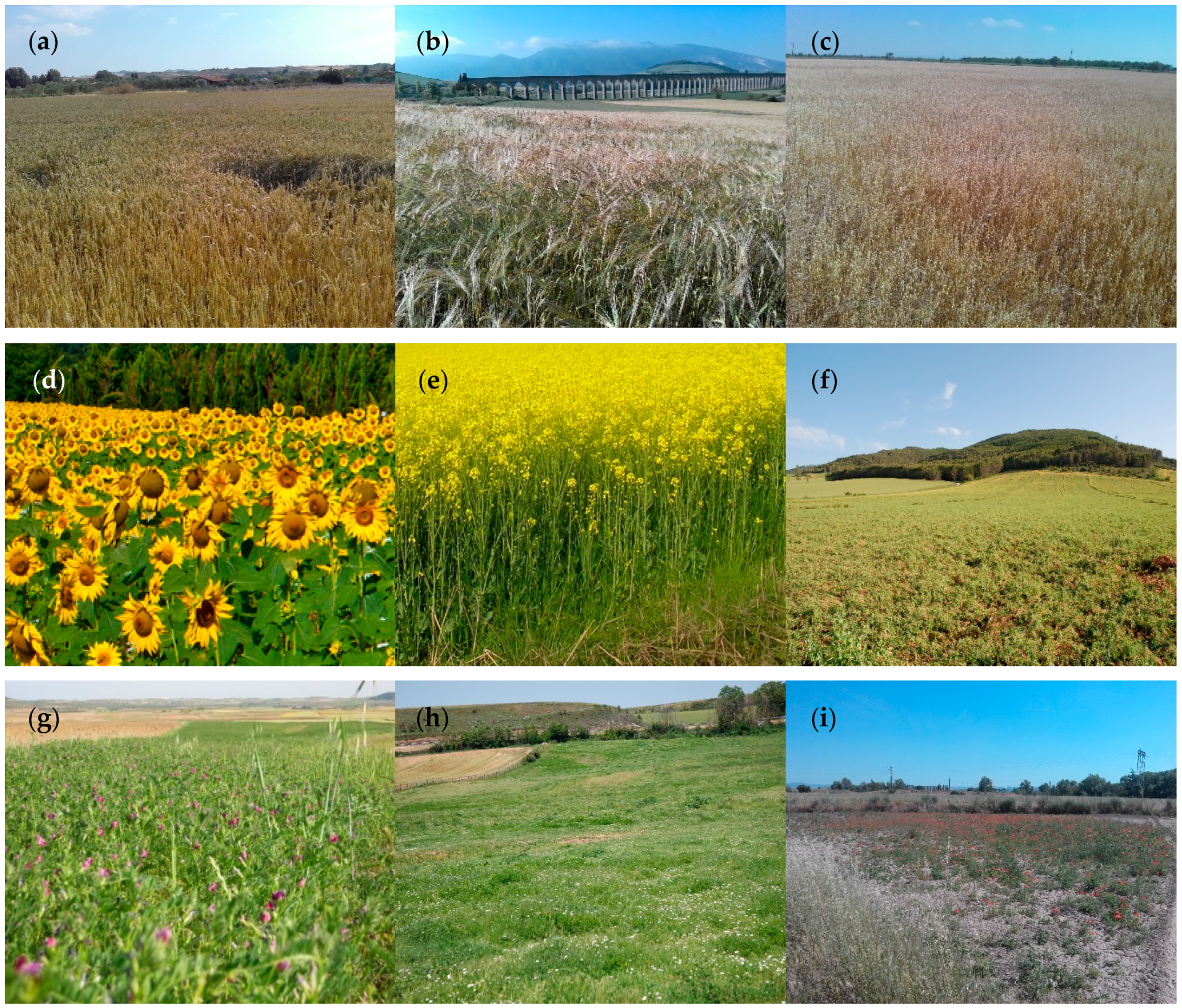
In this region, an area of 25 km × 25 km was selected, where rain-fed agriculture is the main land use. In particular, winter cereals are the most frequent crops. In the year studied, wheat represented 55% of the total cultivated area, whereas barley and oats accounted for 16% and 15%, respectively. Other crop types, found in much lower abundance, were sunflower, rapeseed, peas, vetch, permanent grasslands, and fallow. Photographs of the crops studied are given in Figure 2.

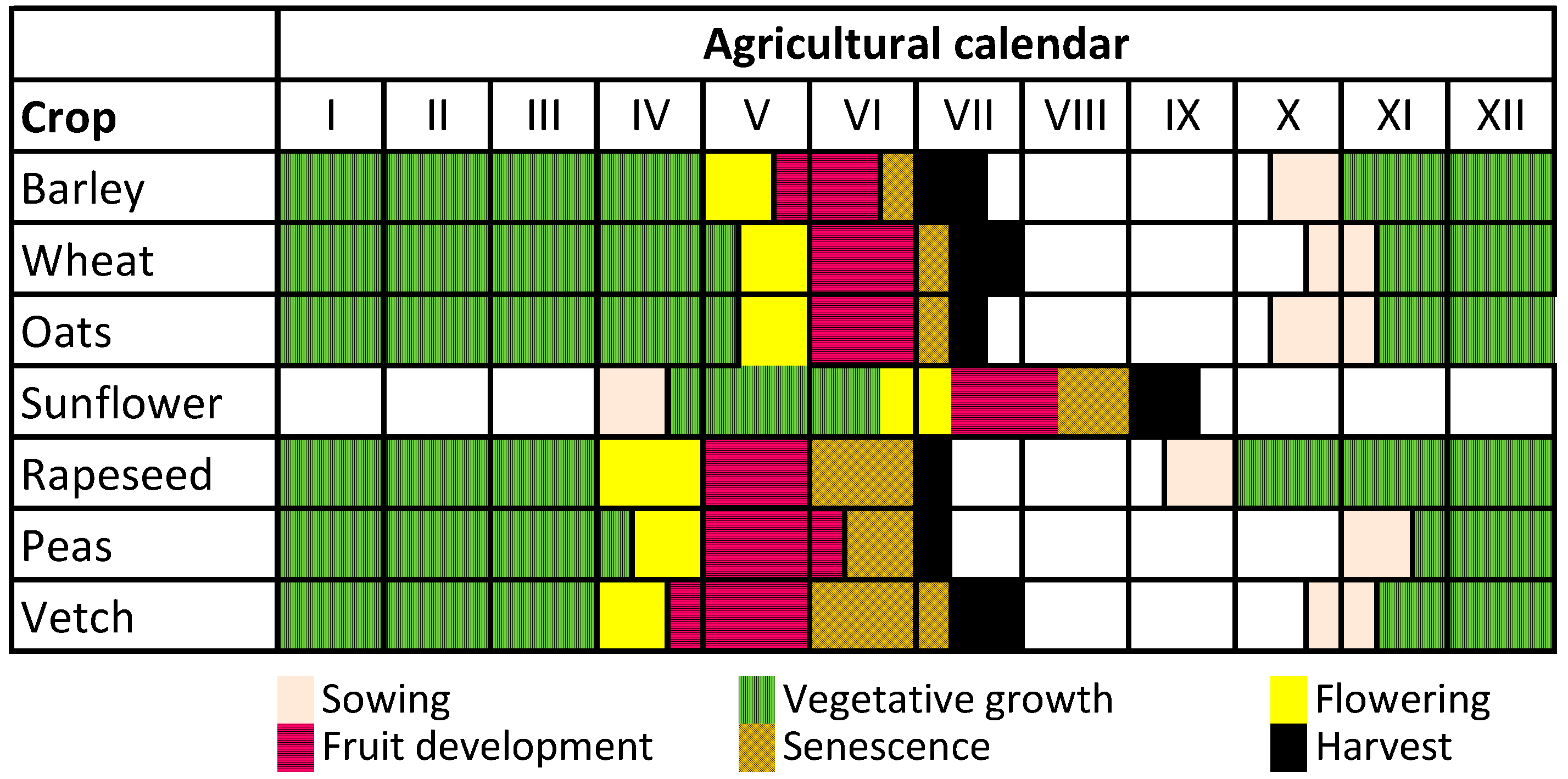
The agricultural calendar in this area is typical of rain-fed winter crops. Crops are normally sown in October and harvested in the beginning of July (Figure 3), with the exception of sunflower (planted in April and harvested in September). Although phenological stages develop very similarly in the three cereal crops (barley, wheat, and oats), barley plants flower and mature earlier. Barley stems are weaker than those of wheat and, as a result, after heading barley plants normally bend and their ears are inclined. On the contrary, wheat plants remain erected with vertical ears until harvest. Oat’s phenological events mimic wheat, but its inflorescences are different (i.e., panicles instead of ears). Rapeseed is sown earlier (in September) and flowers in April. In its vegetative phase rapeseed grows vigorously and develops a dense, bush-like canopy that can reach a height of 1–1.5 m. During May rapeseed fruits (pods) develop and then start to ripen. Afterwards, senescence starts and ends at the end of June when plants die and pods are completely dry and hard. Peas and vetch are legume crops grown as forage in this area. Their calendar is also typical of winter crops, although their sowing date is usually later (end of October or November). They are shorter than cereal plants and their canopies have a dense random structure. After flowering they develop pods that ripen and get dry and hard. Pea pods are longer and thicker than vetch’s. Sunflower is the most different crop in terms of calendar and canopy configuration. Sunflower is a broadleaved plant with thick and long stems (compared to the other crops of this study), which is planted in April. Plants usually have a separation of 20–30 cm between each other and after a short and quick vegetative phase they develop large circular flowers that fill in with seeds. Flowers dry and senescence occurs during summer; the crop is finally harvested in September.

Grasslands in this area are mostly permanent covers with no sowing and harvest dates. Instead they are cut (some of them grazed) several times during the season (normally three times), and experience different phenological events depending on their species composition. This cover is therefore very heterogeneous and diverse in terms of management. Finally, fallow fields are normally present for a one-year duration in a rotation cycle of approximately five years. Fallow fields are also quite heterogeneous depending on the techniques used for weed management (e.g., mechanical, chemical, etc.).

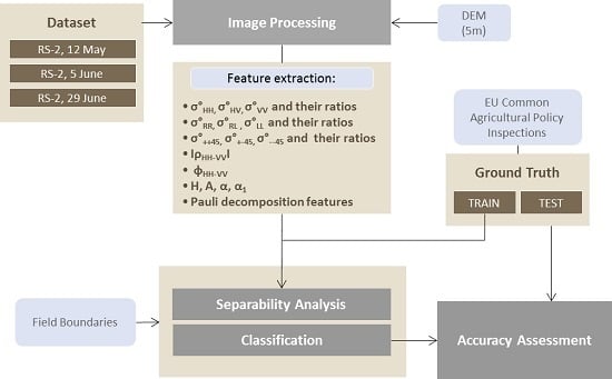
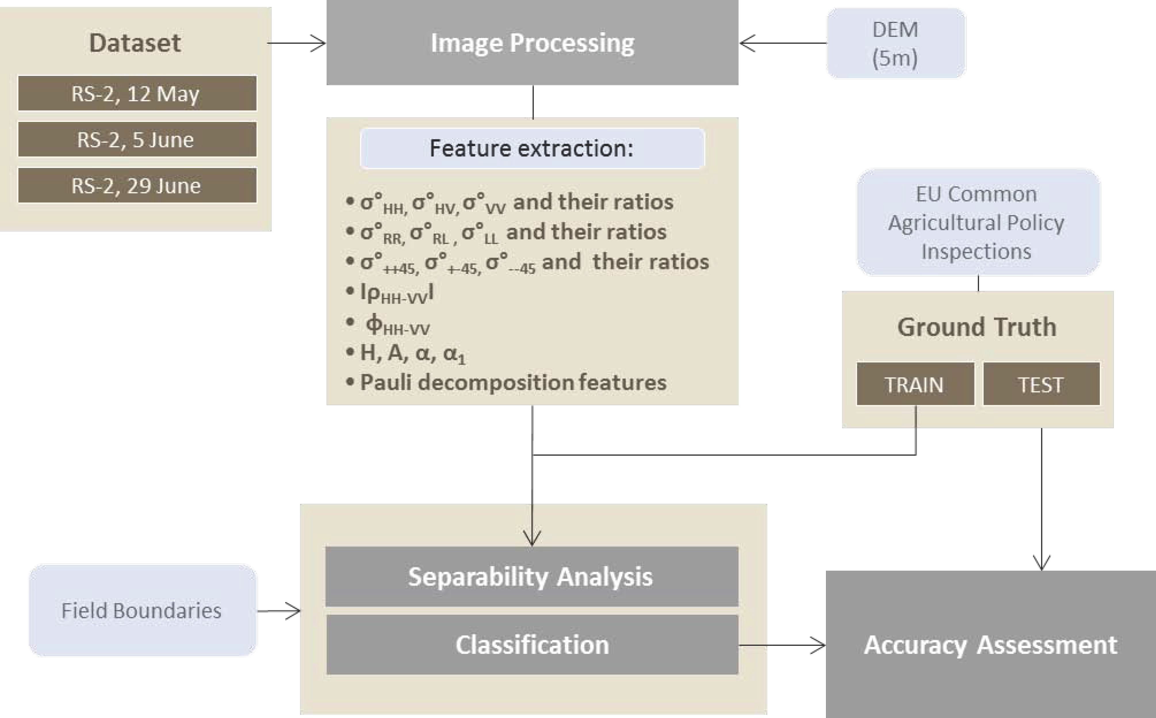
During the year 2010, a series of RADARSAT-2 scenes were acquired over the area. Based on a previous analysis [30], the following three acquisition dates were selected: 12 May, 5 June, and 29 June, since they represented optimal dates for accurate crop separation and classification, and in fact, including earlier acquisition dates did not result in higher accuracies [30]. All scenes were acquired in Fine Quad-Pol mode and as Single-Look-Complex products with a spatial resolution of 5.4 m in range and 8.0 m in azimuth. In all cases, the average incidence angle was around 30°.

The ancillary data used consisted of a digital elevation model (DEM) of 5 m, a vector file with field boundaries, and ground truth data resulting from the inspections of the EU CAP program (information not publicly available). The EU CAP program provides subsidies to European farmers depending on the crops being cultivated on each field and the management techniques used. Local administrations are required to inspect a sample of these CAP declarations, so as to verify that farmer declarations conform to reality (i.e., the crops declared by farmers are actually grown on each field). In this particular case, the Government of Navarre inspected a 5% sample of fields selected at random. The total area of the fields inspected within the studied area was above 1600 ha. With this information, a database of 928 fields with known crop class was generated. The number of fields per class varied proportionally to the area covered by each crop in the region. Accordingly, the database had the following number of fields per class: Wheat, 476; Barley, 168; Oats, 165; Sunflower, 24; Rapeseed, 10; Peas, 8; Vetch, 26; Grassland, 17; and Fallow, 34. One portion (2/3) of this information was used as ground truth to build the crop signatures (622 fields), and the rest for accuracy assessment (306 fields); both sets were obtained at random, keeping the same training/test proportions for each class. It should also be taken into account that field size varied strongly with average field size being the largest for fields corresponding to sunflower and rapeseed (>3 ha), followed by grasslands (~2 ha), cereals and fallow (1–2 ha), and lastly peas and vetch (<1 ha).

3. Methodology

Figure 4 shows the general work-flow of this study. In the following subsections different tasks are explained in detail.

3.1. Image Processing

Image processing consisted of the following steps: (1) slant range to ground range conversion; (2) orthorectification; (3) calibration; and (4) speckle filtering. Orthorectification was carried out using a rigorous sensor model that required no ground control points and provided location accuracies below 1 pixel. Image calibration was performed using local incidence angle values computed from the DEM available, to correct radiometric effects of topography. A 3 × 3 window Gamma-MAP filter was used for speckle reduction. This adaptive filter is effective for reducing speckle while preserving linear characteristics and discrete scatterers [32]. The resulting processed images were resampled to a pixel size of 5 m. Finally, field medians were computed excluding border pixels by applying a 1-pixel buffer to the field boundary vector file. Image processing was performed using Geomatica 10.3, NEST-5.1 and PolSARpro 5.0.

In addition, different polarimetric features were calculated. Backscattering coefficients (σ°) at different polarization bases were calculated using polarization synthesis. In particular, circular and 45° linear polarization bases were used. The first consists of right-handed and left-handed polarization states, leading to two co-polarized (RR and LL) and two cross-polarized (RL and LR) channels. And the second consists of +45° and −45° polarization states, leading to two co-polarized (++,−−) and two cross-polarized (+−,−+) polarization channels. As already explained, for each polarization basis only one cross-polarized channel was used since agricultural fields can be assumed to be reciprocal targets and provide the same information in both cross-polarized channels. Next, backscatter ratios were calculated for the three polarization bases. The polarimetric features considered were, the magnitude (|ρ_HH-VV|) and phase (φ_HH-VV) of linear co-pol coherence, the Pauli decomposition components surface scattering (|S_HH + S_VV|), volume scattering (|S_HV|) and double-bounce (|S_HH − S_VV|) and the Cloude-Pottier decomposition components entropy (H), average alpha angle (α), dominant alpha angle (α₁) and anisotropy (A). Accurate estimation of H/A/alpha and co-pol coherence parameters requires spatial averaging, thus a 5 × 5 window was considered for alpha and co-pol coherence, and a 9 × 9 for H and A that are more affected by speckle noise [33]. This averaging limits the utility of these polarimetric features for small fields.

3.2. Separability Analysis

Separability or statistical dissimilarity is a measure of difference between two targets (e.g., agricultural crops) as observed on a particular channel or feature. Different separability measures exist and their underlying assumptions and interpretation differ. Backscatter coefficients and polarimetric features do not necessarily follow Gaussian probability distribution functions (pdfs). Therefore, separability measures not restricted to Gaussian pdfs need to be used to analyze SAR data. With this aim, the Jeffries–Matusita (JM) distance was used (Equation (1)), as it does not make previous assumptions about observations’ pdfs [34]. In this work, separability analysis consisted of the evaluation of the JM distance between pairs of crops for different features and dates.

$$J_{ij}=\left\{{{\displaystyle \int }}^{\text{}}{\left[\sqrt{p\left(x|{\omega }_i\right)}-\sqrt{p\left(x|{\omega }_j\right)}\right]}^{2}dx\right\}$$

(1)

where, J_ij is the JM distance between a pair of classes ω_i and ω_j, x refers to the observed feature (e.g., backscatter coefficient or polarimetric feature), and p(x|ω_i) and p(x|ω_j) are the conditional probability density functions for x given ω_i and ω_j, respectively.

The JM distance ranges from 0 to 2, with J_ij = 0 representing two classes that completely overlap, and J_ij = 2 two classes that are completely separable. Values below 1 represent poor separability, 1–1.5 corresponds to intermediate separability, and 1.5–2 corresponds to high separability [35].

3.3. Classification Algorithm

This study used the Random Forests (RF) classification algorithm [36] to classify different crop types based on RADARSAT-2 derived features. RF is a nonparametric supervised classification scheme with no a priori assumptions on the input data sets’ pdfs. RF is an ensemble learning technique that generates many decision trees that are aggregated to classify. Tree diversity is guaranteed because trees are trained using different subsets and use different split rules at their nodes. In particular, each tree within the ensemble is trained on a random subset of the original data, resampling the data with replacement. Then, tree nodes are split using the best split variable among a subset of randomly selected predictive variables. As a result, different classification results are obtained from each tree, and a simple majority vote is used to create the final classification result. The RF technique has been applied to a wide variety of disciplines, and in the last decade it has been used with success in remote sensing applications including SAR classification studies [14,37,38].

In this work different RF classifications were performed using the package “randomForest” run on the free software for statistical computing R. The number of trees (“ntree”) was optimized and set to 200. The number of input variables considered for the random selection of the best splitting variable at each node (“mtry”) was taken as the square root of the total number of input variables considered for each classification. Similar to most classifiers, RF produces weak results when learning from heavily imbalanced training datasets, favoring the majority classes and resulting in a poor prediction of the minority classes [38]. To avoid this behavior different strategies can be followed, such as down-sampling the majority classes or over-sampling the minority classes so that they obtain the same training sample size as the majority ones [39]. In this work the latter option was implemented, but as in [40], rather than simply replicating the minority training sites, synthetically generated training sets were created by randomly perturbing each training site at around one standard deviation of the feature space. This way synthetic training sets statistically equal to the original ones were obtained with a size equal to that of the most frequent class (i.e., wheat).

Different RF classification models were constructed using the same training set but different input features (described in Section 3.1). Results were compared with an independent test set to quantitatively assess classification performance. For this aim, standard accuracy assessment metrics were calculated, i.e., overall accuracy (OA), Kappa coefficient, producer’s (PA), and user’s accuracies (UA).

4. Results

4.1. Descriptive Analysis

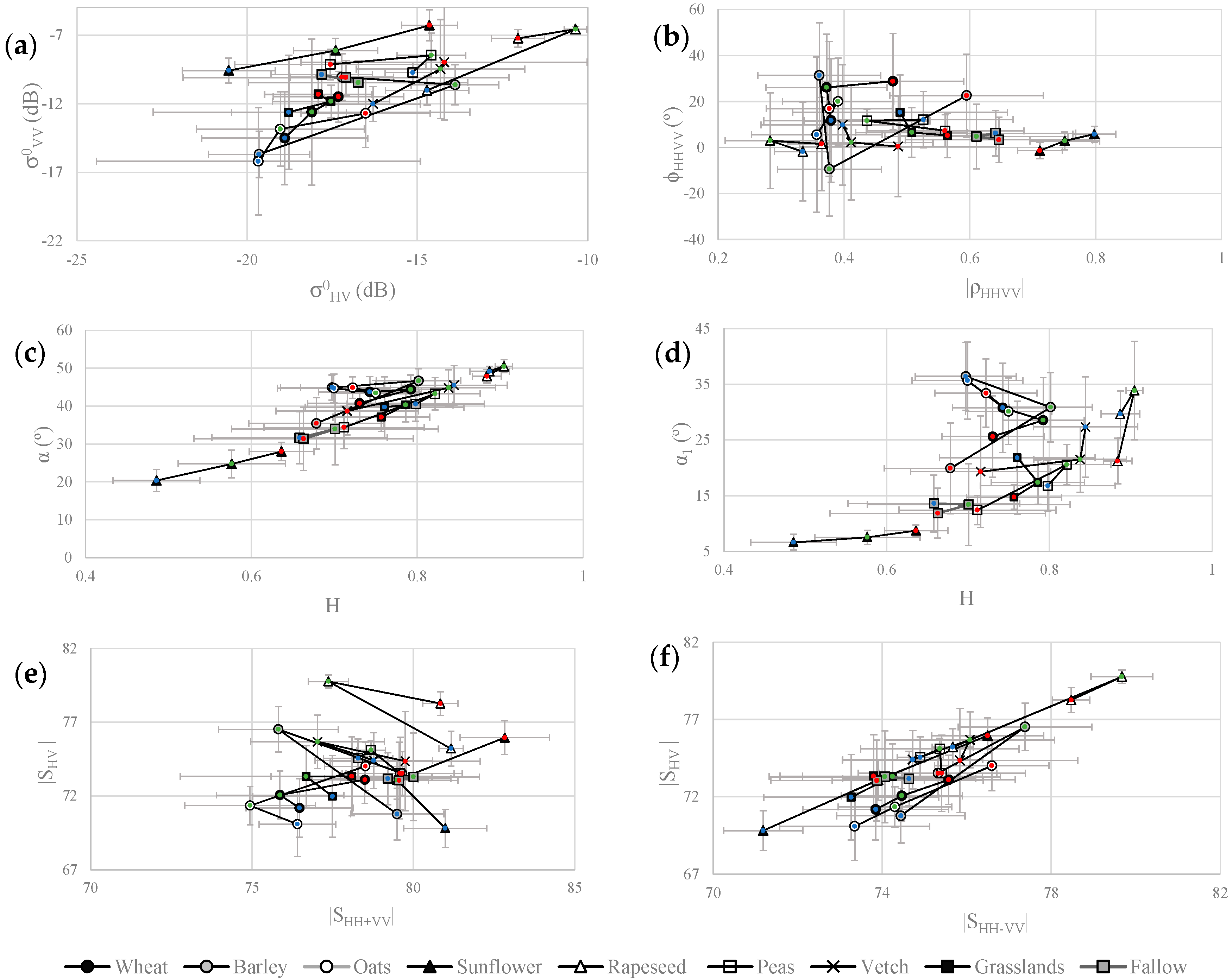
As a preliminary step to the separability analysis and classification, a descriptive analysis of crops’ behavior was made for the different features and dates. Figure 5 shows scatterplots of the most significant results that were obtained.

Rapeseed produced a significant volume scattering contribution and this can be clearly seen in its high σ°_HV value, its alpha value around 45°, and its high |S_HV| component, especially for the 5 June scene; similar results for rapeseed were obtained in [41]. The heterogeneous structure of the rapeseed canopy caused a strong depolarization of waves and for this reason the value of H was the highest and the |ρ_HH-VV| the lowest.

Due to the late sowing date of sunflower, at the time of image acquisition this crop was in its vegetative phase, with rather small plants (20–50 cm high) that did not completely cover the soil. As a result, its main scattering mechanism was surface scattering, illustrated by a high |ρ_HH-VV| and a φ_HH-VV close to 0° with a very low dispersion (much lower than that of the other crops). This was also confirmed by the lowest values of H and alpha angle, identifying surface scattering as the dominant mechanism. As sunflower plants grew, |ρ_HH-VV| decreased and H increased, illustrating a transition to other scattering mechanisms (volume and double bounce).

Generally, dominant alpha (α₁) took lower values than the average alpha (α) but both angles were quite similar if different crops were compared. Sunflower and fallow fields took the lowest values (i.e., surface scattering) and rapeseed and oats the highest, with values close to 45° (i.e., volume scattering).

H values were quite high for all crops except for sunflower (as mentioned above), with values above 0.7 for most crops and dates. After rapeseed (already discussed), peas and vetch had the highest H values; these are crops with a short, bush-like canopy structure. Cereals had slightly lower H values, although barley had a distinctive peak in H on 5 June, likely corresponding to barley ears filling. As ears fill in, barley plants lose their vertical structure and bend at random angles before the plants ripen, which actually takes place earlier than in other cereal crops. This effect is also visible in other polarimetric features. For instance, |ρ_HH-VV| had quite a high value in barley for the 29 June scene, probably indicating that harvesting had already taken place. Again, this was confirmed by the decrease in H and alpha angle.

For most of the crops, the increase of Pauli surface scattering (|S_HH+VV|) on 29 June was clearly apparent. At this time, most winter crops were senescent or even harvested, so electromagnetic radiation could penetrate further in the canopies, leading to an increased surface contribution.

Overall, rapeseed and sunflower were the crops with the largest dynamic range over the time period studied. In contrast, grasslands and fallow remained mostly constant for any of the features studied without showing any clear pattern. These classes showed a very high variability (see error bars in Figure 5), which could probably be a consequence of great differences in management (grassland cutting and weed control in fallow lands) and phenology of these covers.

4.2. Separability Analysis

JM distance was computed to evaluate the separability between each pair of crops for each feature and date. Then, average distance values for each crop with the rest were computed for each date, as well as the average separability of all crop pairs for each feature. It can be observed that JM distance values obtained have a clear temporal variability (

Table 1. Average JM distance for each crop and date, as well as the average of all crop pairs, for σ°_HH, σ°_HV, σ°_VV, and their ratios. Colors represent values above 1.00 (blue) and above 1.50 (green), and shades represent the different dates evaluated.

	Wheat	Barley	Oats	Sunflower	Rapeseed	Peas	Vetch	Grassland	Fallow	Average
σ°HH	0.24	0.20	0.33	0.25	0.58	0.35	0.22	0.46	0.36	0.33
	0.52	0.59	0.50	0.66	1.57	0.52	0.39	0.62	0.41	0.64
	0.31	0.34	0.30	0.92	0.85	0.36	0.40	0.77	0.55	0.53
σ°HV	0.49	0.66	0.59	0.87	1.16	1.23	0.70	0.51	0.50	0.75
	0.73	1.01	0.91	0.81	1.90	1.03	0.67	0.62	0.56	0.92
	0.47	0.53	0.43	1.00	1.59	0.44	0.45	0.50	0.42	0.65
σ°VV	0.84	1.16	1.07	1.03	0.86	1.07	0.78	0.61	0.79	0.91
	0.83	0.68	1.11	1.12	1.75	0.80	0.56	0.82	0.62	0.92
	0.64	0.46	0.89	1.27	1.26	0.58	0.43	0.63	0.59	0.75
σ°HH /σ°VV	0.72	1.11	0.92	1.36	0.76	0.76	0.57	0.53	0.58	0.81
	0.58	0.69	0.77	0.83	0.96	0.91	0.45	0.46	0.49	0.68
	0.72	0.60	1.08	0.72	0.69	0.54	0.63	0.54	0.56	0.68
σ°HV /σ°HH	0.40	0.66	0.41	0.95	1.01	0.89	0.48	0.46	0.45	0.63
	0.44	0.48	0.55	1.01	1.42	0.75	0.38	0.41	0.39	0.65
	0.34	0.42	0.32	0.65	1.55	0.42	0.34	0.74	0.31	0.57
σ°VH /σ°VV	0.47	0.54	0.57	1.76	0.85	0.83	0.45	0.48	0.82	0.75
	0.41	0.75	0.43	1.47	1.12	0.82	0.48	0.49	0.50	0.72
	0.37	0.35	0.69	0.99	0.95	0.55	0.37	0.75	0.41	0.60

12 May

5 June

29 June

,

Table 2. Average JM distance for each studied crop and date as well as the average of all crop pairs, for σ°_RR, σ°_RL, σ°_LL, and their ratios. Colors and shades as in Table 1.

	Wheat	Barley	Oats	Sunflower	Rapeseed	Peas	Vetch	Grassland	Fallow	Average
σ°RR	0.37	0.51	0.46	0.91	1.01	0.88	0.59	0.55	0.39	0.63
	0.55	0.89	0.65	0.74	1.82	0.93	0.48	0.56	0.50	0.79
	0.38	0.45	0.43	0.83	1.65	0.39	0.43	0.63	0.51	0.63
σ°RL	0.58	0.80	0.81	1.07	0.75	0.80	0.46	0.51	0.66	0.72
	0.76	0.67	0.92	1.12	1.47	0.57	0.52	0.76	0.53	0.81
	0.50	0.44	0.56	1.56	1.07	0.62	0.52	0.76	0.58	0.73
σ°LL	0.39	0.51	0.45	0.92	1.10	0.99	0.61	0.58	0.51	0.67
	0.55	0.95	0.64	0.69	1.85	0.92	0.58	0.65	0.61	0.83
	0.41	0.49	0.47	0.89	1.50	0.37	0.49	0.77	0.59	0.67
σ°RR/σ°LL	0.18	0.20	0.20	0.25	0.33	0.35	0.31	0.16	0.19	0.24
	0.17	0.18	0.21	0.39	0.59	0.18	0.45	0.16	0.25	0.29
	0.17	0.17	0.14	0.47	0.28	0.22	0.39	0.14	0.16	0.24
σ°RL /σ°RR	0.46	0.60	0.47	1.72	1.06	0.72	0.46	0.47	0.82	0.75
	0.39	0.53	0.39	1.48	1.03	0.63	0.39	0.46	0.49	0.64
	0.40	0.35	0.61	1.04	1.21	0.40	0.48	0.46	0.42	0.60
σ°RL /σ°LL	0.47	0.55	0.53	1.74	0.95	0.77	0.47	0.48	0.95	0.77
	0.41	0.55	0.40	1.47	1.09	0.57	0.49	0.47	0.56	0.67
	0.37	0.40	0.61	1.15	1.09	0.36	0.46	0.74	0.47	0.63

12 May

5 June

29 June

,

Table 3. Average JM distance for each studied crop and date as well as the average of all crop pairs, for σ°₊₊, σ°₊₋, σ°₋₋, and their ratios. Colors and shades as in Table 1.

	Wheat	Barley	Oats	Sunflower	Rapeseed	Peas	Vetch	Grassland	Fallow	Average
σ°++	0.56	0.74	0.73	0.63	0.54	0.54	0.45	0.49	0.51	0.58
	0.81	0.56	0.90	0.92	1.46	0.49	0.57	0.78	0.64	0.79
	0.53	0.46	0.52	1.38	1.16	0.62	0.52	0.73	0.57	0.72
σ°R+-	0.31	0.46	0.33	0.94	1.06	0.49	0.54	0.55	0.38	0.56
	0.48	0.81	0.56	0.74	1.81	0.79	0.58	0.67	0.60	0.78
	0.35	0.39	0.39	0.65	1.45	0.43	0.47	0.76	0.63	0.61
σ°--	0.49	0.77	0.73	0.91	0.64	0.58	0.34	0.47	0.52	0.61
	0.79	0.58	0.97	0.96	1.57	0.75	0.50	0.72	0.51	0.82
	0.56	0.50	0.57	1.43	1.30	0.67	0.47	0.86	0.51	0.76
σ°++/σ°--	0.22	0.24	0.22	0.59	0.36	0.46	0.42	0.22	0.24	0.33
	0.17	0.23	0.19	0.70	0.17	0.19	0.28	0.40	0.16	0.28
	0.23	0.19	0.35	0.58	0.28	0.40	0.38	0.41	0.20	0.33
σ°+- /σ°++	0.55	0.70	0.63	1.60	1.05	1.06	0.51	0.49	0.77	0.82
	0.47	0.38	0.53	1.47	0.65	0.47	0.38	0.49	0.49	0.59
	0.47	0.36	0.66	1.24	0.92	0.56	0.35	0.45	0.54	0.62
σ°-+ /σ°--	0.43	0.71	0.53	1.48	0.87	0.42	0.41	0.40	0.71	0.66
	0.48	0.39	0.51	1.48	0.87	0.45	0.38	0.54	0.51	0.62
	0.44	0.35	0.66	1.21	1.04	0.39	0.38	0.49	0.51	0.61

12 May

5 June

29 June

,

Table 4. Average JM distance for each studied crop and date as well as the average of all crop pairs, for the Cloude–Pottier features H-A-α and α₁. Colors and shades as in Table 1.

	Wheat	Barley	Oats	Sunflower	Rapeseed	Peas	Vetch	Grassland	Fallow	Average
α	0.56	0.62	0.58	1.81	1.21	0.63	0.56	0.57	0.98	0.83
	0.51	0.61	0.56	1.74	1.22	0.50	0.48	0.62	0.76	0.78
	0.55	0.45	0.94	1.26	1.34	0.52	0.44	0.64	0.58	0.75
A	0.20	0.17	0.17	0.22	0.60	0.15	0.34	0.32	0.17	0.26
	0.23	0.16	0.25	0.40	0.52	0.15	0.23	0.25	0.14	0.26
	0.19	0.19	0.18	0.42	0.28	0.30	0.26	0.19	0.14	0.24
H	0.59	0.68	0.63	1.68	1.38	0.56	0.79	0.48	0.61	0.82
	0.53	0.52	0.62	1.54	1.58	0.54	0.58	0.50	0.65	0.78
	0.39	0.36	0.38	0.80	1.63	0.32	0.31	0.48	0.43	0.57
α1	0.60	0.89	0.81	1.69	0.83	1.00	0.53	0.54	1.06	0.88
	0.56	0.73	0.71	1.73	0.76	0.75	0.53	0.83	0.79	0.82
	0.75	0.55	1.27	1.46	0.83	0.88	0.57	0.94	0.74	0.89

12 May

5 June

29 June

and

Table 5. Average JM distance for each studied crop and date as well as the average of all crop pairs, for Pauli decomposition features (|S_HH − S_VV|, |S_HV|, and |S_HH + S_VV|), |ρ_HH-VV|, and φ_HH-VV. Colors and shades as in Table 1.

	Wheat	Barley	Oats	Sunflower	Rapeseed	Peas	Vetch	Grassland	Fallow	Average
|SHH − SVV|	0.52	0.54	0.68	0.88	0.86	1.02	0.40	0.52	0.72	0.68
	0.68	0.47	0.85	0.80	1.32	0.58	0.37	0.44	0.38	0.66
	0.36	0.24	0.46	0.99	0.86	0.25	0.25	0.38	0.24	0.45
|SHV|	0.40	0.50	0.54	0.83	0.89	0.69	0.52	0.32	0.39	0.56
	0.73	0.91	0.97	0.68	1.82	1.02	0.68	0.53	0.54	0.88
	0.42	0.41	0.34	0.68	1.39	0.29	0.32	0.30	0.32	0.50
|SHH + SVV|	0.32	0.33	0.36	1.20	0.92	0.73	0.34	0.37	0.34	0.55
	0.42	0.66	0.45	0.58	1.55	0.33	0.36	0.37	0.40	0.57
	0.29	0.34	0.36	0.36	1.30	0.26	0.30	0.45	0.42	0.45
|ρHH-VV|	0.49	0.53	0.52	1.70	0.86	0.51	0.44	0.45	0.85	0.71
	0.46	0.49	0.46	1.66	0.85	0.42	0.39	0.60	0.71	0.67
	0.41	0.42	0.71	1.27	1.02	0.37	0.37	0.58	0.50	0.63
φHH-VV	0.26	0.45	0.34	0.89	0.31	0.30	0.26	0.26	0.38	0.38
	0.49	0.46	0.38	0.80	0.29	0.67	0.33	0.31	0.27	0.44
	0.55	0.44	0.42	0.88	0.33	0.49	0.35	0.35	0.36	0.46

12 May

5 June

29 June

).

Average JM distances were low (<1.0) in most cases. This was somewhat expected, due to the averaging and the similarities existing between many of the crops studied, in terms of their agricultural calendar and morphology (see Section 2). However, sunflower and rapeseed showed a separability > 1.0 (and even >1.5 in some cases) with the rest for certain dates and features. Average JM distance values for cereals (i.e., wheat, barley, and oats) were normally low due to their mostly similar behavior during the growing season. In particular, wheat had a separability < 1 in all the linear backscatter coefficients and their ratios. Barley had three separability peaks above 1.0, one on 12 May in σ°_VV, a second one on 5 June in σ°_HV, and a third on 12 May in σ°_HH/σ°_VV. The first and third correspond to the moment where the flag leaf was deployed, whereas the second could be related to the influence of barley ears. In turn, oats had a separability >1.0 in σ°_VV on the first two dates and in σ°_HH/σ°_VV on the last (Table 1). This results were mostly in coincidence with [35].

The average JM distance of peas was quite good (>1.0) for σ°_HV and σ°_VV, obtaining better results on 12 May and 5 June, corresponding with the phase of fruit (pod) development. In general, backscatter ratios did not result in significantly higher separability values than backscatter coefficients. Grasslands, fallow, and vetch were the crops with the lowest separabilities in all the features and dates studied.

Different polarization bases did not appear to provide significant improvements in the outcome of separability (Table 2 and Table 3). In general, sunflower and rapeseed had high JM distances (>1.0 and even >1.5 in some cases) with other crops in circular and +45°−45° bases. On the contrary, for cereals, neither cases obtained higher separabilities than those obtained with linear (H-V) basis. As in the previous case, backscatter ratios did not seem to provide enhanced separabilities, with the exception of sunflower, which was best separated on 12 May in both the circular and +45°−45° cross-pol ratios (1.74 and 1.60, respectively). Furthermore, a very low separation (<0.6) was observed for all crops in the circular and +45°−45° co-pol ratios.

JM distances obtained for H-A-α Cloude–Pottier decomposition parameters were variable (Table 4). The highest distance values were obtained by α₁, followed by α. Therefore, it seems that for this type of target (crops) α₁ is more informative than α. However, there were some exceptions, like sunflower, which showed the highest JM distances with α, although closely followed by H and α₁ on 12 May and 5 June. Also, H and α obtained the highest separabilities for rapeseed, particularly on 29 June. For cereals, JM distances were, in general, low because of their similar characteristics, already mentioned above. However, oats had quite a high JM distance for α₁ on 29 June (and slightly lower for α), this represented the highest separability for this crop in all the features studied. This is due to higher α₁ values for oats (~33°) compared to wheat (~26°) and barley (~20°) (see Figure 5) in the last part of the season, demonstrating that oats ripen slower and keep a certain volume scattering component, whereas wheat and barley move faster to a surface scattering behavior.

Peas and vetch showed low separability values with the only exception of α₁ on 12 May for peas (Table 4), coinciding with the phenological stage of pod development. It must be taken into account that peas and vetch had the smallest field sizes and this might seriously compromise the accuracy of these polarimetric features due to the spatial averaging required for their calculation. On the contrary, the larger field sizes of sunflower and rapeseed might also favor the ability of H and α to separate them. Finally, anisotropy yielded very low separability distances for all crops, indicating no predominance of a second scattering mechanism (i.e., the second and third scattering mechanisms were at the same level).

Finally, Pauli decomposition parameters, co-pol coherence and phase difference were assessed (Table 5). In this case, and in agreement with the results showed above, sunflower and rapeseed yielded the highest distance values. Sunflower had its highest separabilities in |ρ_HH-VV|, particularly on 12 May and 5 June (1.70 and 1.66, respectively), whereas rapeseed was best separated in |S_HV| and |S_HH + S_VV| on 5 June and 29 June (1.55 and 1.30, respectively). For the other crops, |S_HV| and |S_HH − S_VV| (particularly on 5 June) resulted in the highest separabilities in this set of features. However, separabilities were not higher than those obtained with the backscatter coefficients and ratios with linear (H-V) basis.

4.3. Crop Classification

RF classification algorithm was used to evaluate the added value of quad-pol data by testing different polarization bases and polarimetric features in a multi-temporal crop classification scheme. Different classification models were built considering different inputs. First, model 0 consisted of VV-VH dual-pol configuration with just two backscattering coefficients in the two polarization channels. Then quad-pol configurations including three backscattering coefficients and their ratios were evaluated considering three polarization bases, i.e., linear H-V, circular and linear 45°, leading to models 1, 2, and 3, respectively (

Table 6. Classification accuracy measures using as input dual-pol vs. quad-pol with different polarization bases.

Model No		Quad-Pol			Overall Accuracy	Kappa
	Dual VV-VH	Linear H-V *	Circular †	Linear 45° ‡
0	x				0.79	0.69
1		x			0.79	0.69
2			x		0.66	0.53
3				x	0.70	0.57

* σ°_HH, σ°_HV, σ°_VV, and their ratios; ^† σ°_RR, σ°_RL, σ°_LL, and their ratios; ^‡ σ°₊₊, σ°₊₋, σ°₋₋, and their ratios.

).

The same results were obtained using either the dual-pol VV-VH (model 0) or the quad-pol configuration in linear H-V basis (model 1), providing OA and Kappa values of 0.79 and 0.69, respectively. However, quad-pol data in circular or 45° bases lead to lower accuracies (Table 6), particularly in the circular case.

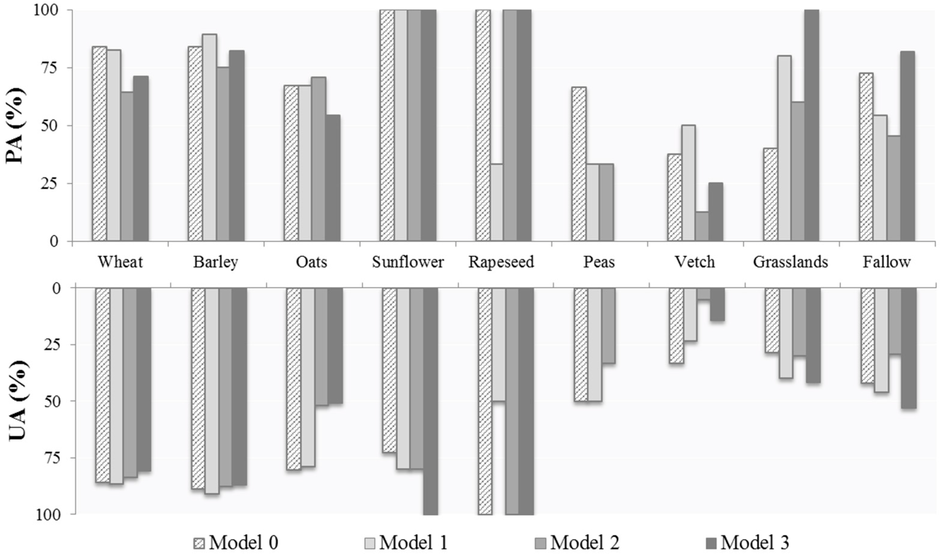
Figure 6 shows the accuracy obtained for individual crop classes on each model (0 to 3) representing the producer’s and user’s accuracy (%). PA represents the probability that a certain crop class on the ground is correctly classified, whereas UA refers to the probability that any field classified as a certain crop class in the image is actually this class on the ground. PA corresponds to errors of omission (fields of a certain class not classified as such) and UA to errors of commission (fields included erroneously in a certain class).

The best PA results were achieved for sunflower and rapeseed. Sunflower obtained a PA of 100% in the four modes tested, and so did rapeseed in models 0, 2, and 3. These results are in agreement with the high separability values obtained for these two classes, except for rapeseed in model 1, where a high proportion of fields were erroneously classified as peas. UA results for these two crops were slightly lower than PA values, and were highest for models 0, 2, and 3 for rapeseed and model 3 for sunflower. Wheat and barley yielded high accuracies for models 0 and 1, with PA and UA values above 75%. The third cereal crop, oats, had lower PA accuracies (mostly due to some oat fields being classified as wheat) with values around 70% for models 0, 1, and 2 and even lower for model 3. The UA values of oats were above 75% for models 0 and 1 but dropped down to 50% for models 2 and 3.

Minor crops (i.e., peas, vetch, and grasslands) had normally lower accuracies, since most classification models tested failed at classifying these crops. In particular, pea fields obtained the best results for model 0 with PA = 67% and UA = 50%; these values were lower for the other models tested. Vetch achieved even poorer results with a maximum PA of only 50% for model 1; circular and 45° bases resulted in even lower accuracies. The small field sizes of these two classes might be partly responsible of these poor results. Grasslands were also poorly classified with model 0 but its results improved clearly for model 1 and, especially for model 3, with PA values of 100%, although UA only reached 42%. This means that all grasslands test sites were classified as such, but several test fields of other classes (mostly wheat) were also incorrectly classified as grasslands. Finally, fallow fields had varying accuracies depending on the models tested. Overall, the high accuracies obtained with the VV-VH dual-pol configuration (model 0) and the quad-pol in 45° bases (model 3) seem very remarkable, with PA and UA values around 75% and 50%, respectively.

The inclusion of the different polarimetric features in the RF classification scheme improved classification accuracy measures in all cases (

Table 7. Classification accuracy measures when different polarimetric features were added to the H-V linear quad-pol data.

Model No	Feature Combination					Overall Accuracy	Kappa
	Linear H-V *	|ρHH-VV|, φHH-VV	Pauli	α, H, A	α1, H, A
4	x	x				0.84	0.76
5	x		x			0.81	0.72
6	x			x		0.82	0.73
7	x				x	0.82	0.73
8	x	x	x	x	x	0.86	0.79

* σ°_HH, σ°_HV, σ°_VV, and their ratios.

). In particular, the inclusion of coherence (|ρ_HH-VV|) and phase difference (φ_HH-VV) in model 4 outperformed the OA and Kappa values obtained with model 1 (with improvements of 0.05 in OA and 0.07 in Kappa). The other three models (models 5, 6, and 7) resulted in only minor accuracy enhancements. The best results were obtained when all the polarimetric features were used as input (model 8), with an OA of 0.86 and a Kappa value of 0.79. When compared to the VV-VH dual-pol configuration (model 0 in Table 6), these values represented improvements of 0.07 and 0.10 in terms of OA and Kappa, respectively.

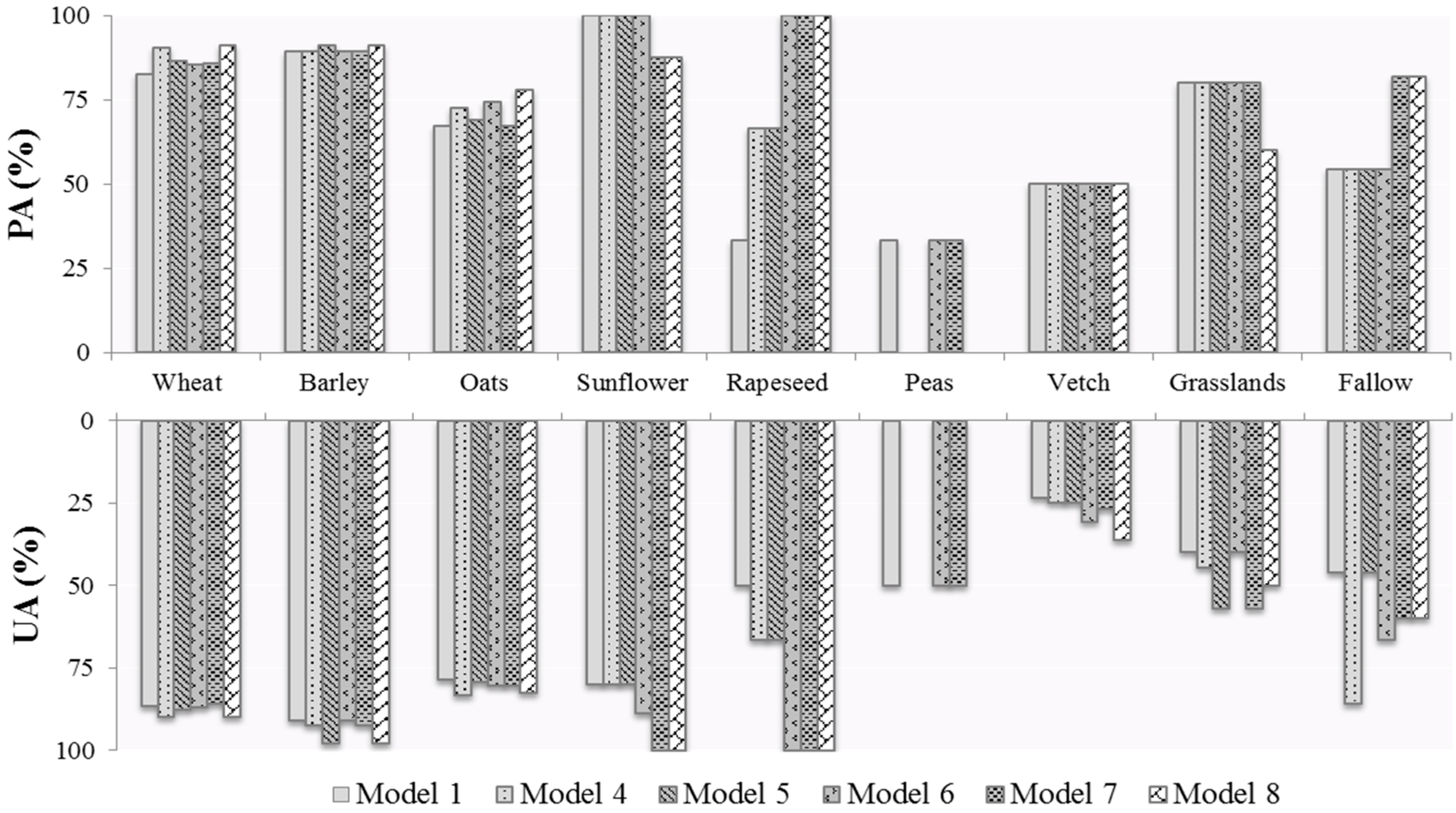
The results per crop (Figure 7) showed that polarimetric features contributed to slight improvements for wheat, barley, and oats; with PA and UA values increasing around 10% in the best cases. For wheat the addition of |ρ_HH-VV| and φ_HH-VV provided the best results, whereas for barley it was Pauli features and for oats |ρ_HH-VV| and φ_HH-VV and α/H/A. Sunflower obtained good results regardless of the polarimetric features added, with highest accuracies for model 6 (PA = 100% and UA = 89%). In turn, rapeseed clearly benefited from the addition of polarimetric features; with models 4 and 5 having PA and UA values around 65% and models 6, 7, and 8 topping 100%. The poorest results were obtained for peas, where none of the polarimetric features improved the accuracy values obtained for the VV-VH dual-pol case (Figure 6); models 1, 6, and 7 obtained the same results and models 4 and 8 were unable to correctly classify a single pea field (Figure 7). On the other hand, vetch yielded PA values of 50% for all cases regardless of the polarimetric features added; in this crop UA values were lower, with a maximum of 36% for model 8. Grasslands were quite successfully classified, with PA values of 80% for models 1–7; however, these values were exceeded when quad-pol data were transformed to 45° basis (model 3 in Figure 6). Similarly, fallow fields were reasonably identified in model 3 (Figure 6). This class achieved lower PA values for models 4–6 (Figure 7), whereas it increased again for models 7 and 8. 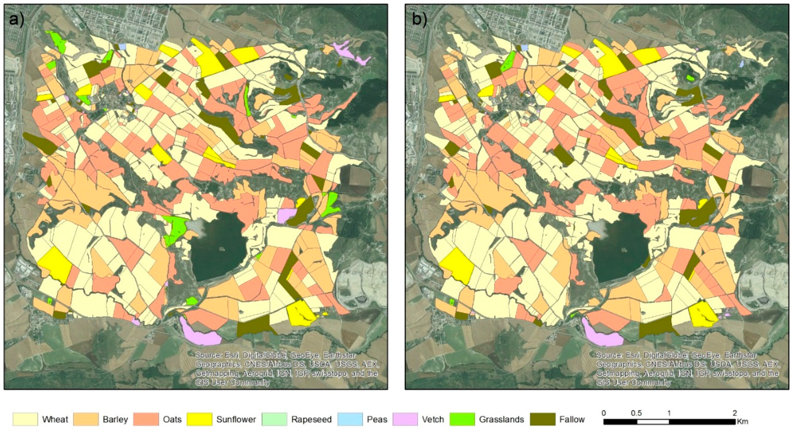This corresponds to the higher separability achieved by α₁ for this class (Table 4). These results are also visible in the classification maps provided in Figure 8, where the results of model 0 and model 8 are compared. It can be observed that their similarity is very high, with differences corresponding mainly to grasslands and minor crops like vetch and peas.

5. Discussion

The analyses performed (descriptive analysis, separability study, and classification) highlight the importance of linear backscatter coefficient values for crop classification. Using just three scenes acquired in key dates, a VV-VH dual-pol configuration was sufficient for accurately classifying most crops in the area (i.e., wheat, barley, oats, sunflower, and rapeseed). This result is remarkable and demonstrates the suitability of the Sentinel-1 nominal operational mode (dual-pol VV-VH) over land for agricultural applications. Although previous studies demonstrated the benefits of quad-pol data compared to single or dual-pol configurations for crop classification when just one acquisition date was available [22,42], when multi-temporal configurations were tested these differences were minor [8,43]. In fact, some studies [44,45] reported high classification accuracies with just three scenes acquired in key dates in dual-pol configurations, in coincidence with our results. Therefore, it seems that rather than a single-date quad-pol dataset, a multi-date dual-pol option provides enhanced crop classification accuracies.

However, results for minor crops (peas, vetch, grasslands, and, to a lesser extent, fallow) were not that successful and varied for the different models evaluated. It should be taken into account that the rather small size of fields of these classes (particularly peas and vetch) might have affected the accuracy of the calculation of some polarimetric features tested here, which required spatial averaging. On the other hand, the grasslands class can be very variable in terms of management practices; subdivision of this class into two or three classes according to their management would probably result in higher accuracies, but this could not be tested with our dataset. Similarly, fallow fields might also be difficult to identify because they can be very heterogeneous due to differences in weed management, previous crops cultivated, etc. Nonetheless, the classification based on V-H dual-pol data achieved an intermediate accuracy for peas, as did the quad-pol configuration for vetch. In turn, grasslands and fallow fields were accurately identified in some of the models tested, and these results are encouraging because of the heterogeneity of these classes in terms of management practices.

Overall, quad-pol data in different polarization bases (circular and 45° linear) showed worse results than those obtained with H-V linear basis. However, certain crops (i.e., grasslands and fallow) showed enhanced accuracies at 45° basis. Regarding the inclusion of different polarimetric features, co-pol coherence (|ρ_HH-VV|) and phase difference (φ_HH-VV), clearly improved the overall accuracy results obtained with quad-pol backscatter coefficients and ratios. Although, the other polarimetric features evaluated (Pauli and Cloude–Pottier decomposition features) showed some sensitivity to crop characteristics and good separabilities for some particular crops, their inclusion in the RF classifications did not result in clear improvements in the overall accuracy, probably because the information they provided was somehow redundant with that of the backscatter coefficients and ratios. Nonetheless, some improvements in the classification of some crops were observed after adding Pauli or Cloude–Pottier decomposition features. The inclusion of all the polarimetric features evaluated lead to overall classification performance metrics of OA = 0.86 and Kappa = 0.79; these values represented improvements of 0.07 and 0.10 in terms of OA and Kappa, respectively, when compared to the VV-VH dual-pol configuration.

All in all, this approach is almost ready to be used to operationally classify agricultural areas and, for instance, to reduce the number of fields inspected for the EU CAP program by local administrations. The accuracies obtained here suggest the operational readiness of this technique, at least for identifying major crops. Further improvements need to be done to successfully classify minor crops with small field sizes and heterogeneous classes like grasslands and fallow fields.

6. Conclusions

The results of this study demonstrate that C-band SAR data can be effectively used for crop classification. Major crops in the area achieved high classification accuracies, and in particular cereal crops (wheat, barley, and oats) could be adequately identified, which is remarkable due to their similarities in terms of morphology and agricultural calendar. It was observed that the use of different polarimetric bases (circular and 45° linear) did not produce clear benefits in terms of overall classification accuracy, although improvements were reported in the identification of some particular crops (i.e., grasslands and fallow). Regarding the addition of polarimetric features, co-pol coherence and phase difference clearly enhanced classification results, but Pauli and Cloude–Pottier decomposition features did not provide additional improvements. The classification using all the polarimetric features evaluated led to an overall accuracy of 0.86 and a Kappa value of 0.79; these values represented improvements of 0.07 and 0.10, respectively, when compared to the VV-VH dual-pol configuration. Hence, a VV-VH dual-pol configuration was still considered sufficient for accurately classifying major crops in the area as long as acquisitions in at least three key dates of the agricultural calendar were available. However, the method still needs to be adjusted to improve the classification of some crops that had small field sizes in this study (i.e., peas and vetch), heterogeneous cover (i.e., fallow and grasslands), and crops that are common in other parts of the world (e.g., corn, potato, or sugar beet). Today, Sentinel-1 data provide opportunities to make this application fully operational.