Development of a Class-Based Multiple Endmember Spectral Mixture Analysis (C-MESMA) Approach for Analyzing Urban Environments

Abstract

Multiple endmember spectral mixture analysis (MESMA) has been widely applied for estimating fractional land covers from remote sensing imagery. MESMA has proven effective in addressing inter-class and intra-class endmember variability by allowing pixel-specific endmember combinations. This method, however, assumes that each land cover type has an equal probability of being included in the model, and the one with the least estimation error (e.g., root mean square error) was chosen as the “best-fit” model. Such an approach may mistakenly include a land cover class in the model and overestimate its abundance, or it might omit a class from the model and subsequently lead to underestimation. To address this problem, this paper developed a land cover class-based multiple endmember spectral mixture analysis (C-MESMA) method. In particular, a support vector machine (SVM) method with reflectance spectra and spectral indices, including the normalized difference vegetation index (NDVI), the biophysical composition index (BCI), and the ratio normalized difference soil index (RNDSI), were employed to classify the image into six land cover classes: pure impervious surface area (ISA), pure vegetation, pure soil, ISA-vegetation, vegetation-soil, and vegetation-ISA-soil. With the information of land cover classes, an individual MESMA method was applied to each mixed class. Finally, the fractional maps were derived through integrating land cover fractions of each land cover class. Quantitative analysis of the resulting percent ISA (%ISA) and comparative analyses with traditional MESMA indicate that C-MESMA improved the estimation accuracy of %ISA.

1. Introduction

Spectral mixture analysis (SMA) has been widely applied to address the mixed pixel problem, a typical issue associated with medium- and coarse-resolution remote sensing imagery [1,2,3,4]. SMA assumes that each image pixel is comprised of several land cover classes, each of which has distinctive spectral signatures [1,5]. Traditional SMA approaches, with a fixed set of endmembers, perform reasonably well in areas with relatively homogenous land covers, particularly due to the easiness of identifying representative endmembers. In urban and suburban environments, however, inter-class and intra-class spectral variability widely exist [6,7,8,9,10]. Therefore, the capability of traditional SMA models in dealing with complex urban and suburban landscapes has been questioned, as the few endmembers may not be able to represent their corresponding land cover classes [11,12,13].

As an improved version of SMA, multiple endmember spectral mixture analysis (MESMA) developed by Roberts et al. [14] has successfully addressed the issues of endmember variability, and been widely applied to numerous fields, including impervious surface area (ISA) extraction, vegetation detection, and water management, etc. With MESMA, modeling errors, such as root mean square of the residual error (RMSRE) [15], have been typically considered as important criteria for selecting the best-fit model [14]. Generally, with the same number of endmembers, a model with a smaller RMSRE is chosen due to higher modeling accuracy. In the case of the availability of different endmembers’ numbers, the model with the fewer number of endmembers is selected when their RMSRE difference is trivial [11]. For successful spectral unmixing, the selection of an appropriate endmember set is essential, and the selection may greatly impact the performances [16]. In particular, if an endmember is mistakenly included in an SMA model, its abundance is likely to be over-estimated (e.g., greater than zero) [17]. Moreover, with the minimization of RMSRE as the criterion, some erroneously selected endmembers may have a better fit due to the existence of within-class and between-class spectral variability. As an example, spectral signatures of ISAs are similar to those of dry soils [18,19], and they are often mistakenly considered as endmembers in farmlands [20], where major land covers should only include vegetation and soil. This is primarily due to the selection of the ISA-vegetation model instead of the vegetation-soil model if only RMSRE are considered. As a result, the abundance of ISAs in farmlands is mistakenly over-estimated, while that of soil is underestimated by MESMA.

Recently, several approaches have been proposed to address the abovementioned deficiency. Franke et al. [21] proposed a hierarchical multiple endmember spectral mixture analysis to divide an image into several land cover types (several levels) to limit the spatial distribution of endmembers. Subclasses’ fractions were extracted from the upper level classification results. They found that the distribution of endmembers could be well constrained from the results obtained from the upper level, thereby improving the classification accuracy. Liu and Yang [22] introduced a similar method that classified the study area into rural and urban subsets with the assistance of road network density. MESMA was then carefully applied to urban subsets using three types of endmembers (vegetation, ISA, and soil), while a supervised classification model was employed for the rural area. Results illustrated that this method could minimize the spectral confusion between some urban land cover classes and agricultural landscapes.

Although these two methods can spatially constrain the distribution of endmembers, they cannot fully address the mix-pixel problem. A critical limitation of hierarchical MESMA [21] is that a pixel at level 1 is assigned to the ISA or the pervious surface class based on their corresponding fraction values resulted from a linear SMA. For instance, at level 1, a pixel is assigned to the impervious class with the ISA fraction higher than 50%, otherwise it is assigned to the pervious class. In other words, mixed pixels still exist in both pervious surface and ISA classes. Results from hierarchical MESMA is promising. However, these outcomes were only from the high spatial resolution image (four meters). This method still needs to be verified in the middle and coarse resolution images. In Liu and Yang’s research [22], a vegetation cover threshold was utilized to separate vegetation and non-vegetation. This threshold, however, is pixel-based, which would also contain mixed pixels in both vegetation and non-vegetation classes.

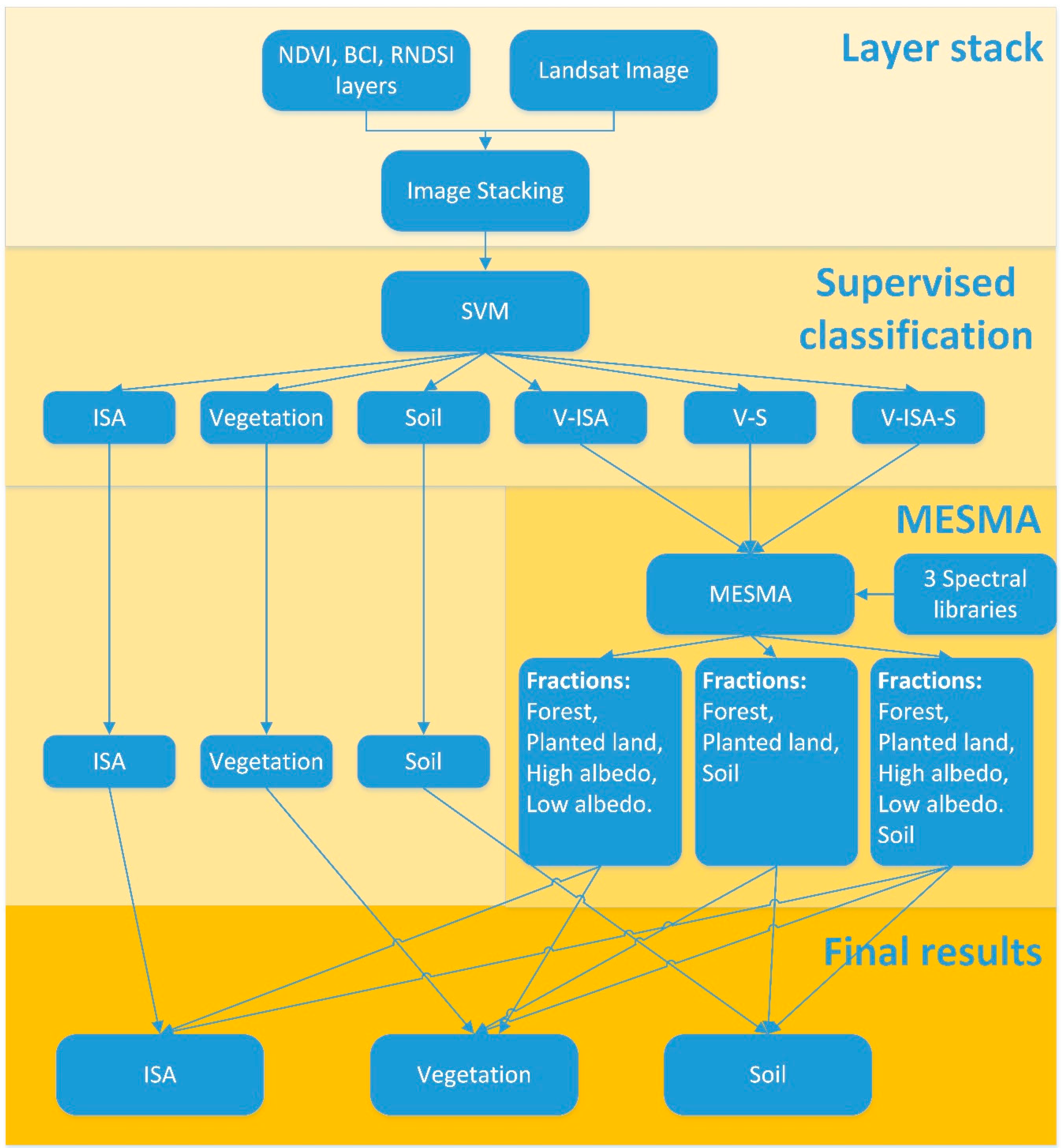
To address the aforementioned problems, this paper proposed a land cover class-based MESMA (C-MESMA) to map the land cover fractions of urban/suburban environments using a Landsat image. We developed this method through combining supervised classification and MESMA techniques. At the first level, a support vector machine (SVM) was applied to classify the study area into six land cover classes, three pure land cover classes (e.g., ISA, vegetation, soil) and three mixed land cover classes (e.g., ISA-vegetation, vegetation-soil, and vegetation-ISA-soil). For pure land cover classes, a fraction value of one is assigned to the corresponding class. For mixed land cover classes, a MESMA was implemented with corresponding spectral libraries to extract each endmember’s fractional coverage. Finally, fractions of ISA, vegetation, and soil of each land cover class were merged together to produce final fractional maps of ISA, vegetation, and soil. We tested the performance of the developed C-MESMA by comparing it to the results of the standard MESMA.

The next section introduces the study area and data sources. Section 3 presents the method of C-MESMA, as well as comparative analyses with traditional MESMA. Results of C-MESMA and an accuracy assessment are reported in Section 4. Finally, discussion and conclusions are provided in Section 5 and Section 6.

2. Study Area and Data Source

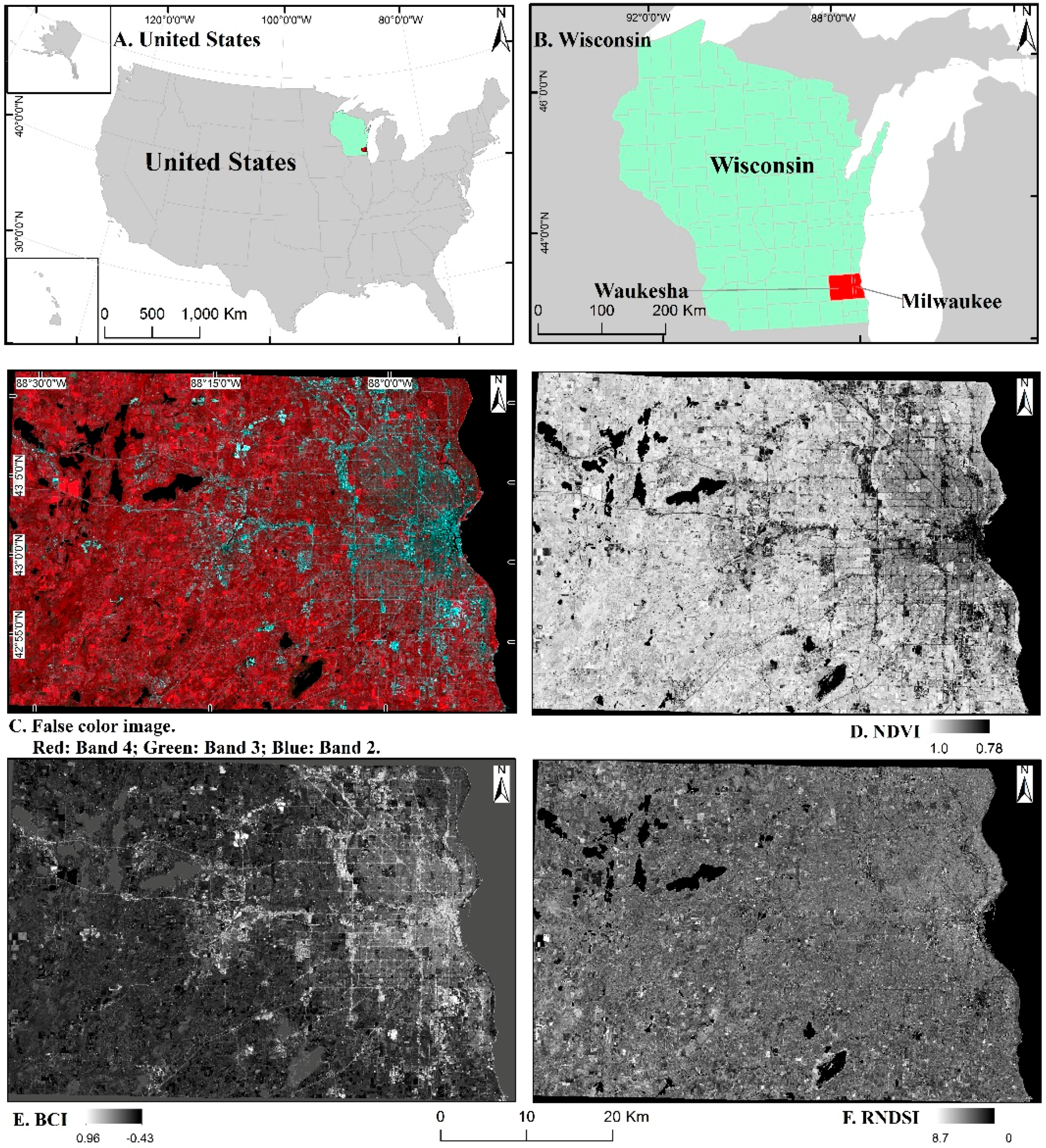
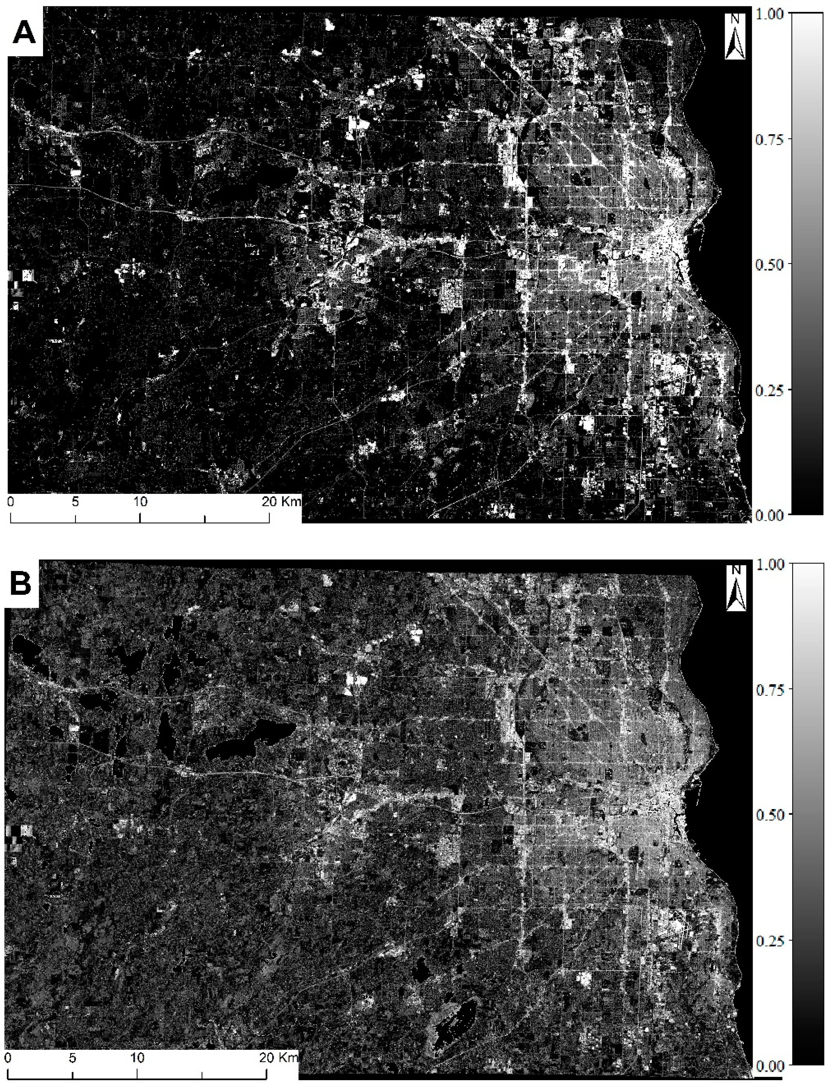
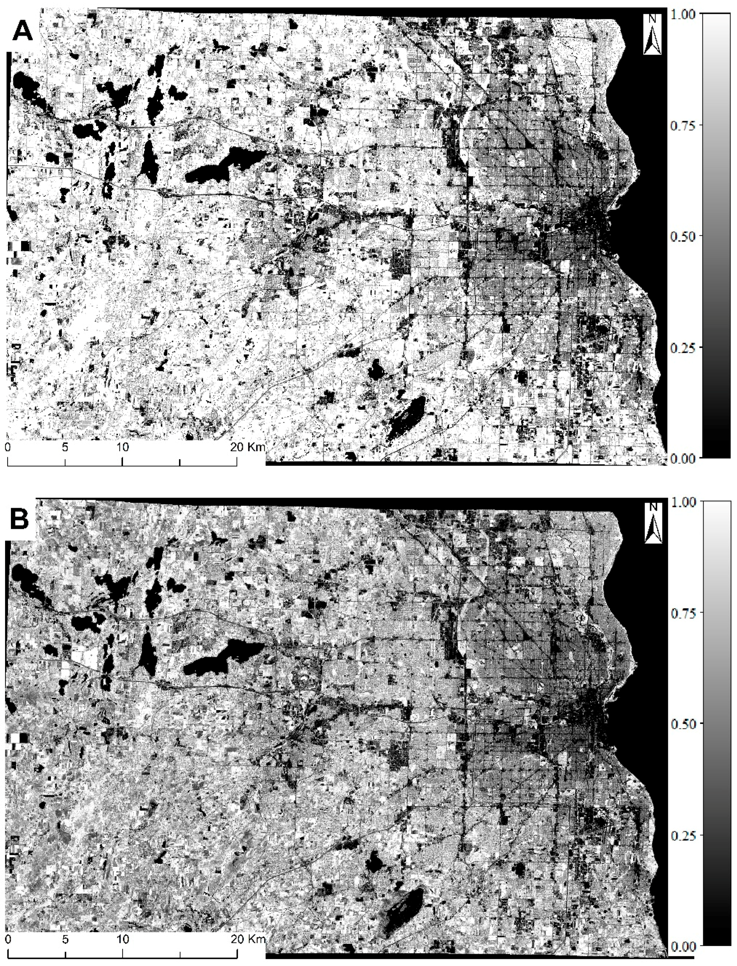
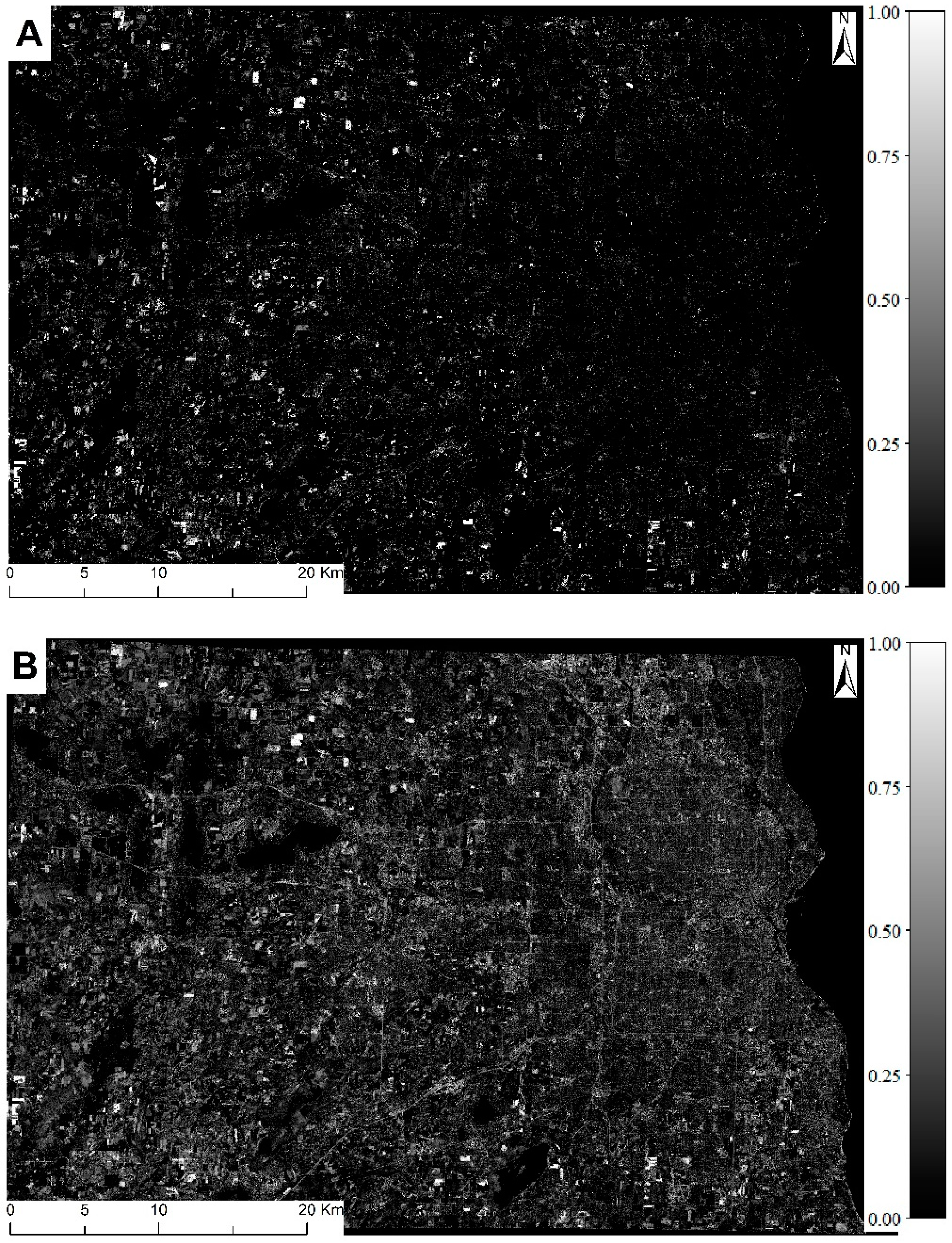
Two counties (Figure 1): Milwaukee and Waukesha in Wisconsin, United States, were selected as the study area. Geographically, both of these two counties are located in the Great Lakes Region with a humid continental climate. They cover about 2665 km² with a population of 1.3 million [23]. Milwaukee is dominated by urban and suburban land uses (e.g., commercial, residential, and industrial areas, etc.), while Waukesha is majorly covered by suburban and rural lands (e.g., farmland and forest). A large amount of ISA, bare soil, and vegetation exist in this study area, making it an ideal site for examining the effectiveness of the proposed C-MESMA model.

A scene of Landsat 7 Enhanced Thematic Mapper plus (ETM+) image (path 23, row 30) acquired on 11 September 2001 was used as the primary data. Six spectral bands (except the thermal band) with a spatial resolution of 30 m were utilized for C-MESMA. Digital numbers (DNs) of the image were converted into calibrated radiance image using the Landsat calibration model provided by ENVI, a commercial remote sensing image processing software. An atmospheric correction model, Fast Line-of-sight Atmospheric Analysis of Spectral Hypercubes (FLAASH) (Atmospheric Model: Mid-Latitude Summer, Aerosol Model: Rural, Aerosol Retrieval: 2-Band (K-T), Output Reflectance Scale Factor: 1), was applied to accurately compensate for atmospheric effects [24]. A Digital Orthophoto Quarter Quadrangle (DOQQ, Scale: 1:24,000) image of Milwaukee and Waukesha (13 April 2000) was utilized as the reference data to evaluate the performance of supervised classification and MESMA result. Water areas were masked with a supervised classification method before applying C-MESMA. All the images were re-projected to the Universal Transverse Mercator (UTM) with zone 16 and WGS84 datum.

3. Methods

C-MESMA includes two processes: supervised classification and MESMA (see Figure 2). Especially, supervised classification comprises the spectral indices generation and layer stacking, while MESMA contains subpixel unmixing (MESMA) and fraction image merging. Three spectral indices, normalized difference vegetation index (NDVI) [25], biophysical composition index (BCI) [26], and ratio normalized difference soil index (RNDSI) [27], were calculated and stacked with the Landsat reflectance image. Spectral characteristics of all land cover classes were expected to be enhanced by adding these three spectral indices [28]. Then, a support vector machine (SVM) was applied to the stacked image with six classes of elaborately-selected training samples. They were selected with reference to the DOQQ image to avoid the potentially-mixed pixels and to validate the correctness of the sample. These training samples contain three pure land cover classes: ISA (60 samples), soil (37 samples), and vegetation (60 samples), and three mixed land cover classes: vegetation-ISA (60 samples), vegetation-soil (60 samples), and vegetation-ISA-soil (26 samples). The ISA-soil land cover type was merged into the class of vegetation-ISA-soil as very few pixels belong to the ISA-soil land cover type. The whole study area was partitioned into six layers based on the results of SVM. Since the land cover classes of ISA, vegetation, and soil were considered as pure pixels, they were not involved in the unmixing process. Instead, a fraction value of one was assigned to the corresponding class directly. MESMAs were applied to the three mixed land cover classes with corresponding spectral libraries. Three fractional maps of ISA, vegetation, and soil were finally produced through merging the pure land cover classes, resulting from the SVM and the fraction images acquired from MESMA. Figure 2 shows the flowchart of the C-MESMA.

3.1. Supervised Classification

Spectral indices have been widely applied to remote sensing imagery to achieve better performances for image classification and visual interpretation [29]. In this paper, we applied this strategy to emphasize the spectral signatures of different land cover classes, aiming to mitigate spectral confusion between high albedo ISA and dry soil, low albedo ISA, and water, as well as shadow and water covers.

Three spectral indices, including biophysical composition index (BCI), normalized difference vegetation index (NDVI), and ratio normalized difference soil index (RNDSI), were stacked into the original reflectance bands of Landsat image. BCI, which is calculated by a reexamination of a tasseled cap transformation, can enhance the ISA information in the urban/suburban area. This shows better performance by reducing the soil effect when compared to the normalized difference impervious surface index (NDISI) and normalized difference built-up index (NDBI) [26]. Normalized difference vegetation index (NDVI) is a spectral indicator that represents vegetation cover and condition. It is the most successful attempt to quickly identify vegetation areas and their “condition” from remotely-sensed imagery [25]. Further, RNDSI can suppress ISA and vegetation values, as well as highlight soil information [27]. With each of these indices, only one land cover can be emphasized while others are suppressed, leading to enhanced differences between land cover types. These three indices can be calculated from Equations (1)–(3).

$$BCI=\frac{(H+L)/2-V}{(H+L)/2+V}$$

(1)

where $H=\frac{TC1-TC{1}_{\min }}{TC{1}_{\max }-TC{1}_{\min }}$, $V=\frac{TC2-TC{2}_{\min }}{TC{2}_{\max }-TC{2}_{\min }}$, and $L=\frac{TC3-TC{3}_{\min }}{TC{3}_{\max }-TC{3}_{\min }}$.

TC1, TC2, and TC3 represent the first, second, and third component in the tasseled cap transformation.

$$NDVI=\frac{B_{NIR}-B_{RED}}{B_{NIR}+B_{RED}}$$

(2)

B_NIR and B_RED refer to the reflectance in near-infrared and red bands, respectively.

$$RNDSI=\frac{NNDSI}{NTC1}$$

(3)

where $NNDSI=\frac{NDSI-NDS{I}_{min}}{NDS{I}_{max}-NDS{I}_{min}}$, and $NTC1=H$. H has the same values in Equation (1) and the NDSI can be written as Equation (4):

$$NDSI=\frac{(band 7-band 2)}{(band 7+band 2)}$$

(4)

where band 7 and band 2 are the seventh and second bands of the Landsat TM/ETM+ image. X_max and X_min are the maximum and minimum values of corresponding bands respectively (e.g., NDSI_max and NDSI_min represent the maximum and minimum value of NDSI respectively).

SVM is a widely used approach for the classification of remotely sensed imagery [30]. Its objective is to find the hyperplane that separates the dataset into a predefined number of discrete classes in a fashion consistent with the training samples [31]. A large number of applications have shown that SVM can produce a better performance than other pattern recognition techniques, like maximum likelihood and neural network classifiers [30]. Therefore, a SVM classification method was adopted in this research. With these three spectral indices (see Figure 1), as well as six Landsat spectral bands, an SVM classification was performed to classify the image into six land cover classes, namely ISA, vegetation, soil, ISA-vegetation, vegetation-soil, and vegetation-soil-ISA. Training samples were acquired from the Landsat image with a careful check from the DOQQ image. In a total of 330 reference samples (55 samples for each class) were employed to calculate the confusion matrix and to evaluate the performance of SVM classification.

3.2. MESMA

3.2.1. Endmember Selection and Spectral Library Construction

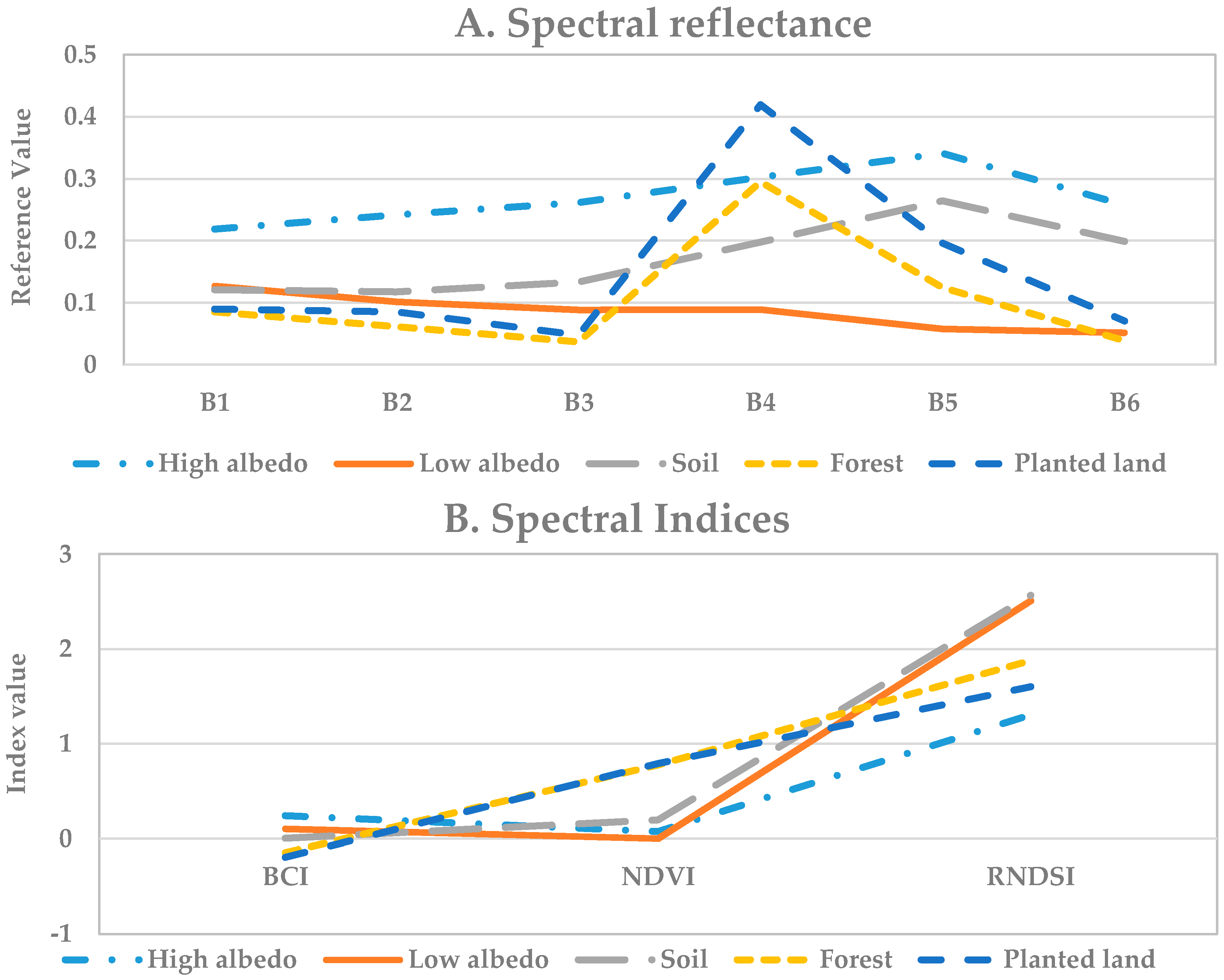
Endmember selection is a critical step for successfully implementing SMA [32]. Deciding the number of endmembers and their corresponding spectral signature is the first step to select proper endmembers. In this study, endmembers were extracted through choosing “pure” pixels in the Landsat image. The endmembers were selected with the following steps: (1) examining the entire study area carefully through visualizing the DOQQ image; (2) figuring out the number of endmembers in this study area; (3) overlapping the Landsat ETM+ image with the DOQQ image; (4) identifying regions containing corresponding endmembers; (5) extracting ETM+ pixels that locate in the center of each individual region; (6) comparing these selected pixels to the pixels of same location in the SVM image and removing erroneously-labeled pixels; and (7) averaging the spectra of selected pixels of each endmember and employing the mean spectrum as endmember. Finally, five endmembers—forest, planted lands, high albedo features, low albedo features, and soil—were selected to build the spectral library. As it is unnecessary to perform a MESMA for pure land cover types, three spectral libraries were constructed, each of which is corresponding to each mixed land cover class (e.g., ISA-vegetation, vegetation-soil, and vegetation-soil-ISA) (see

Table 1. Spectral libraries and endmembers.

Libraries (Number of Endmember)	Endmembers
ISA-Vegetation (4)	High albedo, Low albedo, Forest, Planted land
Vegetation-Soil (3)	Forest, Planted land, Soil
Vegetation-Soil-ISA (5)	High albedo, Low albedo, Forest, Planted land, Soil

). Spectral reflectance values and spectral indices of each endmember are shown in Figure 3.

3.2.2. Model Construction

SMA assumed that a spectrum of a mixed pixel is combined by several endmembers’ spectra. It centers on applying a mathematical method to derive the fraction of each endmember. Linear SMA is one of the most commonly used SMA with the assumption that each land cover was combined, linearly, to form a pixel’s spectrum. LSMA can be expressed as Equation (5):

$$R_i={\displaystyle \sum _{k=1}^n{f}_k}{R}_{ik}+E{R}_i$$

(5)

where i = 1,…, m (m: number of bands); k = 1,…, n (n: number of endmembers); R_i is the spectral reflectance of band i; f_k is the proportion of endmember k within the pixel; R_ik is the known spectral reflectance of endmember k within the pixel on band i; and ER_i is the estimation error for band i. A fully-constrained least squares solution [24] was applied which assuming that the following two conditions are satisfied simultaneously: ${\displaystyle \sum _{k=1}^n{f}_k}=1$, and $0\le f_k\le 1$.

Although simple, LSMA is not suitable for complex urban environments with a large number of manmade materials. As only one endmember is allowed for each cover type, LSMA cannot adequately address spectral variability in complex urban areas [11,33,34,35]. Multiple Endmember Spectral Mixture Analysis (MESMA), which was proposed by Roberts [14], is an improved method accounting for within-class and between-class spectral variability [25]. The number of spectra is not limited in the spectral library and the endmember combination can vary from pixel to pixel, which effectively solves the spectral variability issue in LSMA. In this study, MESMA was applied to three mixed land cover types with their corresponding spectral libraries. RMSRE (Equation (6)) was utilized as the parameter to select the best-fit endmember model. In other words, it is used to evaluate the performance of the endmember combination. Here, we used the abbreviation of RMSRE in order to differentiate the root mean square error (RMSE) which was utilized for assessing the accuracy between estimated and reference fractions in MESMA results:

$$RMSRE=\sqrt{{\displaystyle \sum _{i=1}^N\frac{E{R}_i{}^2}{N}}}$$

(6)

where ER_i is estimation error of band i, which was calculated using Equation (5), and N is the total number of bands.

Generally, a model with more endmembers may lead to a lower RMSRE when compared to that with fewer endmembers. However, inappropriate endmembers may be included and, therefore, lead to erroneous estimation of fractional land covers. To address this problem, a model with fewer endmembers may be selected as the best-fit model if, when compared to the model with a larger number of endmembers, the RMSRE’s difference is small (e.g., less than 0.1) [21]. With land cover fractions derived from MESMA, vegetation fractions were derived as the summation of those of forest and planted lands, and ISA fractions were calculated through adding the fractions of low-albedo and high-albedo materials. Finally, the fractional land cover maps were generated through combining the fraction images resulted from SVM and MESMA.

3.3. Accuracy Assessment

Accuracy assessment is a required procedure for evaluating the model performance. Traditional accuracy assessment methods, such as a confusion matrix, Kappa coefficient, and overall accuracy, however, are not applicable for subpixel-based mixture analysis [36,37,38]. The most commonly used approach is root mean square error (RMSE), which compares the fraction values between reference and modeled results. Reference fraction values were measured from the DOQQ imagery in the same sample sites as samples in the MESMA result. In this study, only the fraction of ISA is chosen to be analyzed, owning to the facts that (1) soil and vegetation change extremely between seasons and (2) the acquisition date of DOQQ image was not perfectly matched to the date of the Landsat image. Therefore, accuracy analysis of vegetation and soil was ignored. RMSE can be written as Equation (7):

$$RMSE=\sqrt{\frac{{\displaystyle \sum _{i=1}^N{({\widehat{X}}_i-X_i)}^2}}{N}}$$

(7)

where ${\widehat{X}}_i$ is the modeled ISA fraction value of sample i, and $X_i$ is the reference ISA fraction value of sample i, and N is the number of samples.

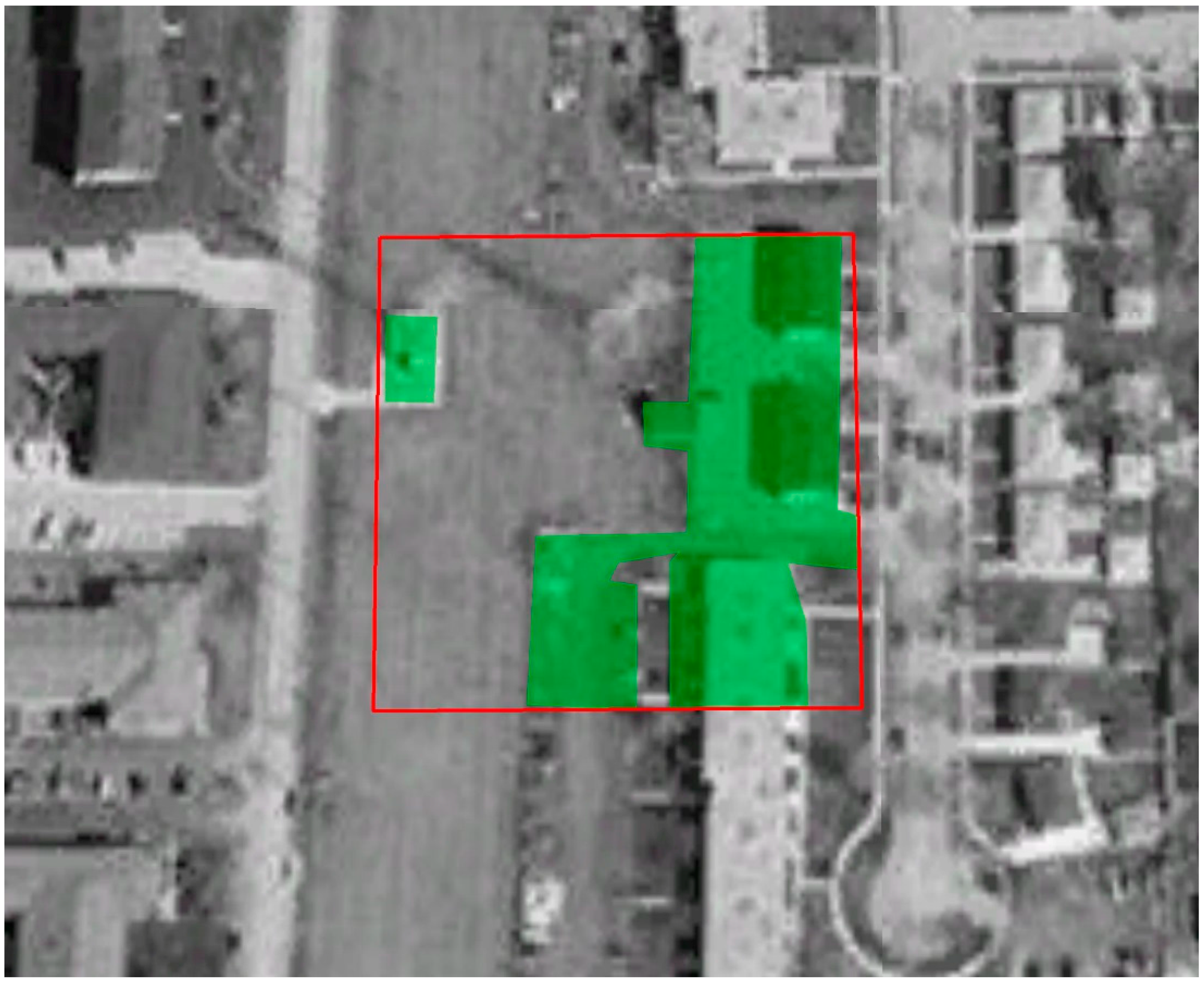
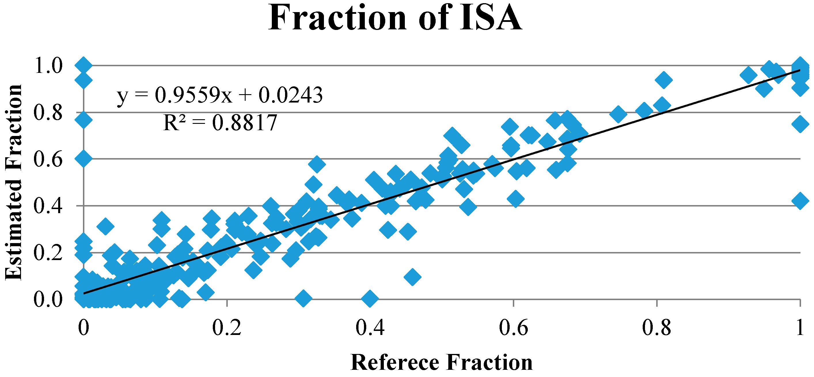
In total, we selected 351 samples (vegetation: 62, soil: 20, ISA: 32, vegetation-soil: 37, vegetation-ISA: 128, and vegetation-ISA-soil: 72) using a stratified random strategy. Each sample was designed as 90 m × 90 m (3 pixels × 3 pixels in the Landsat image) to mitigate the impact of geometric errors introduced in data acquisition and projection transformation. 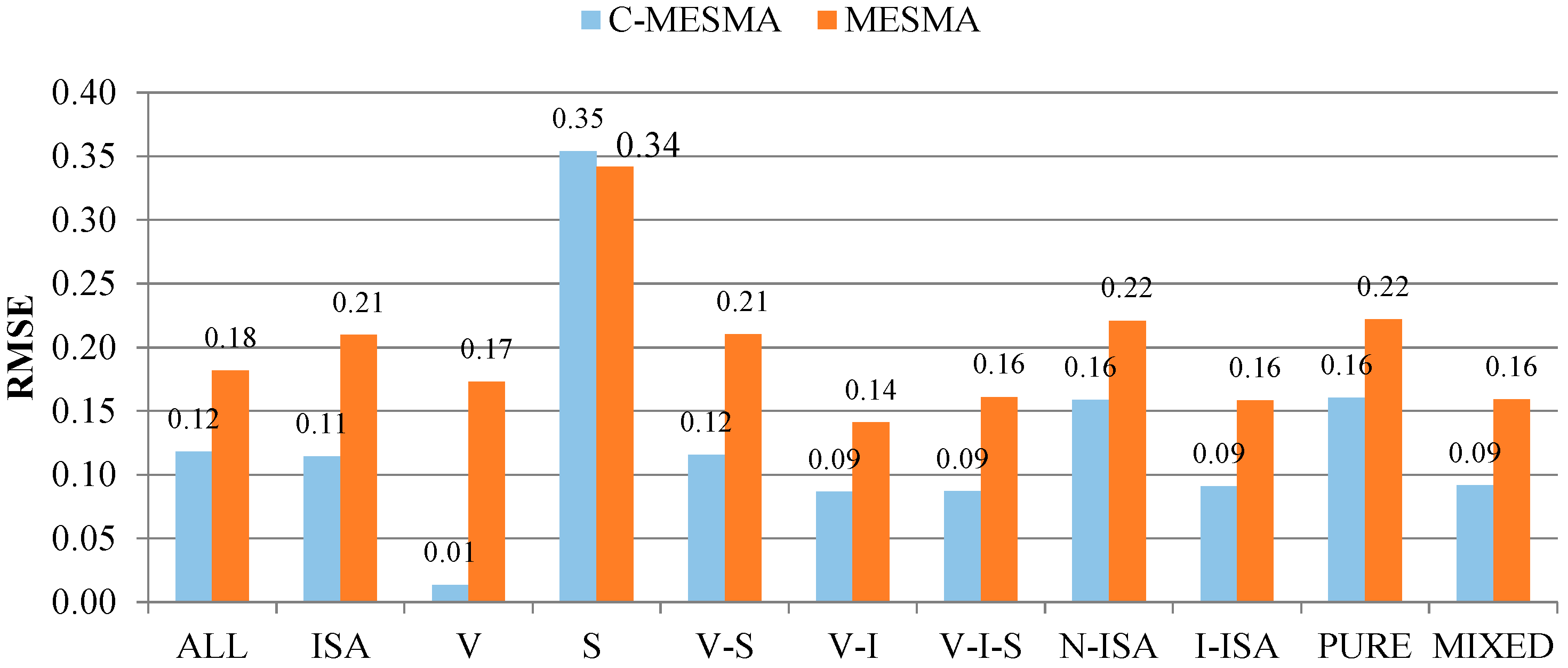Fractions of ISA in the DOQQ image were extracted by digitizing ISAs within the sample (See Figure 4). For examining the performance of C-MESMA, we identified eleven categories, including all samples, ISA samples, vegetation samples, soil samples, vegetation-soil samples, vegetation-ISA samples, vegetation-ISA-soil samples, ISA-excluded samples, ISA-included samples, all pure land cover type samples, and all mixed land cover type samples. The accuracy of each category was also compared to the corresponding results of the traditional MESMA.

4. Results

4.1. SVM Classification

With SVM, the whole study area was classified into six land cover classes. Classification results (see Figure 5) indicate that ISA areas were mainly located in Milwaukee County, especially in the downtown area and large shopping malls. Vegetation was primarily distributed in the southern region. Soil, which was much more dispersed than vegetation and ISA, was significantly distributed in the rural area. Vegetation-ISA was the major land cover type in the residential area, which was located outside the central business district (CBD) region. Vegetation-soil areas mainly occupied the farmland area. Vegetation-ISA-soil areas were mainly close to roads and residential lands.

The confusion matrix and Kappa statistics were calculated to illustrate the accuracy of SVM classification. With the overall accuracy of 87.58% and Kappa coefficient of 0.85, SVM result is acceptable for further analysis. Details of classification accuracy are shown in

Table 2. Confusion matrix of SVM classification.

Classified Data	Reference Data
	ISA	V	S	I-V	V-S	V-I-S	Total	User Acc. (%)
ISA	54	0	6	2	1	1	64	84.38
V	0	55	0	2	12	0	69	79.71
S	0	0	43	0	1	0	44	97.73
I-V	0	0	3	50	7	1	61	81.97
V-S	0	0	3	1	34	0	38	89.47
V-I-S	1	0	0	0	0	53	54	98.15
Total	55	55	55	55	55	55	330
Prod. Acc. (%)	98.18	100	78.18	90.91	61.82	96.36
Overall Accuracy = 87.58%			Kappa Coefficient = 0.85

Note: ISA, V, S, I-V, V-S, and V-I-S mean classes of impervious surface area, vegetation, soil, impervious surface-vegetation, vegetation-soil, and vegetation-impervious surface-soil, respectively.

.

4.2. MESMA

Five endmembers, including planted land, forest, high albedo, low albedo features, and soil, were selected to build the spectral libraries of corresponding land cover types. For each mixed land cover type (i.e., ISA-vegetation, vegetation-soil, and vegetation-soil-ISA), an individual MESMA was applied to estimate the fraction of these endmembers. Subsequently, the ISA fractional map was generated through adding the fractions of low and high albedo features for these mixed land cover types, and merging the fractional maps for the pure land cover classes (see Figure 6A). Similarly, the vegetation fractional map was derived through adding the fractions of forest and planted lands for the mixed land cover types, as well as merging those for the pure classes (see Figure 7A). Finally, the soil fractional map was created through merging the fractional soil maps for the mixed and pure soil fractional maps (see Figure 8A). For a better comparative analysis, the resultant fractions of ISA, vegetation, and soil generated from the traditional MESMA with the same endmembers, data source, and unmixing algorithm were also shown in Figure 6B, Figure 7B and Figure 8B.

Visualization of the ISA fractional map (Figure 6A) suggests that high percentage of ISAs (%ISA) is concentrated in the CBD of Milwaukee City and large shopping malls. Additionally, major roads and highways also contribute to high values of %ISA, as well. Medium %ISA mainly dominated residential areas surrounding the CBD of Milwaukee. Comparatively, a consistent spatial pattern of ISA distribution was found with C-MESMA and MESMA. Major differences, though, lie in the ranges of the estimated %ISA values in urban and rural areas. With C-MESMA, higher %ISA values were obtained in urban areas, while lower %ISA values were derived in rural areas (see Figure 6A,B). Taking rural areas as an example, the %ISA of planted lands and forest areas is near zero with C-MESMA, while the values are approximately 20% with MESMA. This overestimation is primarily due to the mistaken inclusion of ISA endmembers in MESMA. Conversely, for urban areas, %ISA values are higher with C-MESMA, mainly due to the exclusions of soil members.

In addition to %ISA, there are also differences in terms of the estimation of vegetation and soil fractions (see Figure 7 and Figure 8). It appears that, with C-MESMA, the fractions of vegetation are relatively higher when compared to those derived from MESMA (see Figure 7). For soil fractions, it appears that less soil was estimated in urban Milwaukee, and a higher amount of soil was derived in rural areas with C-MESMA (see Figure 8).

4.3. Accuracy Assessment and Comparative Analysis

In addition to the visual examinations of the fractional maps of ISA, vegetation, and soil, a quantitative accuracy assessment was also applied. As discussed in Section 3.3, we examined the accuracy of %ISA estimation for eleven groups of samples, namely ISA, vegetation, soil, vegetation-soil, vegetation-ISA, vegetation-ISA-soil, ISA-excluded, ISA-included, all pure land cover types, and all mixed land cover types. RMSE of each group of samples was calculated for both C-MESMA and MESMA (see Figure 9). Results revealed that, for almost all categories except soil, RMSE values of C-MESMA were significantly lower than those of MESMA. With C-MESMA, the overall RMSE was 0.12, which is significantly lower than 0.18 with MESMA. RMSE of soil with C-MESMA (0.35) was slightly higher than that in MESMA (0.34). Of course, both of them were relative high compared to those of the other land cover types, indicating the difficulty of separating ISA and bare soil. In addition to accuracy assessment for all samples, with C-MESMA, RMSEs of vegetation, vegetation-soil, vegetation-ISA-soil, ISA-included, and mixed land cover samples were less than 0.1. Especially, the RMSE of vegetation land cover type was 0.01, meaning that almost all fractions in the C-MESMA matched perfectly with the reference data. RMSEs in the corresponding land cover types of MESMA were at least 0.05 higher than those with C-MESMA. The RMSEs of ISA, vegetation-soil, ISA-excluded, and pure pixels with C-MESMA were a somewhat higher, but their values were much lower than those with MESMA. In summary, these comparative analyses show that the performance of C-MESMA is better than MESMA for almost all land cover types in this research.

In order to further investigate the relationship between the estimated fractions in the result of C-MESMA and the reference data, a scatterplot was employed to display their correlation (Figure 10). A trend line, which indicates the linear relationship, showed that the slope was close to one, and the R-squared value was 0.88, indicating a significant correlation between the estimated fractions and the reference values.

5. Discussion

Although MESMA allows endmembers and their combinations to vary from pixel to pixel, the “best-fit” model may still choose an inappropriate endmember set, mainly due to inter-class and intra-class variations of the endmember spectra. As a result, erroneous fractional estimates of land covers may be obtained due to the mistakenly inclusion or exclusion of endmembers in the model [17]. Unfortunately, few SMA/MESMA techniques have addressed this problem in previous studies, and most scholars ignore the fact that endmembers are not equally distributed, spatially. Franke et al. [21] and Liu and Yang [22] did partially address this limitation by dividing the whole study area into several regions, which, to some degree, restricts the distribution of endmembers. Their methods also have limitations. Mixed pixels cannot be fully separated with the classes of impervious surface and non-impervious surface areas/vegetation, thereby leading to the misclassification in the resultant segmented images. To accommodate the mixed pixel problem, we introduced mixed land cover types in the SVM classification. That is, the entire study area is classified into three pure land cover types (e.g., ISA, soil, vegetation) and three mixed land cover types (e.g., ISA-vegetation, soil-vegetation, and ISA-soil-vegetation). With this approach, a major limitation of pixel-based hard classifications, that only one land cover class can be assigned to a pixel [13,20], has been successfully addressed by allowing the assignment of pixels into a mixed land cover class.

C-MESMA not only constrains the spatial distribution of endmembers but also improves the computational efficiency. An issue of the traditional MESMA approach is the employment of a global spectral library for an entire study area. Although it can address the inter-class and intra-class spectral variability to some degree [7], the criteria of selecting the best-fit endmember model still needs to be verified systematically, as it may include inappropriate endmembers. With C-MESMA, three separated spectral libraries are built based on corresponding mixed land cover types. On the one hand, the distribution of endmembers is restricted in the corresponding land cover classes, and inappropriate endmembers are excluded from the unmixing model. As an example, for the vegetation-ISA land cover type, only endmembers of vegetation and ISA are considered, and soil is effectively excluded in the model. With this advantage, the over-estimation of soil in urban areas was effectively addressed in the study area. On the other hand, with the reduction of irrelevant spectral endmembers, the number of spectral signatures decreases significantly, which improves the computational efficiency during the unmixing process. Moreover, with a lower number of spectral signatures in the spectral libraries, C-MESMA may also improve the computational efficiency. Some researchers have attempted to improve the computational efficiency by separating the entire spectral library into several libraries. Each of these libraries only contains spectra of one land cover class [39]. Computational time may be reduced with this strategy. However, only one spectrum of every land cover class can be included in each endmember combination, thereby reducing the performance of addressing the within-class variability. For instance, impervious surface areas commonly contain two types of features, high albedo and low albedo surface features [40]. These two types of land surface features are always close to each other, especially in downtown areas. Misclassification may appear if only one of them is contained in the endmember combination models. On the contrary, C-MESMA considers all the spectra as potential endmembers. The reduction of spectral library size is attribute to the constraint of corresponding land cover types derived from the SVM classification. Additionally, pure land cover classes resultant from the SVM are excluded from further spectral unmixing, which further reduces the computation time.

Although with advantages, C-MESMA cannot adequately address the confusion between soil and ISA. This is because that the spectral signatures of sandy soil are highly similar to those of high albedo ISA. As a result, fractions of dry soil are overestimated. Nonetheless, most of the sandy soil is located in the developing regions or the factory areas. These areas, to a certain degree, are classified as urban land uses.

6. Conclusions

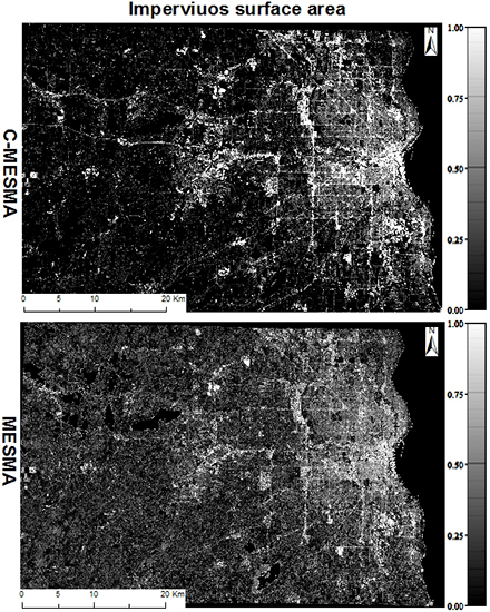
A novel approach called land cover-class based multiple endmember spectral mixture analysis (C-MESMA), which combines the pixel-based supervised classification and MESMA, is proposed to extract the fractions of the ISA, vegetation, and soil. The C-MESMA, which firstly partitions the land cover into three pure land cover classes (vegetation, impervious surface area, and soil) and three mixed land cover types (ISA-vegetation, soil-vegetation, and ISA-soil-vegetation), then estimates the fractional coverages of mixed land cover classes using MESMA, is a promising and efficient method to prevent the appearance of inappropriate endmembers. Mixed pixels are being classified as an independent land cover class, breaking through the limitation of pixel-based classification that every pixel should belong to a pure land cover class. A fraction value of one is assigned to the corresponding pure land cover classes while the mixed land cover classes are unmixed using MESMA with their corresponding spectral libraries, not only improving the computational efficiency but also avoiding overestimating the fraction of an improper endmember and underestimating the suitable endmember’s fraction. Accuracy assessment and quantitative/qualitative analyses prove the significantly better performance of C-MESMA when compared to MESMA.

Admittedly, the classification accuracy of soil is relative low. A major reason is that the spectra of sandy soil and ISA are almost the same, which cannot be well distinguished through the SVM and MESMA. Additional information about soil should be included to reduce the mixture of sandy soil in the future. Moreover, the number of land surface features identified in this research is limited, and more details of specified materials in urban environment are expected to be distinguished in future experiments with the help of hyperspectral data.