Continent-Wide 2-D Co-Seismic Deformation of the 2015 Mw 8.3 Illapel, Chile Earthquake Derived from Sentinel-1A Data: Correction of Azimuth Co-Registration Error

Abstract

In this study, we mapped the co-seismic deformation of the 2015 Mw 8.3 Illapel, Chile earthquake with multiple Sentinel-1A TOPS data frames from both ascending and descending geometries. To meet the requirement of very high co-registration precision, an improved spectral diversity method was proposed to correct the co-registration slope error in the azimuth direction induced by multiple Sentinel-1A TOPS data frames. All phase jumps that appear in the conventional processing method have been corrected after applying the proposed method. The 2D deformation fields in the east-west and vertical directions are also resolved by combing D-InSAR and Offset Tracking measurements. The results reveal that the east-west component dominated the 2D displacement, where up to 2 m displacement towards the west was measured in the coastal area. Vertical deformations ranging between −0.25 and 0.25 m were found. The 2D displacements imply the collision of the Nazca plate squeezed the coast, which shows good accordance with the geological background of the region.

1. Introduction

On 16 September 2015, an earthquake of Mw 8.3 [1] occurred 48 km from the west of Illapel, Chile, causing extensive damages to the area and leading to a large tsunami [2]. In this earthquake, at least 15 people died, 34 people injured, and tens of thousands of people became homeless. A total of 13 aftershocks ≥ Mw 6.0 soon afterwards occurred within 200 kilometers around the epicenter [1]. Chile is in one of the most earthquake-prone regions in the world and has been attacked by more than a dozen of quakes ≥ Mw 8.0 (see Figure 1) since 1900. The Nazca plate is moving at an average velocity of 74 mm/year east-northeast, and subducting beneath the continent at the Peru-Chile Trench of the South American plate [3]. The 2015 Mw 8.3 Illapel earthquake occurred as the result of thrust faulting on the interface between the Nazca and South American plates in central Chile [1,4]. The USGS report [4] shows that the epicenter of this event locates at 31.57°S, 71.654°W with a focal depth of about 25 km, and its dimension is typically about 230 × 100 km (length × width).

Currently, few geodesy measurements (such as GPS, spirit leveling) are available for scientists to further study this event. Thanks to a new generation of SAR systems, such as the Sentinel-1A (S1A) [5,6] equipped with the Terrain Observation by Progressive Scans (TOPS) [7], the continent-wide Interferometric Synthetic Aperture Radar (InSAR) measurements becomes possible. Previous studies [8,9,10,11,12] have demonstrated the capability and great potential of S1A TOPS in ground surface deformation monitoring. In contrast to the conventional strip-map or ScanSAR data, multiple consecutive S1A TOPS frames (defined by ESA, where one zip file of S1A TOPS data distributed in Scihub [13] denotes a single frame) can generate long seamless strip data which is 250 km wide. Thus, it extremely benefits the study of large continent-wide event, such as the 2015 Mw 8.3 Illapel earthquake.

The S1A TOPS, as a new mode of InSAR, also has some key technical issues that need further study, especially for co-registering multiple S1A TOPS data frames. The Doppler Centroid of TOPS SAR data varies strongly along tracks, so a co-registration accuracy of at least 0.001 SLC pixel is required to eliminate the effect [7]. Currently, the Spectral Diversity (SD) [14] method and the enhanced SD (ESD) [15], implemented in GAMMA [16] or GMTSAR [17], could perform well for a single frame data case, but cannot resolve the problem of co-registering multiple S1A TOPS data frames well.

In this study, we firstly proposed an improved Spectral Diversity (ISD) method to co-register the multiple S1A TOPS Interferometric Wide Swath (IWS) data frames. We then map the co-seismic LOS deformation associated with the 2015 Mw 8.3 Illapel earthquake using both ascending and descending S1A data and the methods of D-InSAR and Offset Tracking, respectively. Subsequently, the D-InSAR and Offset Tracking measurements are assessed in terms of precision and used together to retrieve the east-west and vertical co-seismic deformations of this earthquake. Finally, we discussed implications of ISD co-registration method and co-seismic measurements, as well as the potential contribution of the S1A data to further continent-wide event studies.

2. ISD Method for Co-Registering Multiple S1A TOPS Frames

2.1. ISD Method

Compared with the conventional strip-map InSAR, the TOPS mode InSAR has difficulty in azimuth co-registration due to a strong azimuth-variant Doppler centroid [7]. The interferometric phase bias caused by the Doppler centroid induced azimuth mis-registration (or azimuth offset) can be expressed as [7,18]:

$$∆\varphi =2\pi \cdot f_{DC}\cdot ∆d_{azi}/PRF,$$

(1)

where $f_{DC}$ is the Doppler centroid of the target point, $∆d_{azi}$ is the azimuth co-registration error, and PRF is the Pulse Repetition Frequency of focused SLC data. We should note that $f_{DC}$ varies linearly within a TOPS burst in the along-track dimension. Thus, a constant $∆d_{azi}$ will produce a series of azimuth phase ramps imposed onto an interferogram, resulting in phase discontinuity (or phase jump) on the burst interface [19].

To suppress the phase jump at burst overlap to ±1.5°, a co-registration accuracy of at least 0.001 SLC pixel is required [7,14]. Currently, an overall mis-registration error is usually corrected with constant azimuth offset $∆d_{azi}$ (see Equation (1)) based on the method of SD [18] or ESD [14]. For a single S1A IWS frame [13], which contains three sub-swaths and in each sub-swath there are typically nine burst, the number of burst is small (about 3 × (9 − 1) = 24 of burst overlaps), and these conventional methods can work well. However, conventional methods with a constant correction would be ineffective in the case of multiple consecutive S1A TOPS frames [20], because large variations of the Doppler centroid will result in considerable variations of azimuth mis-registration (or azimuth offset) for long imaging duration. More importantly, obvious phase jump would also occur on overlap area between burst, especially at the ends of the long data taken. In order to address this problem, an improved Spectral Diversity method is proposed in this study. Rather than treating $∆d_{azi}$ as a constant, the new method compensates the variation of the azimuth mis-registration by a linear model:

$$∆d_{azi}=∆d_{azi}^0+k\cdot t,$$

(2)

where $∆d_{azi}^0$ is the intercept, $k$ is the change rate of azimuth mis-registration error, and $t$ is the acquisition time difference between the current and the first SLC line. By substituting Equation (2) into Equation (1), one gets:

$$∆\varphi \cdot s=∆d_{azi}^0+k\cdot t,$$

(3)

where $s=\frac{PRF}{2\pi \cdot f_{DC}}$ is a scale factor converting phase to SLC azimuth offset. Given N observations (N is the quantity of burst overlaps) we get a linear system in matrix form:

$$L=B\cdot x,$$

(4)

where $x={[∆d_{azi}^0,k]}^T$ is the unknown vector, and $B$ is the design matrix:

$$B=\left[\begin{array}{ll}1& t_1\\ ⋮& ⋮\\ 1& t_N\end{array}\right].$$

The observation vector $L={[L_1,L_2,\cdots ,L_N]}^T$, where $L_i=∆{\varphi }_i\cdot s_i$ $(i=1,\cdots ,N)$ is the azimuth offset of the i-th burst overlap, with $∆{\varphi }_i$ being the average of the phase differences of the current and the next burst interferogram of the i-th burst overlap and $s_i=\frac{PRF}{2\pi \cdot f_{DC}^i}$ being the scale factor of i-th burst overlap.

When N > 2, Equation (4) becomes over-determined problem. To resolve the parameters $x$, we use an iterative weighted least square estimator [21,22,23], to account for possible gross error in observation vector $L$. When the estimation of $x$ was obtained, the azimuth co-registration error for each azimuth line could be calculated by Equation (2) and used to refine the SLC resample look-up table in S1A TOPS SLC co-registration, which will be discussed in next section.

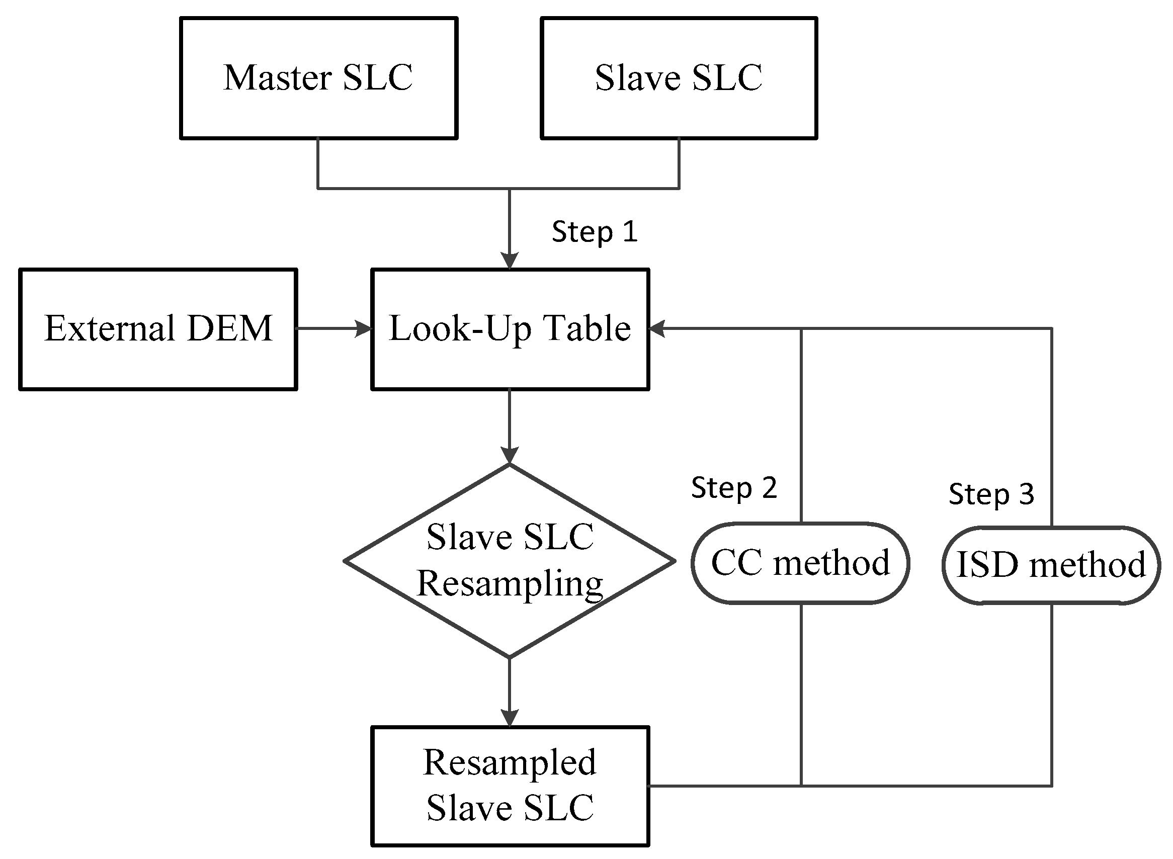
2.2. Procedure of S1A TOPS SLC Co-Registration with ISD

To meet the requirement and to counteract the topographic effect, the co-registration of wide-swath SLC images of S1A TOPS SLC [16] generally involves a sequentially DEM-assisted method (Step 1), conventional Cross-Correlation (CC) (Step 2) method, and a SD method (Step 3). Our ISD method can be easily embedded into the S1A SLC co-registration procedure for multiple S1A TOPS frames. Figure 2 shows the flow chart of the SLC co-registration, and the three key steps are summarized as follows.

• Step 1: initial co-registration. Estimate initial SLC images offset and set up SLC resampling look-up table [24] with orbital state vectors and an external DEM, e.g., SRTM DEM, and resample the slave SLC into master imaging geometry.
• Step 2: co-registration by the CC method. Determine the image offsets between master and the resampled slave SLC from Step 1 by the CC method, and use the image offsets to refine the look-up table. The original slave SLC is, again, resampled into master imaging geometry.
• Step 3: co-registration by ISD method. Calculate the mean phase differences of all bursts overlaps between the master and the resampled slave SLC from Step 2. Then the constant azimuth offset $∆d_{azi}^0$ and the change rate $k$ are resolved by ISD method. The look-up table is refined with an azimuth offset calculated from Equation (2) and the estimated parameters and, finally, output the resampled slave SLC using the ultimately-refined look-up table.

3. Data Processing

Ascending and descending tracks S1A data are used in this study (see Figure 1b). The details of the SAR data are shown in

Table 1. Information of SAR data.

Acquisition Date	Orbit Direction	Track	No. of Frame	No. of Total Burst	B⊥ (m)
24 August 2015	Ascending	18	2	36 1 = 2 × 2 × 9	70
17 September 2015	Ascending	18	2	36 = 2 × 2 × 9
26 August 2015	Descending	156	3	84 = 3 × 2 × 9	−116
19 September 2015	Descending	156	3	84 = 3 × 2 × 9

¹ No. of Total Burst = No. of Frame × No. of Sub-Swath per Frame × No. of Burst per Sub-Swath.

. The methods of Differential InSAR (D-InSAR) and Offset tracking will be exploited to estimate the Light of Sight (LOS) deformations. Finally, 2-D co-seismic displacement fields of this event will be derived.

3.1. Co-Registering Multiple Frames of S1A TOPS Data

The SAR co-registration follows the steps in Section 2.2. The 90 m SRTM DEM (v4.1) is used to estimate the initial look-up table [24] and remove the topographic phase. Thanks to the precise orbital state vector [6], an accuracy of a few pixels could be achieved [16] in the preliminary co-registration using orbital information. Then, the CC method is used to estimate the image offsets from evenly-distributed 64 × 192 (range × azimuth) tie-points with matching windows size of 128 × 256 (range × azimuth) pixels. All offsets are used to fit an offset polynomial that will subsequently be used to refine the look-up table. Due to limited accuracy of the CC method (~1/32 pixel) [25,26], the required co-registration accuracy of 0.001 SLC pixel could still not be achieved (see

Table 2. SLC co-registration accuracies.

Interferometric Pair	CC Method		ISD Method
	Azimuth (Pixel)	Range (Pixel)	Azimuth (Pixel)	Range (Pixel)
24 August 2015–17 September 2015	0.1170	0.0516	0.00104	---
26 August 2015–19 September 2015	0.0827	0.0425	0.00095	---

). Therefore, azimuth offset estimation with the proposed ISD is required for multiple S1A TOPS frames co-registration. We firstly calculated the observation vector $L$, the azimuth co-registration error, from each burst overlap. For descending data, three sub-swathes contain a number of (3 × (27 − 1) = 84) burst overlaps. Since some burst overlaps situate in low coherent area (average coherence < 0.75), such as sea or vegetation areas, 69 valid burst overlaps are used to fit the azimuth co-registration error. For ascending data, sub-swath 1 is located in the sea area, which is discarded directly. Sub-swathes 2 and 3 provide a total of 34 burst overlaps for fitting the azimuth co-registration error. The final fitted linear models are, respectively, $∆d_{azi}^{des}=0.01320-2.1698\times {10}^{-4}\cdot t$ and $∆d_{azi}^{asc}=0.01477+1.772\times {10}^{-4}\cdot t$ for descending and ascending tracks. The fitting results are also shown in Figure 3e. The azimuth co-registration accuracy with ISD is listed in Table 2, indicating that an accuracy of 0.001 SLC pixel has been achieved. Then the SLC resampling look-up table is refined by the fitted linear model. Finally, the slave SLC is precisely co-registered to the master SLC.

To demonstrate the effectiveness of our ISD method, the datasets are also co-registered with SD method implemented in GAMMA [16]. From comparisons in Figure 3a–d, we can see that obvious phase jumps still exist in the interferogram by the conventional SD method.

3.2. D-InSAR and Offset Tracking Processing

The TOPS D-InSAR processing, somewhat like traditional D-InSAR procedures [27], can be conducted after the SLC co-registration. As the Doppler centroid variations are different within bursts, we do not apply the azimuth common band filter in the interferogram [16]. The topographic phase is removed with 90 m SRTM, thus generating the differential interferogram, and multi-looking factors of 20 × 4 (range × azimuth) is applied to set the output result with a resolution of about 50 × 50 m. The improved adaptive phase noise filter [28] is utilized to smooth the interferogram. Subsequently, the smoothed interferogram is unwrapped by network programming-based phase unwrapping method [29]. Low coherent area (coherence ≤ 0.75) is masked out in the phase unwrapping process. Eventually, the LOS deformations from both the ascending and descending tracks are obtained (see Figure 4a,b).

Apart from the D-InSAR measurements, the Offset Tracking [19] measurements in the slant range and azimuth direction are also achieved by conventional CC method [25] using the co-registered SLC images. The sliding step size of offset estimate window is set to be 20 × 4 (range × azimuth) pixels to generate the same resolution result with D-InSAR. To reduce the noise, center weighted median filter [30] with a window size of 11 × 11 (range × azimuth) is employed to smooth the offset measurement, in which the correlation coefficient of the matching windows is used as the weight factor. From our offset tracking measurement implementation, we find that the azimuth deformation is difficult to be detected. This is also confirmed by Multiple-Aperture Interferometry (MAI) technology, whose expected accuracy for S1A TOPS IWS data is about 27 cm [25]. Thus, we do not use the azimuth offset measurements in our further study. The range offset measurements for ascending and descending orbits are shown in Figure 4d,e.

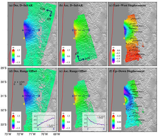
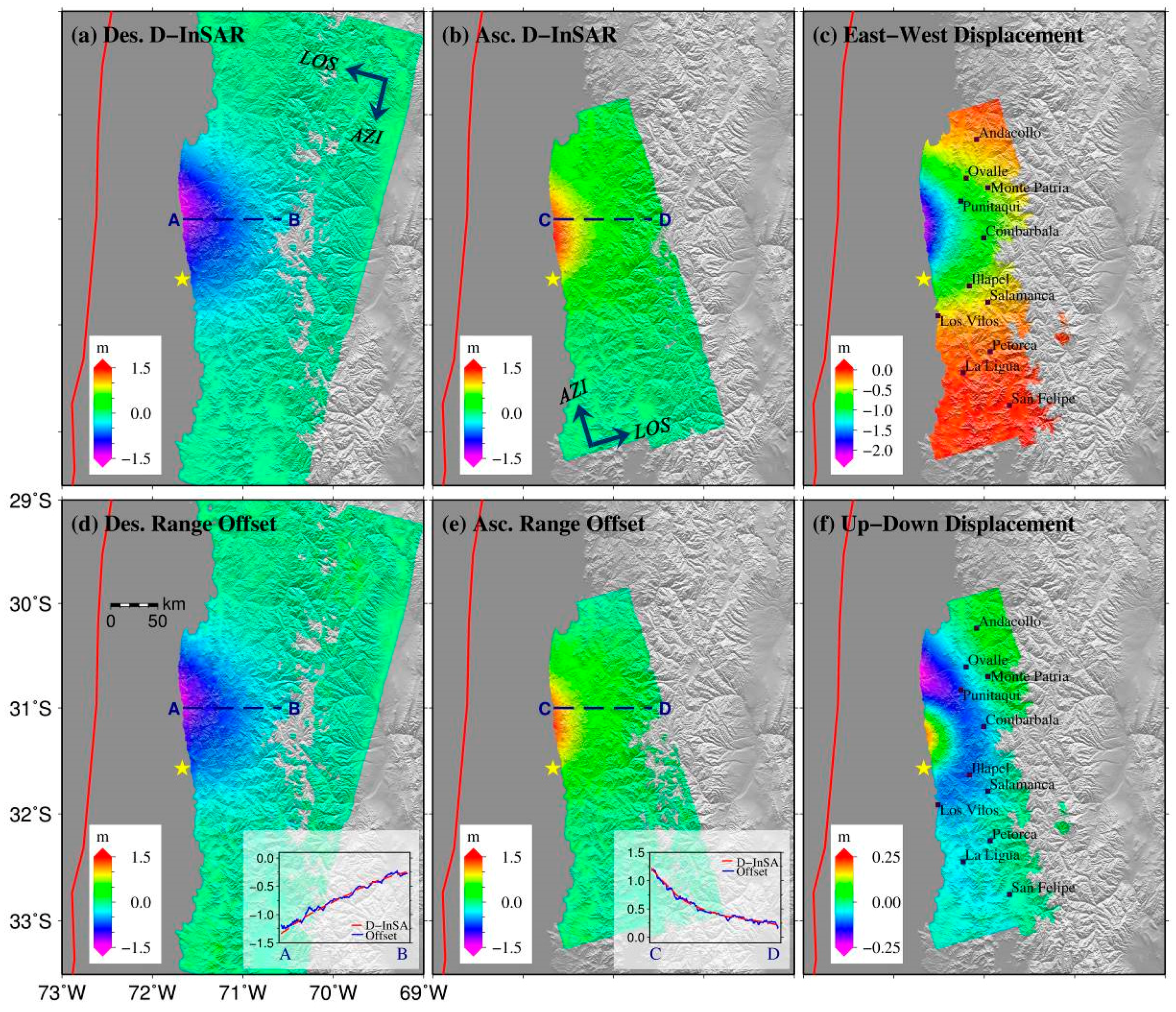
3.3. Precision Assessment and 2-D Displacement Retrieval

The precisions of both D-InSAR and Offset Tracking measurements are assessed by evaluating the local standard deviations (STDs) on sliding window with a size of about 1 × 1 km pixel-by-pixel [31]. The linear trend is fitted and subtracted from the sliding window to get stationary signals for calculating the STDs. The local STDs maps of the measurements from D-InSAR and Offset Tracking in the slant range are shown in Figure S1, which will be used as the weight factor to derive the 2D displacement of this earthquake.

Theoretically, three dimensional (3D) deformations [32] could be resolved with LOS and along-track measurements from two or more viewing geometries [33,34]. However, the north-south direction displacement is insensitive in D-InSAR measurements in general, and beyond the detectability of S1A TOPS IWS data in this earthquake in particular [25]. Thus, the north-south deformation is compromisingly neglected in this study. The unit projection vector of LOS deformation for ascending and descending orbits are $S_{asc}={[s_e,s_n,s_u]}^T={[-0.607,-0.170,0.755]}^T$and $S_{des}={[s_e,s_n,s_u]}^T={[0.608,-0.168,0.776]}^T$, respectively. By assuming the north-south deformation is null and exploiting the projection vectors $S_{asc}$ and $S_{des}$ to establish observation equation, two dimensional (2D) deformations, i.e., east-west and up=down (or vertical) are derived by combing the D-InSAR and Offset Tracking measurements from ascending and descending orbits [35]. We acknowledge that neglecting the north-south deformation will induce errors in the east-west and vertical deformation estimation, but for the Illapel earthquake it might be very slim, because the azimuth deformation itself is very small. The final 2D deformations are shown in Figure 4c,f.

4. Results

We got the co-seismic LOS deformations and the 2-D, i.e., east-west and vertical displacements with the elaborated data processing strategy presented in previous section. Figure 4a,d show the co-seismic LOS deformations extracted by D-InSAR and Range Offset Tracking with descending track InSAR data, and Figure 4b,e are the co-seismic LOS deformations with ascending track InSAR data. Due to the effect of decorrelation, there are still some areas along the Andes Mountains that has been masked out.

Comparing the D-InSAR and the Offset Tracking measurements, we can find that they have the same LOS deformation pattern and the same deformation magnitude, showing remarkably good agreement between each other. To make more detailed comparisons, the profiles along A-B and C-D are displayed as insets in Figure 4d,e. These results illustrate quite good consistency in the LOS D-InSAR and Offset Tracking measurements for S1A TOPS mode data. Comparing the D-InSAR measurements from both descending and ascending track, we can see that they have quite a similar deformation pattern, which implies that the horizontal displacement dominates the ground deformation; we can also see that most of the deformation with large magnitude locates on the upper part along profile A-B near the coast in descending track, while it is opposite in ascending track, implying that obvious vertical displacement has occurred and the upper part sank and the lower part uplifted.

Figure 4c shows the east-west displacement, where up to 2 m and towards the west occurred in the coastal area. Vertical displacement (Figure 4f) associated with the ground uplift and subsidence ranging between [−0.25, 0.25] m is also detected. It should be noted that east-west and vertical displacements are only calculated over the common area of all measurements (Figure 4a,b,d,e), which ensures that there are redundant observations for alleviating the effect of atmospheric [36] in the 2-D deformation inversion.

5. Discussion

To improve the accuracy of co-registering multiple S1A TOPS data frames, an ISD method is proposed and embedded into the S1A SLC co-registration procedure. Comparing with the conventional SD or ESD methods, the ISD method is more suitable for multiple S1A TOPS data frames co-registration by compensating the variation of azimuth co-registration error using a linear model. However, some issues shall be carefully settled to ensure the accuracy of ISD. Firstly, similar to the SD or ESD methods, the ISD method is subject to small azimuth offset measuring. The prerequisite for using ISD method is that the azimuth offset should be within ±0.75 SLC pixels [19] Therefore, the azimuth offset shall firstly be truncated to this limit by other methods before applying the ISD method, e.g., the conventional CC method. Secondly, as shown in Equations (1) and (2), the observation, i.e., azimuth co-registration error $∆d_{azi}$ on each burst overlap, relates linearly to the phase offset $∆\varphi$. To obtain a high coherent phase offset, the burst overlap’s phase difference of subsequent bursts shall be multi-looked with a large factor, e.g., 100 × 4 (range × azimuth) pixels and, subsequently, be filtered to reduce phase noise [28,31]. The multi-looking factor depends on the phase quality, and we found that a factor of 100 × 4 is empirically enough. Additionally, it should be noted that the north-south deformation would cause an azimuth offset [15] too, which will superimpose on the normal azimuth co-registration error. If only a part of burst overlaps have north-south deformation, our ISD method would automatically exclude those observations by an iterative weighted least square estimator [21], as those observations possibly manifest as gross errors with respect to the normal azimuth offset observations. Furthermore, given the prior information we could also manually remove the observations contaminated by north-south deformation, and the final ISD accuracy would be improved in such a situation.

The 2015 Mw 8.3 Illapel earthquake occurred on the interface between the Nazca and South American plates (see Figure 1). The co-seismic deformation of this earthquake is mapped with S1A TOPS data in this study. Comparing our results with those obtained by the European Space Agency’s Project on Sentinel-1 INSAR Performance Study with TOPS Data [37], we found that ours are continuous and clear, while their D-InSAR interferograms still have obvious phase jumps, similar to the results in Figure 3c, for both ascending and descending tracks. Affecting by the discontinuities of the D-InSAR measurements, their decomposed vertical displacement has considerable leap. All of these errors would provide false information for the interpretation of earthquake mechanism. On the contrary, there are no phase jumps in our results (see Figure 4a,b). In addition to the D-InSAR measurements, we also extract the Offset Tracking measurements in the LOS direction. Both D-InSAR and Offset Tracking LOS measurements show good consistency (see Figure 4a,b,d,e). This confirms that the SLC images have been precisely co-registered by our ISD method. In addition, we have derived the 2-D deformations from the LOS D-InSAR and Offset Tracking measurements. The results show that the coastal area moved westwards by up to 2 m, and the vertical displacement (see Figure 4f) associated with ground uplift and subsidence ranging between [−0.25, 0.25] m has also been detected. Additionally, by measuring the deformation area, we also found the dimension of the event is consistent with the result from USGS [4]. Additionally, the 2-D displacements, a recent study [38] has tried to recover the 3-D displacements of the event, in which they use the along-track interferometry [38] to measure the azimuth deformation. By comparing them, we found that our results are in line with theirs. However, the along-track measuring [38] can only be applied to the burst overlap region, which occupies only about 15% of the whole frame. While, for the non-burst overlap region, occupying about 85% of the frame, interpolation processes must be implemented, which will, of course, induce errors.

Chile is prone to earthquakes that have caused severe destruction in the past century. The Nazca plate moves to the east-northeast at a varying rate (approximately 80–65 mm/year from north to south) relative to a fixed South American plate, resulting in complex geologic processes along the Nazca subduction zone [1]. At the latitude of the 2015 Mw 8.3 Illapel earthquake, many massive earthquakes have occurred, including the 2010 Mw 8.8 Maule earthquake in central Chile [3,39]. The 2D results show that the coastal area has moved westwards by up to 2 m accompanying with a little vertical deformation. This implies the collision of the Nazca plate squeezed the coast and the east-west displacement dominating the co-seismic deformation. The result is in good accordance with the geological background of the region. All those measurements would benefit for the geophysical parameters inversion of the 2015 Mw 8.3 Illapel earthquake.

S1A satellite is now in normal on-orbit operation. As the first SAR satellite of Sentinel-1 constellation, S1A systematically acquires SAR image over land area with a revisit of 12 days in Europe and 24 days for other regions [40]. S1A is controlled to follow an orbital tube of 100 m radius [41], which guarantees short spatial perpendicular baseline. These two merits reduce the decorrelation, which has been demonstrated in previous studies [27]. As a C-band SAR system, S1A also has a limited detectable deformation gradient capability with D-InSAR technology [42]. However, the increasing slant range resolution (up to 2 m) enhances the detectability along the slant range with the SAR Offset Tracking method, and makes it a good supplement for D-InSAR measurement. Additionally, the S1A acquires data with a wide swath (250 kilometer wide for IWS mode), which would be more favorable to study continent-wide event than the conventional SAR satellite (<100 km), like the ENVISAT and the ALOS. The advantages of S1A for large earthquake study have been presented in this work. The advent of S1A will boost geo-hazard monitoring and crisis management [43,44].

6. Conclusions

In this study, we mapped the co-seismic deformation of the 2015 Mw 8.3 Illapel earthquake using multiple S1A TOPS frames data. In order to achieve a co-registration accuracy of 0.001 pixel, we proposed an ISD method by compensating the variation of azimuth co-registration error in the azimuth direction with a linear model, and successfully embedded it into the S1A TOPS SLC co-registration procedure. The co-registration results of the Illapel earthquake demonstrate that our ISD method can be used for co-registering multiple frames of S1A TOPS data, which will be beneficial for continent-wide event study with S1A TOPS data.

The co-seismic LOS deformation of the Illapel earthquake is measured by both the D-InSAR and the Offset Tracking method. Comparing the D-InSAR and the Range Offset measurements, we found that they are consistent with each other, which reveals the enhanced range deformation detectability of S1A TOPS data. Thus, the range offset tracking can act as a good supplement for D-InSAR in the situation where interferometric phases are turned to be decorrelated because of large displacement. The 2D deformations (east-west and vertical directions) are also resolved based on the D-InSAR and Offset Tracking LOS measurements. Results show that the coastal area has moved westward by up to 2 m, and the vertical deformation varies between [−0.25, 0.25] m, implying the collision of the Nazca plate squeezed the coast.

References

1. Usgs Earthquake Hazards Program, m8.3-48km w of Illapel, Chile, 2015. Available online: http://earthquake.Usgs.Gov/earthquakes/eventpage/us20003k7a#general_summary (accessed on 30 October 2015).
2. Pacific tsunami Warning Center (PTWC). Widespread Hazardous Tsunami Waves Are Possible along the Coast of Chile and Peru, 2015. Available online: http://ptwc.Weather.Gov/ptwc/text.Php?Id=pacific.Tsupac.2015.09.16.2301 (accessed on 30 October 2015).
3. Moreno, M.; Rosenau, M.; Oncken, O. 2010 maule earthquake slip correlates with pre-seismic locking of andean subduction zone. Nature 2010, 467, 198–202. [Google Scholar] [CrossRef] [PubMed]
4. Usgs Earthquake Hazards Program, m8.3 Coastal Chile Earthquake of 16 September 2015. Available online: http://earthquake.Usgs.Gov/earthquakes/eqarchives/poster/2015/20150916.Php (accessed on 30 October 2015).
5. Torres, R.; Snoeij, P.; Geudtner, D.; Bibby, D.; Davidson, M.; Attema, E.; Potin, P.; Rommen, B.; Floury, N.; Brown, M. Gmes sentinel-1 mission. Remote Sens. Environ. 2012, 120, 9–24. [Google Scholar] [CrossRef]
6. Schubert, A.; Small, D.; Miranda, N.; Geudtner, D.; Meier, E. Sentinel-1a product geolocation accuracy: Commissioning phase results. Remote Sens. 2015, 7, 9431–9449. [Google Scholar] [CrossRef]
7. De Zan, F.; Guarnieri, A.M. Topsar: Terrain observation by progressive scans. IEEE Trans. Geosci. Remote Sens. 2006, 44, 2352–2360. [Google Scholar] [CrossRef]
8. Grandin, R.; Vallée, M.; Satriano, C.; Lacassin, R.; Klinger, Y.; Simoes, M.; Bollinger, L. Rupture process of the Mw = 7.9 2015 gorkha earthquake (Nepal): Insights into himalayan megathrust segmentation. Geophys. Res. Lett. 2015, 42, 8373–8382. [Google Scholar] [CrossRef]
9. González, P.J.; Bagnardi, M.; Hooper, A.J.; Larsen, Y.; Marinkovic, P.; Samsonov, S.V.; Wright, T.J. The 2014–2015 eruption of fogo volcano: Geodetic modeling of Sentinel-1 TOPS interferometry. Geophys. Res. Lett. 2015, 42, 9239–9246. [Google Scholar] [CrossRef]
10. Salvi, S.; Stramondo, S.; Funning, G.; Ferretti, A.; Sarti, F.; Mouratidis, A. The Sentinel-1 mission for the improvement of the scientific understanding and the operational monitoring of the seismic cycle. Remote Sens. Environ. 2012, 120, 164–174. [Google Scholar] [CrossRef]
11. Wen, Y.; Xu, C.; Liu, Y.; Jiang, G. Deformation and source parameters of the 2015 Mw 6.5 earthquake in pishan, western China, from Sentinel-1a and ALOS-2 data. Remote Sens. 2016, 8, 134. [Google Scholar] [CrossRef]
12. Kim, J.-W.; Lu, Z.; Degrandpre, K. Ongoing deformation of sinkholes in wink, texas, observed by time-series Sentinel-1a SAR interferometry (preliminary results). Remote Sens. 2016, 8, 313. [Google Scholar] [CrossRef]
13. Esa, Scientific Data Hub. Avaliable online: https://scihub.Copernicus.Eu/ (accessed on 30 December 2015).
14. Prats-Iraola, P.; Scheiber, R.; Marotti, L.; Wollstadt, S.; Reigber, A. TOPS interferometry with TerraSAR-x. IEEE Trans. Geosci. Remote Sens. 2012, 50, 3179–3188. [Google Scholar] [CrossRef]
15. De Zan, F.; Prats-Iraola, P.; Scheiber, R.; Rucci, A. Interferometry with TOPS: Coregistration and azimuth shifts. In Proceedings of 10th European Conference on Synthetic Aperture Radar, Berlin, Germany, 3–5 June 2014; pp. 1–4.
16. Wegmüller, U.; Werner, C.; Strozzi, T.; Wiesmann, A.; Frey, O.; Santoro, M. Sentinel-1 support in the gamma software. In Proceedings of the Fringe 2015 Conference, ESA ESRIN, Frascati, Italy, 23–27 March 2015; pp. 23–27.
17. Sandwell, D.; Mellors, R.; Tong, X.; Wei, M.; Wessel, P. Open radar interferometry software for mapping surface deformation. EOS Trans. Am. Geophys. Union 2011, 92, 234. [Google Scholar] [CrossRef]
18. Scheiber, R.; Moreira, A. Coregistration of interferometric SAR images using spectral diversity. IEEE Trans. Geosci. Remote Sens. 2000, 38, 2179–2191. [Google Scholar] [CrossRef]
19. Scheiber, R.; Jager, M.; Prats-Iraola, P.; De Zan, F.; Geudtner, D. Speckle tracking and interferometric processing of TerraSAR-x TOPS data for mapping nonstationary scenarios. IEEE J. Sel. Top. Appl. Earth Obs. Remote Sens. 2015, 8, 1709–1720. [Google Scholar] [CrossRef]
20. Grandin, R. Interferometric processing of SLC Sentinel-1 TOPS data. In Proceedings of the 2015 ESA Fringe Workshop, Frascati, Italy, 23–27 March 2015.
21. Hooper, P.M. Iterative weighted least squares estimation in heteroscedastic linear models. J. Am. Stat. Assoc. 1993, 88, 179–184. [Google Scholar]
22. Hu, J.; Wang, Q.; Li, Z.; Zhao, R.; Sun, Q. Investigating the ground deformation and source model of the yangbajing geothermal field in Tibet, China with the WLS InSAR technique. Remote Sens. 2016, 8, 191. [Google Scholar] [CrossRef]
23. Li, Z.; Zhao, R.; Hu, J.; Wen, L.; Feng, G.; Zhang, Z.; Wang, Q. InSAR analysis of surface deformation over permafrost to estimate active layer thickness based on one-dimensional heat transfer model of soils. Sci. Rep. 2015, 5. [Google Scholar] [CrossRef] [PubMed]
24. Sansosti, E.; Berardino, P.; Manunta, M.; Serafino, F.; Fornaro, G. Geometrical SAR image registration. IEEE Trans. Geosci. Remote Sens. 2006, 44, 2861. [Google Scholar] [CrossRef]
25. Jung, H.-S.; Lee, W.-J.; Zhang, L. Theoretical accuracy of along-track displacement measurements from multiple-aperture interferometry (MAI). Sensors 2014, 14, 17703–17724. [Google Scholar] [CrossRef] [PubMed]
26. Feng, G.; Xu, B.; Shan, X.; Li, Z.; Zhang, G. Coseismic deformation and source parameters of the 24 September 2013 awaran, pakistan m (w) 7. 7 earthquake derived from optical Landsat 8 satellite images. Chin. J. Geophys. 2015, 58, 1634–1644. [Google Scholar]
27. Feng, G.; Li, Z.; Shan, X.; Xu, B.; Du, Y. Source parameters of the 2014 Mw 6.1 south Napa earthquake estimated from the Sentinel 1a, cosmo-skymed and GPS data. Tectonophysics 2015, 655, 139–146. [Google Scholar]
28. Li, Z.; Ding, X.; Huang, C.; Zhu, J.; Chen, Y. Improved filtering parameter determination for the goldstein radar interferogram filter. ISPRS J. Photogramm. Remote Sens. 2008, 63, 621–634. [Google Scholar] [CrossRef]
29. Costantini, M. A novel phase unwrapping method based on network programming. IEEE Trans. Geosci. Remote Sens. 1998, 36, 813–821. [Google Scholar] [CrossRef]
30. Ko, S.J.; Lee, Y.H. Center weighted median filters and their applications to image enhancement. IEEE Trans. Circuits Syst. 1991, 38, 984–993. [Google Scholar] [CrossRef]
31. Goldstein, R.M.; Werner, C.L. Radar interferogram filtering for geophysical applications. Geophys. Res. Lett. 1998, 25, 4035–4038. [Google Scholar] [CrossRef]
32. Jo, M.-J.; Jung, H.-S.; Won, J.-S. Detecting the source location of recent summit inflation via three-dimensional InSAR observation of Kīlauea volcano. Remote Sens. 2015, 7, 14386–14402. [Google Scholar] [CrossRef]
33. Li, Z.; Yang, Z.; Zhu, J.; Hu, J.; Wang, Y.; Li, P.; Chen, G. Retrieving three-dimensional displacement fields of mining areas from a single InSAR pair. J. Geod. 2015, 89, 17–32. [Google Scholar] [CrossRef]
34. Samsonov, S.; Tiampo, K.F.; Rundle, J.B. Application of DinSAR-GPS optimization for derivation of three-dimensional surface motion of the southern California region along the san andreas fault. Comput. Geosci. 2008, 34, 503–514. [Google Scholar] [CrossRef]
35. Hu, J.; Li, Z.; Ding, X.; Zhu, J.; Zhang, L.; Sun, Q. Resolving three-dimensional surface displacements from InSAR measurements: A review. Earth Sci. Rev. 2014, 133, 1–17. [Google Scholar] [CrossRef]
36. Zhan, W.J.; Li, Z.W.; Wei, J.C.; Zhu, J.J.; Wang, C.C. A strategy for modeling and estimating atmospheric phase of SAR. Chin. J. Geophys. 2015, 58, 2320–2329. [Google Scholar]
37. Insarapp Project, Chile Earthquake: Sentinel-1 InSAR Analysis. Available online: http://insarap.Org/ (accessed on 30 October 2015).
38. Grandin, R.; Klein, E.; Métois, M.; Vigny, C. Three-dimensional displacement field of the 2015 Mw 8.3 illapel earthquake (Chile) from across- and along-track Sentinel-1 TOPS interferometry. Geophys. Res. Lett. 2016, 43. [Google Scholar] [CrossRef]
39. Delouis, B.; Nocquet, J.M.; Vallée, M. Slip distribution of the 27 February 2010 Mw = 8.8 maule earthquake, central Chile, from static and high-rate GPS, InSAR, and broadband teleseismic data. Geophys. Res. Lett. 2010, 37, 1–7. [Google Scholar] [CrossRef]
40. Elliott, J.; Elliott, A.; Hooper, A.; Larsen, Y.; Marinkovic, P.; Wright, T. Earthquake monitoring gets boost from a new satellite. Eos 2015, 96, 14–18. [Google Scholar] [CrossRef]
41. Geudtner, D.; Torres, R.; Snoeij, P.; Ostergaard, A.; Navas-Traver, I. Sentinel-1 mission capabilities and SAR system calibration. In Proceedings of the 2013 IEEE Radar Conference (RadarCon), Ottawa, ON, Canada, 29 April–3 May 2013; pp. 1–4.
42. Jiang, M.; Li, Z.; Ding, X.; Zhu, J.-J.; Feng, G. Modeling minimum and maximum detectable deformation gradients of interferometric SAR measurements. Int. J. Appl. Earth Obs. Geoinf. 2011, 13, 766–777. [Google Scholar] [CrossRef]
43. Xu, W.; Burgmann, R.; Li, Z. An improved geodetic source model for the 1999 Mw 6.3 Chamoli earthquake, India. Geophys. J. Int. 2016, 205, 236–242. [Google Scholar] [CrossRef]
44. Sun, Q.; Zhang, L.; Hu, J.; Ding, X.; Li, Z.; Zhu, J. Characterizing sudden geo-hazards in mountainous areas by DinSAR with an enhancement of topographic error correction. Nat. Hazard. 2015, 75, 2343–2356. [Google Scholar] [CrossRef]
Figure 1. Tectonic settings of the 2015 Mw 8.3 Illapel earthquake and SAR data coverage. The main shock is presented by the yellow star. (a) shows earthquakes occurred along the interface between the Nazca and the South American plates (USGS, 2015a) since 1900. Red stars and dark purple dots represent earthquakes ≥Mw 8.0 and <Mw 8.0, respectively; (b) shows the topography of the area marked by black rectangle in (a) and the aftershocks occurred between 17 September 2015 and 1 October 2015. Red dots and dark purple dots represent earthquakes ≥Mw 6.0 and <Mw 6.0, respectively. The coverage of the S1A images is shown by blue rectangles. One rectangle denotes one S1A frame. The red line denotes the plate boundaries.
Remotesensing 08 00376 g001
Figure 2. Flowchart of S1A TOPS SLC co-registration. The procedure of S1A co-registration is somewhat like a 3× iteration, which gradually improves the accuracy of SLC co-registration.
Remotesensing 08 00376 g002
Figure 3. Comparison of the co-registration results by SD and ISD method. (a) Differential interferogram in the descending track co-registered by the SD method; (b) differential interferogram in the descending track co-registered by the ISD method; (c) enlarged view of the rectangle area marked by c in (a); (d) enlarged view of the rectangle area marked by d in (b); (e) variation of the azimuth co-registration error and its linear fitting. Black arrows in (a) and (c) mark the locations of phase jump; the solid green triangle, solid and dashed green line in (e) denote the samples of burst overlap azimuth offset, the fitted azimuth offset adopted by, the constant offset adopted by SD for the descending track, containing three S1A TOPS IWS frames with a number of 84 burst overlaps; the solid blue circles, solid and dashed blue lines in (e) represent the counterparts for the ascending track, containing two S1A TOPS IWS frames with 51 burst overlaps.
Remotesensing 08 00376 g003
Figure 4. Co-seismic deformation of the earthquake. (a) and (b) are the D-InSAR LOS deformations from ascending and descending geometries, respectively. A positive sign means the ground moves towards the sensor; (c) east-west deformation. (+: towards east); (d) and (e) are the LOS deformations determined by Offset Tracking; (f) vertical deformation (+: Up). The yellow star indicates the location of the main shock. The red line denotes the boundary of the Nazca and South American plates; the inner figure in (d) shows the deformation profiles by D-InSAR and Offset Tracking along section A–B for comparisons, and the inner figure in (e) shows that of the profiles along section C-D.
Remotesensing 08 00376 g004