Article

The Variations of Land Surface Phenology in Northeast China and Its Responses to Climate Change from 1982 to 2013

1
School of Geographical Sciences, Northeast Normal University, Changchun 130024, China
2
Inner Mongolia Key Laboratory of Remote Sensing and Geographic Information System, Huhhot 010022, China
3
Ecological and Agricultural Meteorology Center of Inner Mongolia Autonomous Region, Huhhot 010022, China
*
Authors to whom correspondence should be addressed.
These authors contributed equally to this work.
Submission received: 4 February 2016 / Revised: 31 March 2016 / Accepted: 4 May 2016 / Published: 12 May 2016
(This article belongs to the Special Issue Monitoring of Land Changes)

Abstract

:
Northeast China is located at high northern latitudes and is a typical region of relatively high sensitivity to global climate change. Studies of the land surface phenology in Northeast China and its response to climate change are important for understanding global climate change. In this study, the land surface phenology parameters were calculated using the third generation dataset from the Global Inventory Modeling and Mapping Studies (GIMMS 3g) that was collected from 1982 to 2013 were estimated to analyze the variations of the land surface phenology in Northeast China at different scales and to discuss the internal relationships between phenology and climate change. We examined the phonological changes of all ecoregions. The average start of the growing season (SOS) did not exhibit a significant trend throughout the study area; however, the end of the growing season (EOS) was significantly delayed by 4.1 days or 0.13 days/year (p < 0.05) over the past 32 years. The SOS for the Hulunbuir Plain, Greater Khingan Mountains and Lesser Khingan Mountains was earlier, and the SOS for the Sanjing, Songnen and Liaohe Plains was later. In addition, the EOS of the Greater Khingan Mountains, Lesser Khingan Mountains and Changbai Mountains was later than the EOS of the Liaohe Plain. The spring temperature had the greatest impact on the SOS. Precipitation had an insignificant impact on forest SOS and a relatively large impact on grassland SOS. The EOS was affected by both temperature and precipitation. Furthermore, although temperature had a lag effect on the EOS, no significant lag effect was observed for the SOS.

Graphical Abstract

1. Introduction

Land surface phenology (LSP) is an important index of natural environmental factors, including climate, and can visually indicate natural seasonal changes and show the responses and adaptations of plants to natural environmental changes. LSP does not describe the physiological cycle for individual plants but assesses the vegetation activity during the growing season at the ecosystem level [1]. Changes in vegetation, phenophase and growing season have been observed globally, and an increasing number of scientific studies have shown that climate change has a significant impact on changes in land surface phenology [2,3,4,5,6]. Numerous types of vegetation adapt to climate change by changing their phenological conditions in different seasons. Research on land surface phenology responses to climate change is becoming a new area of focus in the field of phenology and has drawn international attention.
In 1985, Justice et al. [7] extracted vegetation phenological information from the National Oceanic and Atmospheric Administration (NOAA) Advanced Very High Resolution Radiometer (AVHRR) time series to monitor phenological changes in global vegetation. Since then, remote sensing extraction methods for obtaining phenological information on vegetation have been continuously developed [8,9,10,11,12,13,14,15,16]. Vegetation phenology has been extensively used to monitor and understand the responses of vegetation to global changes [16,17]. Different ecological systems, vegetation types and regional LSPs respond to climate change in varying degrees. Julien et al. studied global land surface phenology using Global Inventory Modeling and Mapping Studies (GIMMS) data and found that the start of the growing season (SOS) had advanced (advanced indicates an earlier SOS) by 7.9 days and that the end of the growing season (EOS) had been delayed by 9.4 days from 1982 to 2003 [18]. Jeong et al. studied the phenology of the Northern Hemisphere using AVHRR data and found that the SOS had advanced by 3 days/10 years and that the EOS had been delayed by 3.1 days/10 years from 1982 to 1999 [19]. Zhou et al. studied phenological changes in the Northern Hemisphere from 1981 to 1999 using AVHRR data and found that the SOS in Europe advanced by 18 ± 4 days and that the SOS in North America advanced by 12 ± 5 days during this period [12]. Myneni et al. estimated the vegetation phenology in the region between 45°N and 47°N from 1981 to 1991 using AVHRR data and discovered that the SOS had advanced by 8 days/10 years and that the EOS had been delayed by 4 days/10 years [8]. Zhao et al. analyzed the spatial and temporal characteristics of vegetation phenological changes above 40°N from 1982 to 2013 and found that the advancement and delay of the SOS and EOS, respectively, over the past three decades were slower than those over the initial two decades at the hemispheric scale [16]. Parmesan et al. conducted a global study and found that the SOS had advanced by 2.3 days/10 years. White et al. studied the eastern US and found that the length of the growing season of broadleaf forests had increased by five days from 1900 to 1987 [20]. Zhang et al. studied the responses of vegetation phenology to precipitation in Africa [21]. Fitter et al. studied the relationships between the first flowering and leaf unfolding dates and temperature in central England and found that an increase of 1 °C was sufficient to advance the flowering date by four days [22]. In addition, an increase of 1 °C was sufficient to advance the leaf unfolding date in Europe by 3.2–3.6 days [23]. Piao et al. studied the vegetation phenology of the temperate zone of China and found that the SOS had advanced by 7.9 days/10 year and that the EOS had been delayed by 3.7 days/year. In addition, these authors found that an increase of 1 °C in the spring advanced the SOS by 7.5 days and that an increase of 1 °C in the fall delayed the EOS by 3.8 days [24]. The results of Zhao et al. showed that the SOS was delayed by four days and that the EOS was delayed by 10 days along the Appalachian trail from 1982 to 2006 [25]. White et al. conducted a study of broadleaf forests in the eastern US and found that the onset of the growing season in urbanized areas was 5.7 days earlier than the onset of the growing season in rural areas. These authors also observed that the leaf-fall date of the broadleaf forests in the urbanized areas was two days later than that in the rural areas [26]. Dash et al. observed that extremely cold weather conditions delayed the SOS in 2003 [27]. Busetto et al. analyzed the relationships between the phenological cycle of larch and the climate in an alpine region [28]. Yu et al. studied forest phenology using MODIS EVI data from 2000 to 2009 in Northeast China and found that both the SOS and EOS were delayed at a rate of <1.5 days/year [29]. Overall, previous studies have shown advances in the SOS and delays in the EOS before 1999 [8,12,16,19]. However, several studies have shown that the SOS advanced slowly or was delayed after 2000 [16,29].
Northeast China is located at middle latitudes in the Northern Hemisphere and is an area that exhibits prominent climate changes. Thus, Northeast China provides an exceptional area for monitoring changes in climate-driven vegetation. Climate change in Northeast China may precede climate change in low elevation regions; therefore, this region can be used as an early warning for climate change in regions at low latitudes and low elevations. Although the land surface phenology in Northeast China has been studied, most previous studies consider relatively short time scales [29] and do not thoroughly discuss the effects of climate factors on land surface phenology. Therefore, it is important to thoroughly analyze land surface phenology relative to climate factors. Under the background of global climate change, this study investigated the temporal and spatial variations of land surface phenology at several scales and the relationships between land surface phenology and climate factors in Northeast China. The objectives of this study were to (1) examine the pixel-scale temporal and spatial patterns of the land surface phenology over Northeast China; (2) explore the land surface phenology trends in different ecological areas during the past three decades; (3) reveal how climate controls the spatial and interannual variations in land surface phenology; and (4) clarify the lag effects of temperature and precipitation on land surface phenology.

2. Materials and Methods
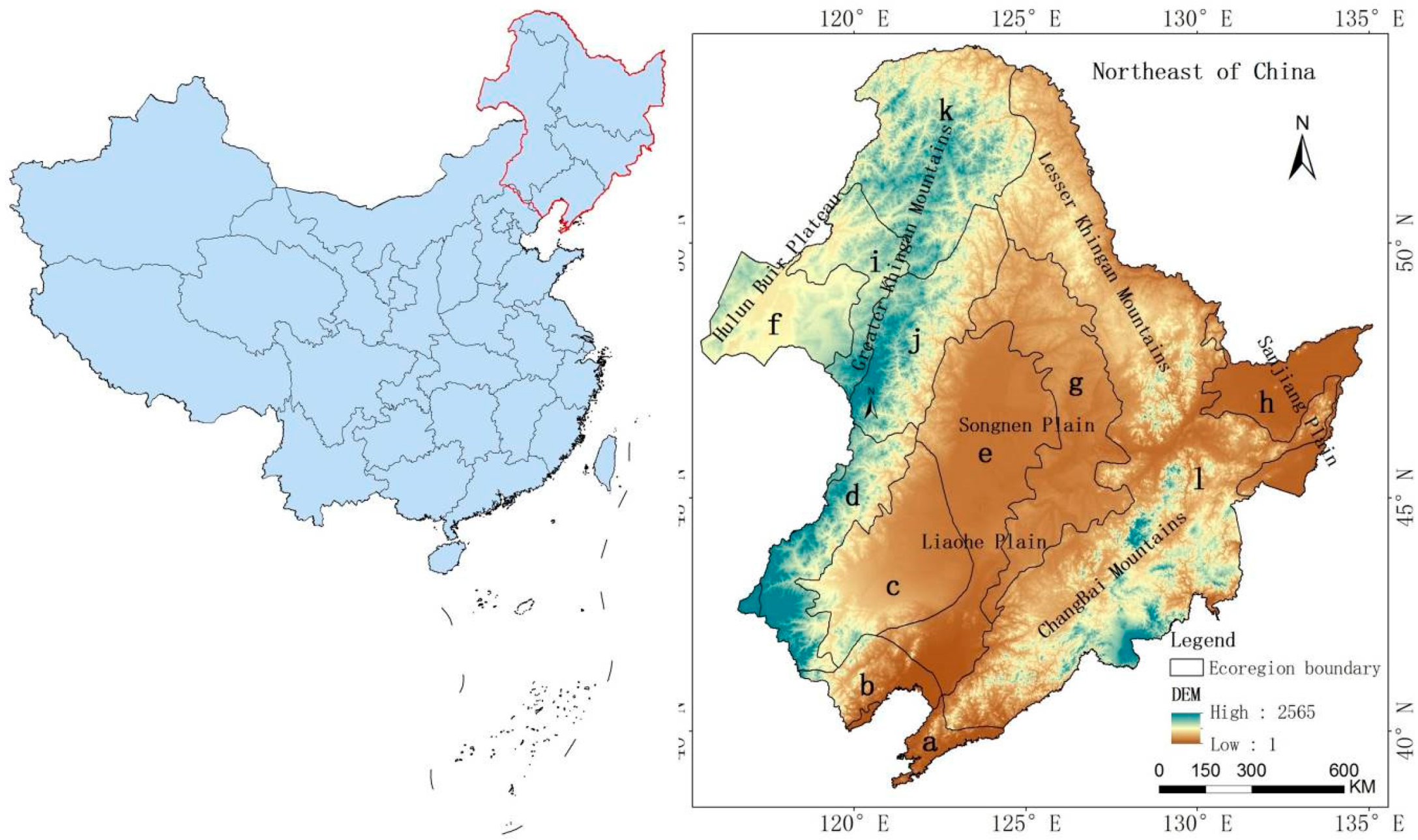
2.1. Study Area

The Northeast China (NEC) region of interest (ROI) is located from 115°32′ to 135°09′E and from 38°42′ to 53°35′N, covers an area of 1.24 million km2 (Figure 1) and exhibits extensive natural diversity with respect to climate, vegetation, geology and soil. The topography of the NEC ROI is characterized by central plains surrounded by mountain ranges. The central plains include the Liao River Plain and the Songnen Plain in the southern and northern parts of the ROI, respectively. The Greater Khingan Mountains, the Lesser Khingan Mountains and the Changbai Mountains surround the plains to the west, northwest and east, respectively. The Sanjiang Plain is located in the northeast corner of the NEC ROI. The Liao River, Songnen and Sanjiang Plains form the Northeast Plain [30]. The entire study area includes the following 12 main ecological regions: (a) low-hill larch and broadleaf forest and artificial vegetation in eastern Liaoning and Shandong (LLS); (b) larch and broadleaf forest areas in the mountains of North China (LMN); (c) a grassland area in the Xiliaohe Plain (GXP); (d) a grassland area at the southern end of the Greater Khingan Mountains (GGM); (e) a forest grassland area in the center of the Songliao Plain (FXP); (f) a plain grassland area in the Hulunbuir plain (PHP); (g) a coniferous and broadleaf mixed forest area in the eastern piedmont tableland of the Songliao Plain (CSP); (h) wetlands of the Sanjiang Plain (WSP); (i) a forest grassland area on the western side of the northern segment of the Greater Khingan Mountains (FGM); (j) a mountain grassland forest area in the middle segment of the Greater Khingan Mountains (MGM); (k) a coniferous forest area in the Changbai Mountains in the Lesser Khingan Mountains (CLM); and (l) a larch and coniferous forest area in the northern segment of the Greater Khingan Mountains (LGM) [31].

2.2. GIMMS NDVI3g Dataset

This study used the Global Inventory Modeling and Mapping Studies (GIMMS) Normalized Difference Vegetation Index 3rd generation (NDVI3g) dataset, which is the latest version of the GIMMS NDVI produced by the NASA Global Inventory Modeling and Mapping Studies group. The dataset is available from July 1981 to December 2013, with 15-day composite and 8 km spatial resolution images. This dataset consists of better quality data at high latitudes than earlier versions and has better calibration capabilities because it uses Sea-Viewing Wide-Field-of-View Sensor (SeaWifs) data instead of SPOT-VGT data [32,33]. The GIMMS 3g dataset was obtained directly from the NASA Ames Ecological Forecasting Lab [34].

2.3. Climate Data

The meteorological data presented in this study include daily temperature and precipitation data from 1982 to 2013 that were acquired from the Chinese Meteorological Science Data Sharing Service Network [35]. These data were recorded at 99 meteorological and climatological stations distributed throughout Northeast China. All meteorological data were examined and verified by China’s Meteorological Information Center. This study calculated the mean temperature and cumulative precipitation every month, spring (3–5 months), summer (6–8 months) autumn (9–11 months), winter (12–2 (next year) months) and year in Northeast China for all the sites from 1982 to 2013. To analyze the correlation between the LSP and climate data, we used the kriging interpolation method to interpolate the temperature and precipitation data from the stations into 8 km × 8 km grids to match the GIMMS 3g data. The grid data have the same spatial and temporal resolution and projection system as the GIMMS3g data.

2.4. Phenology Metrics

Products of long-term series datasets, such as the GIMMS 15-day maximum synthesis, MODIS 8-day and 16-day maximum synthesis and SPOT VGT 10-day maximum synthesis, are commonly used in the maximum synthetic treatment process [36]. However, due to the effects of cloud, atmosphere, sensor and surface bidirectional reflectance [12,37], the original synthesized NDVI time series will contain some singular values. Performance limitations are perceptible when these data are used, especially in a single cell, as the main focus is on dips or needlepoint humps in the NDVI time series. Singular values will affect the precision of the dataset and require further processing to reduce the influences of noise and provide more effective time series datasets.
Scholars have proposed several time series reconstruction algorithms, such as the best index of slope extraction method [38], the average iterative filtering method [39], the Fourier transform method [40], the Savitzky-Golay filtering method [6,41,42,43], the asymmetric Gaussian fitting method [42,44], the wavelet analysis method [45] and linear interpolation within the time window [46]. Accurate remotely sensed time series data require a noise smoothing process to remove leakage points and vacancy points within the series. The TIMESAT software [44,47] is a widely used program [48,49,50,51,52,53] that uses TIMESAT with Savitzky-Golay filtering (S-G), asymmetric Gaussian curves (AG), or double logistic functions (DL) to fit NDVI data and reduce drop-outs or gaps in data series covering a long period [47,54,55].
Zhao studied the differences between the asymmetric Gaussian, double logistic, and adaptive Savitzky-Golay fitting methods and found very small differences in the phenology results obtained from the three methods (Root Mean Square Errors (RMSE) of 0.0416, 0.0429 and 0.0370 for the AG, DL and S-G methods, respectively). In addition, this study presents correlation coefficients between the extracted starting date and the observed starting date from 1999 to 2009 (0.82 (p < 0.01), 0.79 (p < 0.01) and 0.66 (p < 0.01) for the AG, DL, and S-G fitting methods, respectively) [56]. In this paper, we chose Savitzky-Golay filtering.
We employed TIMESAT to generate smooth time series NDVI data and adopted an adaptation strength of 2.0, no spike filtering, a seasonal parameter of 0.5, a Savitzky-Golay window size of 2 and an amplitude of 30% at the beginning and end of the season to calculate the phenology parameters. We calculated the SOS and EOS for each year and obtained the LOS as the difference between the SOS and EOS at each grid point [16].

3. Results

3.1. The Mean Spatial Distribution of Land Surface Phenology

To analyze the spatial distribution of the land surface phenology in Northeast China, this study calculated the average values of the SOS and EOS in Northeast China over the past 32 years (1982–2013) (Figure 2). The SOS values in Northeast China are divided into two groups by the 140th day (mid-May) (Figure 2a). The SOS values in the plain areas, most of which occurred between the 140th and 155th day, were significantly later than those of the vegetation in the mountainous areas. In addition, vegetation with a late SOS was mainly located in the Songnen, Sanjiang and Liaohe Plains, which are the main grain producing areas in Northeast China and primarily produce maize, soybeans and rice. These crops are greatly affected by sowing time and have SOS dates that are significantly later than those of other vegetation types. The vegetation in the Changbai Mountains, Lesser Khingan Mountains and Greater Khingan Mountains had relatively early SOS dates between the 115th and 140th day. The vegetation in the southwestern Changbai Mountains near the coast had relatively early SOS dates, whereas the vegetation in the northernmost Greater Khingan Mountains had relatively late SOS dates.
The spatial distribution of the EOS is different from that of the SOS. The EOS dates of the crops were not significantly different from those of the other vegetation types, whereas the SOS dates of crops were significantly affected by human factors (e.g., sowing time). Therefore, the EOS gradually became later from north to south, and the latest EOS occurred in the Changbai Mountains. The Changbai Mountains are located at relatively low latitudes, are affected by monsoons, and have more pronounced hydrothermal conditions than other regions; therefore, the EOS dates in the Changbai Mountains were later than those in the other areas.

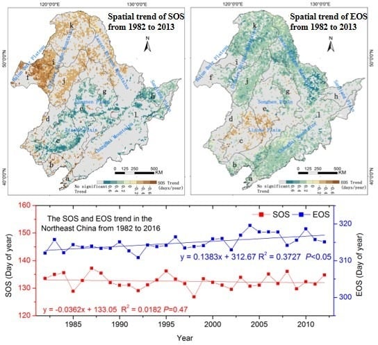
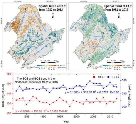
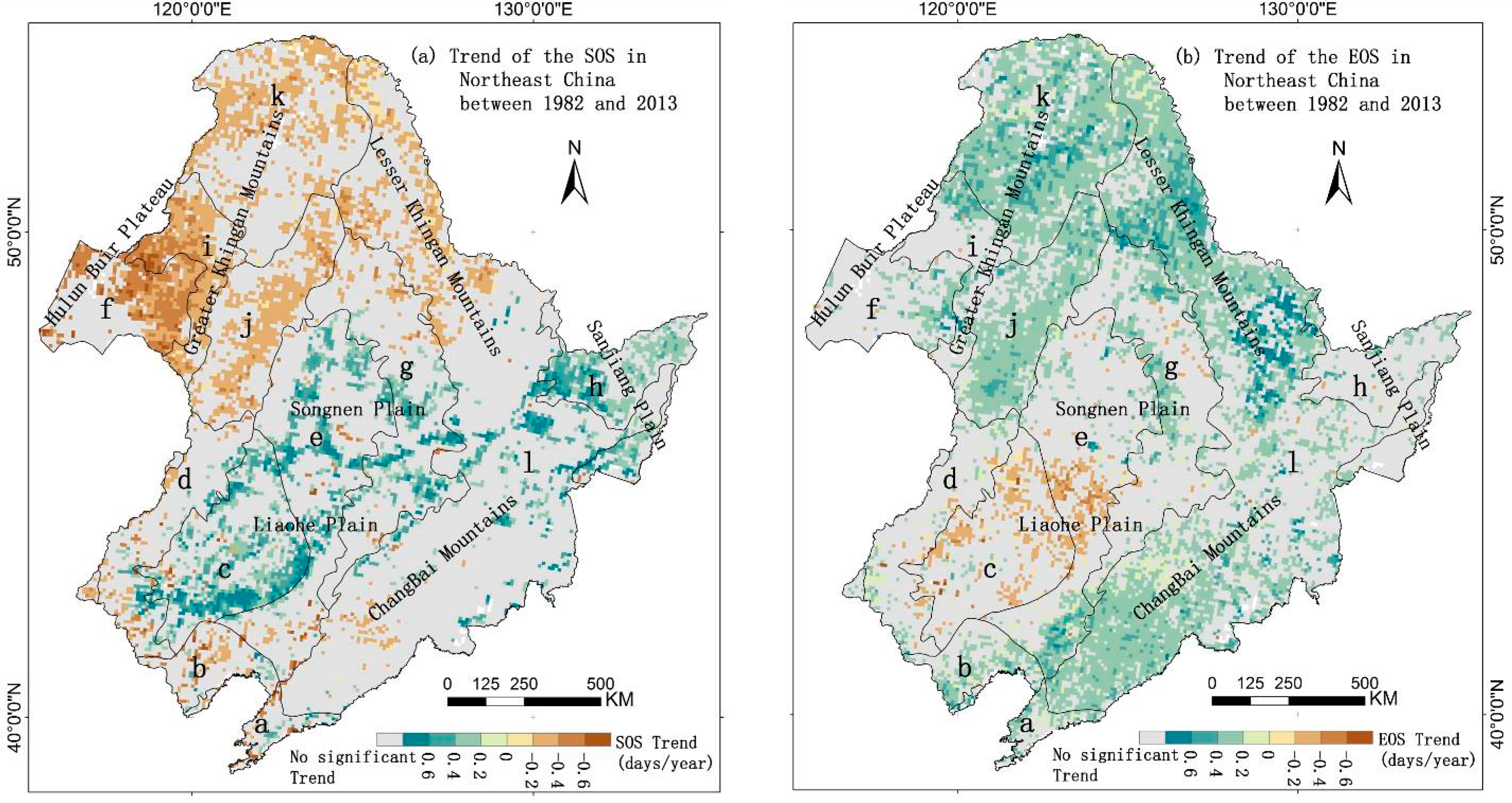
3.2. Spatial Phenology Trends

The linear trends of the SOS and EOS were calculated at the 95% confidence level (Figure 3a,b). Over the past 32 years, 30% of the pixels in the study area showed significant changes in the SOS (Figure 3a). The SOS of the mountain vegetation in the northern study area advanced significantly (p < 0.05), with 53.34% of the pixels showing significant changes. Most of the vegetation types with significantly advanced SOS dates grew in the deciduous coniferous forests in the northern segment of the Greater Khingan Mountains, the forest grassland area on the western side of the northern segment of the Greater Khingan Mountains, the grassland area in the Hulunbuir Plain, and the grassland and forest areas in the middle segments of the Greater Khingan Mountains and Lesser Khingan Mountains. The SOS dates for the vegetation types in the plains in the center of the study area, including the forest and grassland area in the center of the Songliao Plain and the grassland area south of the Xiliaohe Plain, were significantly later (p < 0.05). The mean SOS date in the Changbai Mountains was the earliest (Figure 2), and the variation of the SOS in the Changbai Mountains was insignificant. For the EOS, 39.11% of the pixels exhibited significant delays (p < 0.05), which accounted for 91.86% of the pixels that exhibited a significant variation.
The EOS exhibited an advancing trend in a small area of the Liaohe Plain and a relatively significant advancing trend (p < 0.05) in the forest grassland area in the center of the Songliao Plain and the grassland area of the Xiliaohe Plain. Most of the vegetation types with significantly delayed EOS dates were located in the deciduous coniferous forests in the northern segment of the Greater Khingan Mountains and the mountain grassland forest area in the middle segment of the Greater Khingan Mountains and Lesser Khingan Mountains (Figure 3b). The EOS dates in the southern area of the Changbai Mountains also exhibited an advancing trend; however, the variations of the EOS in the northern foothills of the Changbai Mountains were insignificant at the 95% confidence level.
The number of pixels that show advanced SOS dates is equivalent to the number of pixels that show delayed SOS dates. However, most of the pixels show a significant delay in the EOS. The EOS dates of the vegetation in the areas where the SOS exhibited an advancing trend were all delayed. Therefore, the phenology in Northeast China is affected more by the EOS than by the SOS.

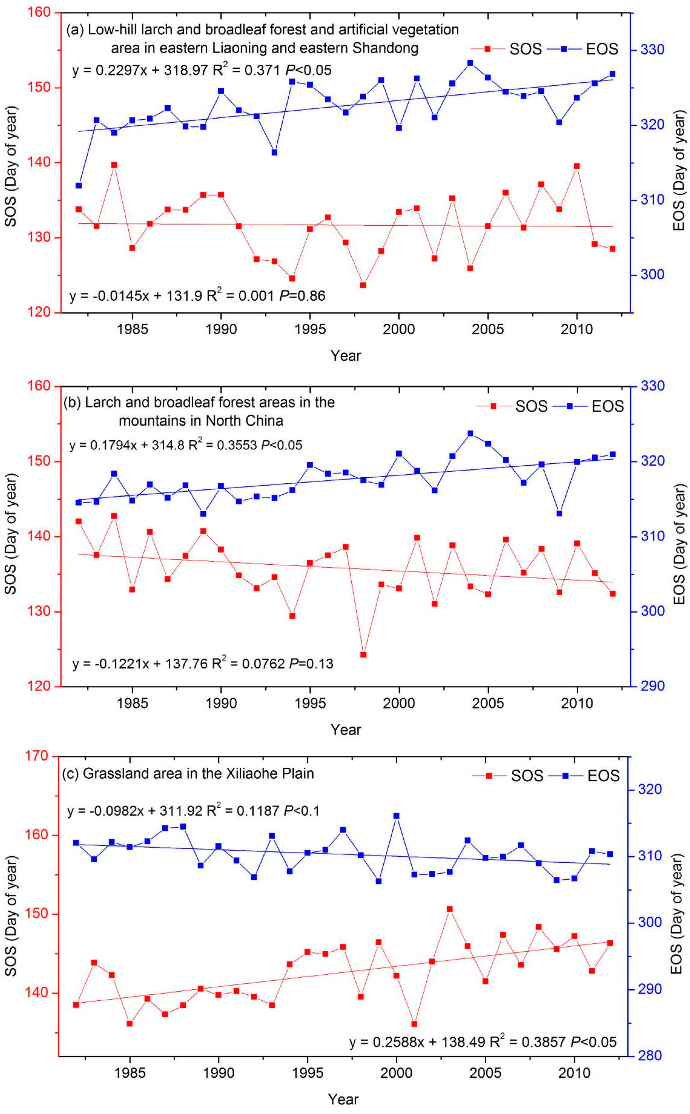
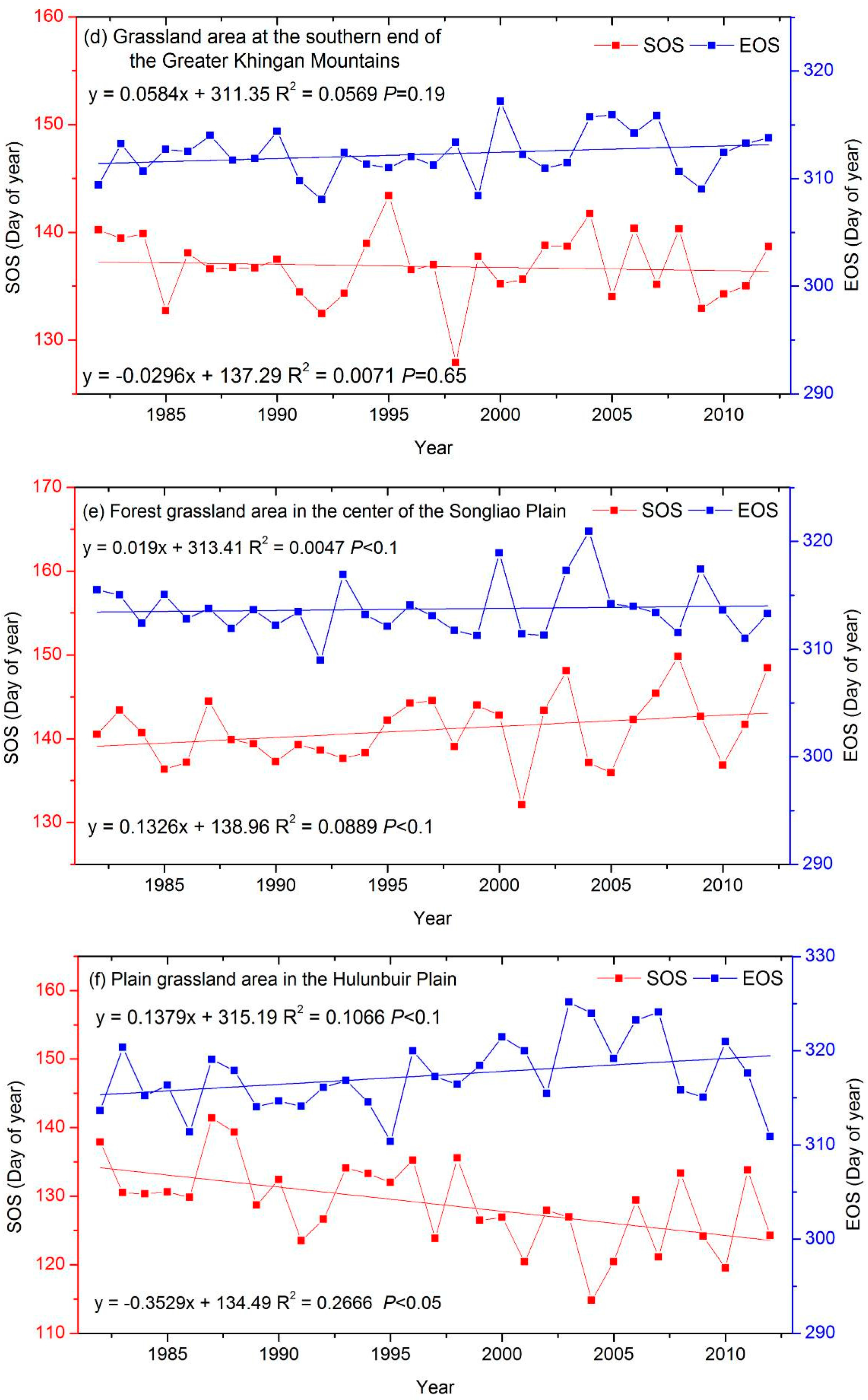
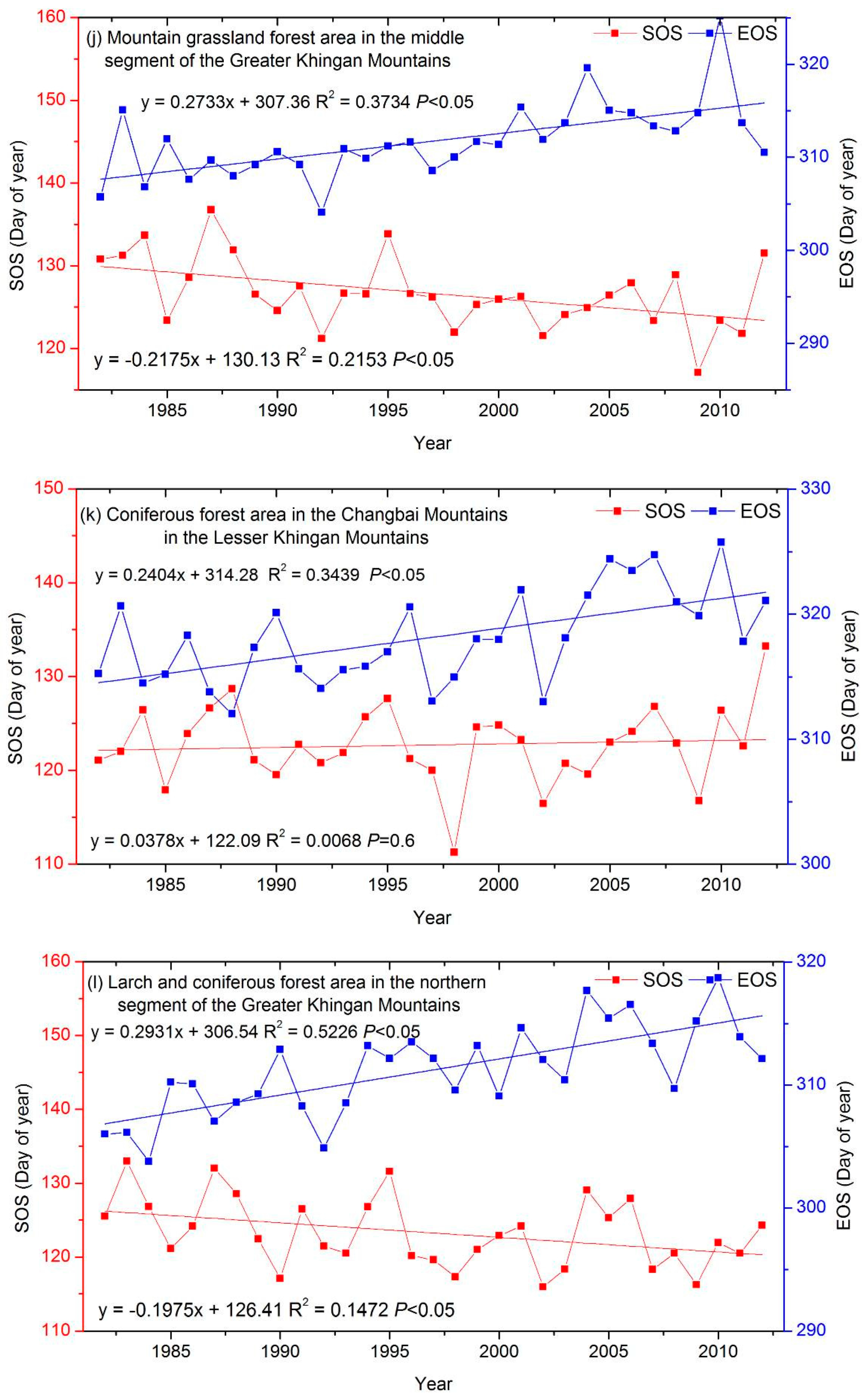
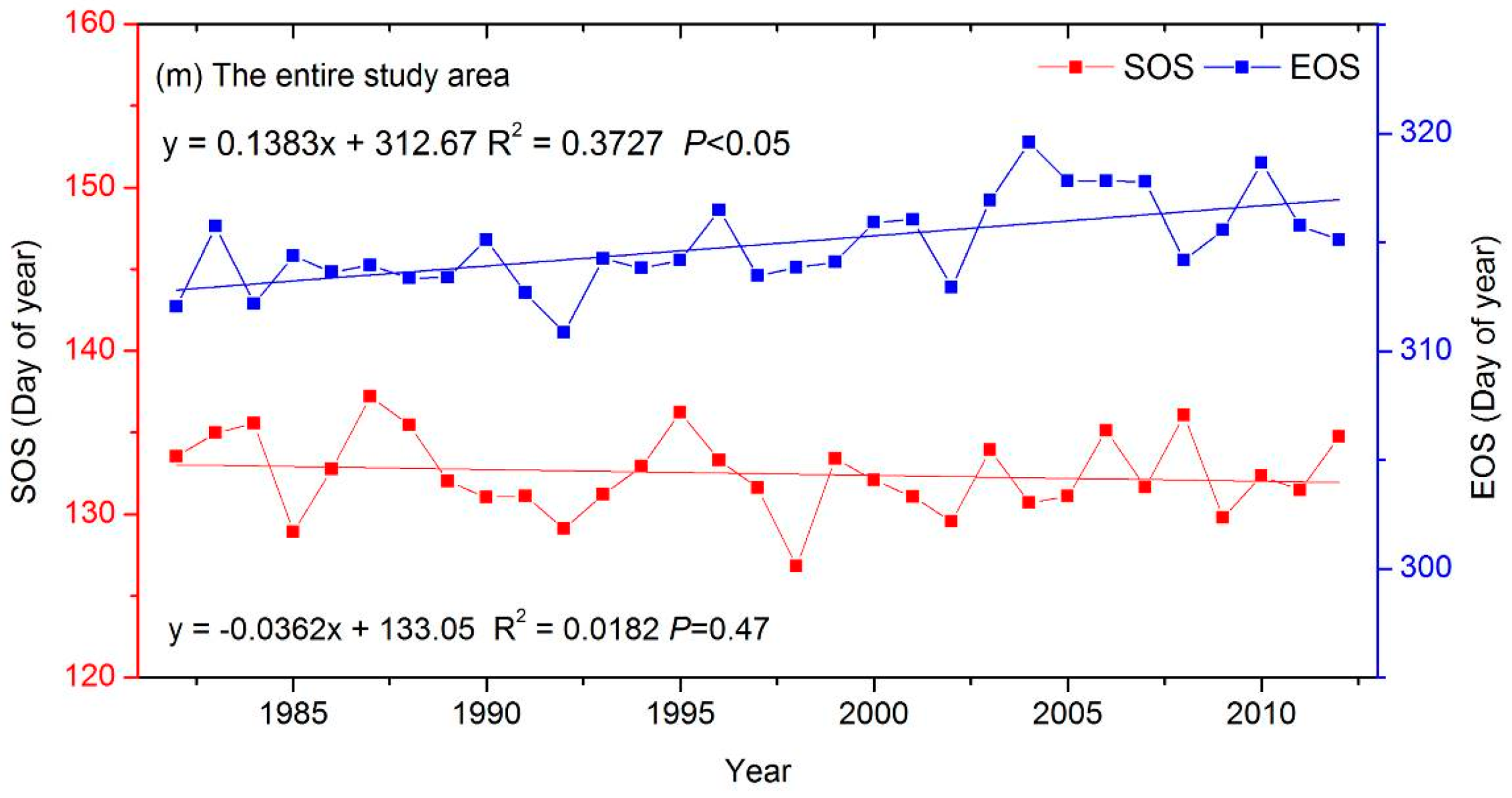
3.3. The Interannual Variability and Trends of LSP Metrics in Different Ecological Areas

This study analyzed the long-term variations of the land surface phenology in 12 ecological regions in the study area and across the entire study area (Figure 1).
Large differences can be observed in the variations of the SOS and EOS in the different ecological areas (Figure 4 and Table 1). The SOS of the vegetation advanced significantly in the larch and coniferous forest area in the northern segment of the Greater Khingan Mountains (Figure 4l; −0.2 days/year, p < 0.05), the mountain grassland forest area in the middle segment of the Greater Khingan Mountains (Figure 4j; −0.22 days/year, p < 0.05), the forest grassland area on the western side of the northern segment of the Greater Khingan Mountains (Figure 4i; −0.31 days/year, p < 0.05) and the plain grassland area in the Hulunbuir Plain (Figure 4f; −0.35 days/year, p < 0.05). The SOS in the plains grassland area of the Xiliaohe Plain (Figure 4c; 0.26 days/year, p < 0.05) and the wetland area of the Sanjiang Plain (Figure 4h; 0.25 days/year, p < 0.05) exhibited significant delays.
The EOS dates of the vegetation in all of the ecological areas, except for the grassland area in the Xiliaohe Plain, which exhibited an advancing trend of 0.1 days/year (p < 0.1), exhibited significant delays. Figure 4l shows the delays of the EOS for the larch and coniferous forest area in the northern segment of the Greater Khingan Mountains (0.29 days/year, p < 0.05), and Figure 4j shows the delays of the EOS for the grassland forest area in the middle segment of the Greater Khingan Mountains (0.27 days/year, p < 0.05). Figure 4k shows the delays of the EOS for the coniferous forest area in the Changbai Mountains in the Lesser Khingan Mountains (0.24 days/year, p < 0.05), and Figure 4a shows the delays of the EOS for the low-hill larch and broadleaf forest area and the artificial vegetation area in eastern Liaoning and eastern Shandong (0.23 days/year, p < 0.05). Figure 4b shows the delays of the EOS for the mountainous larch and broadleaf forest area in northern China (0.18 days/year, p < 0.05), and Figure 4i shows the delays of the EOS for the forest grassland area on the western side of the northern segment of the Greater Khingan Mountains (0.16 days/year, p < 0.05).
The SOS in the Hulunbuir Plain exhibited a significant advance of 10.8 days; however, the EOS was delayed by 4.3 days. The SOS dates for the three ecological areas in the Greater Khingan Mountains all exhibited relatively significant advances, whereas the EOS dates all exhibited relatively significant delays.
For the entire study area (Figure 4m), the SOS exhibited a clear advancing trend of 0.02 days/year; however, the variation of the SOS was insignificant (p = 0.47). The EOS of the vegetation across the entire study area exhibited a significant delay of 0.128 days/year (p < 0.05). Therefore, the phenological changes throughout Northeast China were reflected by changes in the EOS, which is consistent with the pixel-scale spatial distribution of the EOS shown in Figure 3b.

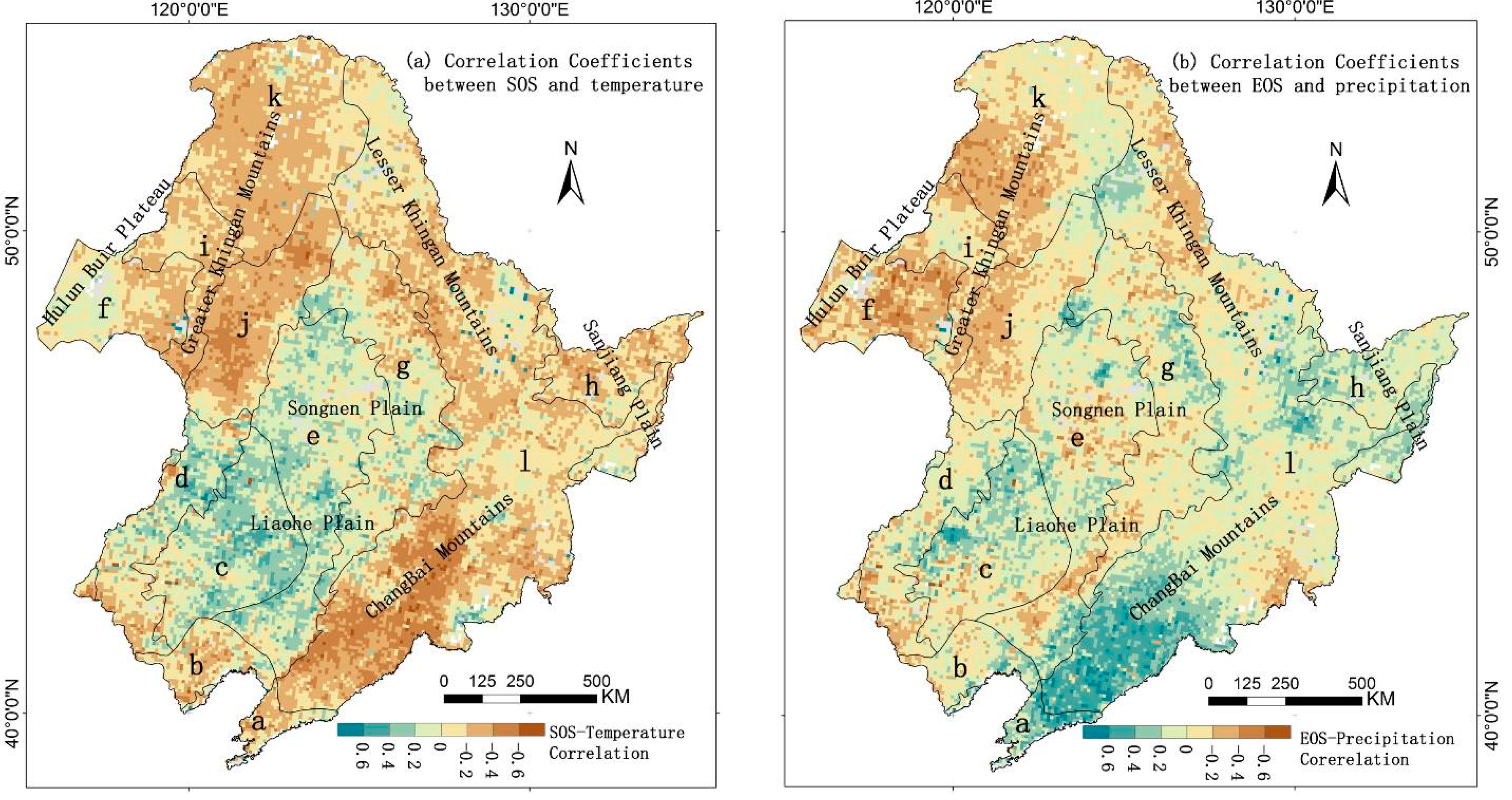
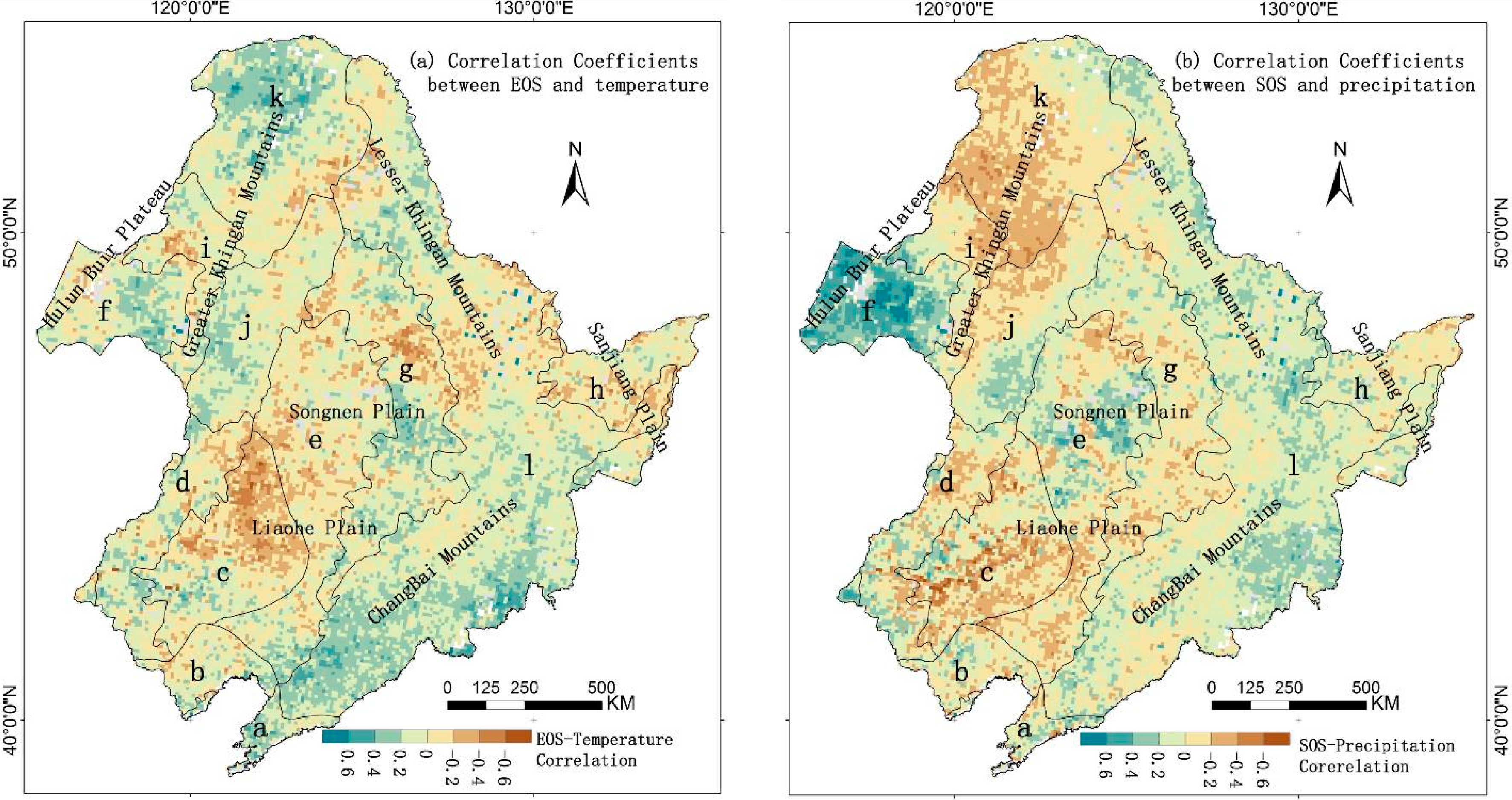
3.4. Direct Effects of Local Climate Factors on LSP

To further analyze the effects of temperature and precipitation on the land surface phenology changes in Northeast China, this study analyzed the correlations between the SOS and EOS and the monthly, seasonal and annual total precipitation and mean temperature from 1982 to 2013.
Figure 5a shows that the SOS dates in the Changbai Mountains, Lesser Khingan Mountains and Greater Khingan Mountains were negatively correlated with temperature. Thus, increasing temperature promoted the advancement of the SOS, particularly in the forest areas. However, the SOS dates in the Songnen Plain were insignificantly or negatively correlated with temperature. The analysis of the correlations between different seasonal and annual mean temperatures and the SOS showed that the SOS was most significantly correlated with the spring temperature, followed by the summer temperature and the annual mean temperature. The pixels that were significantly and negatively correlated with the spring, summer and annual mean temperatures accounted for 35%, 16% and 10% of the total pixels, respectively, indicating that the spring temperature had the largest impact on the SOS and fall and winter temperatures had relatively small impacts on the SOS. The SOS in Northeast China ranged from the 115th day (April) to the 155th day (June), and the SOS dates were relatively significantly and negatively correlated with temperature during the same period (an increase in temperature resulted in SOS advancement).
The spatial distribution of the correlation coefficients between the SOS and precipitation (Figure 5b) shows that the SOS in the grassland area in the Hulunbuir Plain was negatively correlated with precipitation and that the SOS at the northern end of the Greater Khingan Mountains was positively correlated with precipitation. These results indicate that precipitation can advance or delay the SOS. The advancement of the SOS by precipitation was prominent in the grassland areas. However, precipitation was not the dominant factor that determined the SOS of the vegetation in the forests. The results of the significance test between the SOS and precipitation (Table 2) show that the highest proportion of pixels that were significantly and positively correlated with precipitation occurred in the spring (6% of the total pixels). In addition, 4% of the pixels were significantly and negatively correlated with precipitation. These results indicate that spring precipitation was significantly correlated with vegetation growth. In addition, the highest proportion of pixels that were significantly and negatively correlated with precipitation was 2% during the winter, which indicates that the effect of precipitation on the SOS was somewhat delayed and that abundant winter precipitation would advance the SOS.
The spatial distributions of the correlation coefficients (Figure 6) between the EOS and temperature and between the EOS and precipitation show that the EOS dates in the plain areas were mainly negatively correlated with the annual mean temperature and that the EOS dates in the other areas were positively correlated with the annual mean temperature. The results of the significance test (Table 3) show that the fall temperature had the largest impact on the EOS (16% of the pixels were significantly and positively correlated with temperature), indicating that an increase in the fall temperature would delay the EOS. The spatial distribution of the correlation coefficients between the EOS and precipitation (Figure 6b) shows that the EOS dates in the southwestern Changbai Mountains were positively correlated with precipitation and that the EOS dates in the Greater Khingan Mountains were negatively correlated with precipitation. The results of the significance test between the EOS and precipitation (Table 3) show that spring, fall, winter and annual precipitation all affected the EOS. In addition, the number of positively correlated pixels was significantly higher than the number of negatively correlated pixels, and a relatively small number of pixels were significantly and negatively correlated.

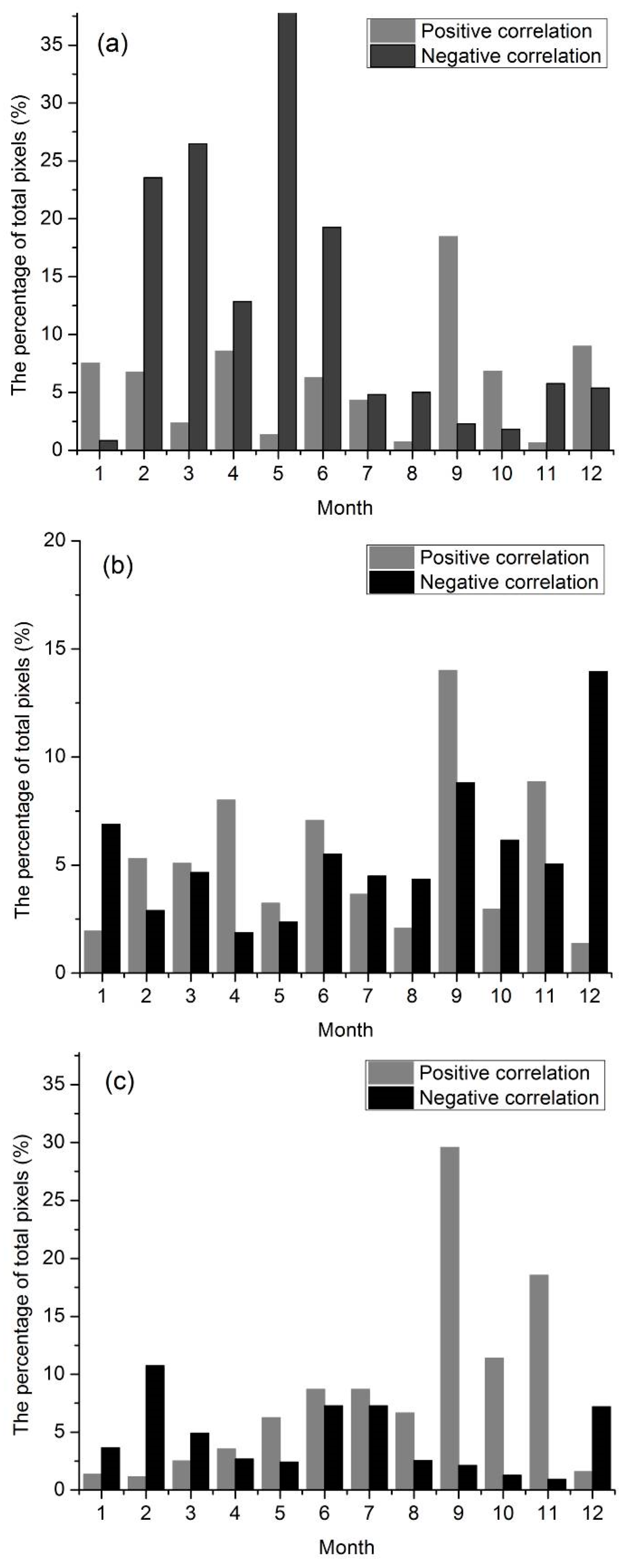
3.5. Lag Effect of Climate Change on Land Surface Phenology

To analyze the degree to which the variations in the monthly temperature and precipitation affect the SOS and EOS, this study analyzed the correlations between the SOS and temperature and between the SOS and precipitation from July of the previous year to June of the same year and the correlations between the EOS and temperature and between the EOS and precipitation from January to December of the same year (Figure 7). The SOS dates were relatively significantly and negatively correlated with temperature from February to June of the same year, and temperature had a clear advancing effect on the SOS throughout Northeast China (temperature increases resulted in the advancement of the SOS and vice versa) (Figure 7a). The temperature during the first few months of the growing season had an insignificant impact on the SOS. The SOS dates were insignificantly correlated with precipitation within the same year and significantly correlated with precipitation during the first few months of the year. The precipitation from September to December of the previous year advanced the SOS of the next year, and increases in precipitation advanced the SOS.
The proportion of pixels that showed positive correlations between temperature and the EOS gradually increased from April to November within the same year, and the proportion of pixels that showed a positive correlation between temperature and the EOS from September to November within the same year was the most significant. This result indicates that temperature had a clear advancing effect on the EOS because increasing temperature caused a delay in the EOS and vice versa (Figure 7c). The precipitation from November of the previous year to August of the following year had a clear advancing effect on the EOS of the following year, and the precipitation from September to October had a clear delaying effect on the EOS of the same year (Figure 7d). Therefore, precipitation caused a delay in the EOS. However, the effects of precipitation on the EOS were insignificant; thus, precipitation was not the dominant factor responsible for delaying the EOS.

4. Discussion

4.1. Variations of Land Surface Phenology

The LSP results are different because different data sources and different models were used. When the same model was used with a different threshold, the results were different, and the accuracy of the inversion results can be improved by combining them with ground observation data.
The results of this study indicate that the average SOS is primarily between Julian days 110 and 150, which is consistent with previous studies [29,57,58,59]. Luo et al. showed that the SOS of deciduous broadleaf forest regions in northern China is between Julian days 115 and 130 [60]. In addition, this study showed that the SOS of deciduous broadleaf forests in northern China mainly occurred between Julian days 115 and 140, and the ground observation data showed that the SOS of the deciduous broad-leaved forest mainly occurred between Julian days 111 and 140. The SOS observed in our study was similar to the SOS observed by Luo et al. in the field. The EOS in this study is primarily between Julian days 270 and 320. The study of Liu et al. shows that the mean EOS values for the four methods are mainly distributed from 270 to 310 [61]. The results of Yang et al. show that vegetation in temperate China becomes dormant in the autumn between Julian days 228 and 359 [62]. The EOS in this study is higher than that identified by Liu [61]. In addition, we obtained phenology data from 14 field sites with more than 180 species of plants in Northeast China from 1982 to 1988. The results demonstrate that these SOS plants mainly grow between 110 and 150 DOY. The EOS was mainly between 260 and 320 DOY. These results coincide with the results of this study, which shows that the extracted phenology has a certain reference value and reliability.
Liu et al. used four different methods to estimate the EOS and compared their results. Overall, the results based on the HANTS-Mr, Polyfit-Mr, and piecewise logistic methods showed similar patterns, and the results based on double logistics indicated much earlier EOS dates [61]. In this paper, it was estimated that the EOS was delayed by 0.14 days/year. Liu et al. used the mean results from four methods and showed that the EOS changed by 0.12 ± 0.01 days/year for temperate vegetation in China [61]. The results of Yang et al. reported changes in the EOS, with an average delay of 0.13 days per year over temperate China from 1982 to 2010 [62]. Xia & Yan showed an EOS change of 0.05 days/year from 1909 to 2012 based on station records [63]. Our estimated EOS values were 0.02, 0.01 and 0.08 days/year greater than those of Liu [61], Yang [62], and Xia & Yan [63], respectively. Our study area is located at a higher latitude than previous study areas [61,62,63]. In addition, the vegetation at high latitudes is more susceptible to climate change [16,64,65,66,67,68], which is supported by our results. Shrestha et al. studied the climatic and phenological changes for 13 ecoregions of the Himalayas during 1982 and 2006 [69]. The result show that the average SOS appeared to advance by 4.7 or 0.19 days/year, but no change in the EOS [69] was observed. However, some differences between Shrestha’s results and the results of our study were observed for the entire study areas.
Different cover types significantly influence the SOS and EOS trends. The main types of land cover are grasses in the plain grassland area in the Hulunbuir Plain (PHP), forest in the forest grassland area on the western side of the northern segment of the Greater Khingan Mountains (FGM), mountain grassland forest in the middle segment of the Greater Khingan Mountains (MGM) and larch and coniferous forest in the northern segment of the Greater Khingan Mountains (LGM) ecoregions. The SOS have significantly advanced by 0.35 days/year (p < 0.01), 0.31 days/year (p < 0.01), 0.22 days/year (p < 0.01), and 0.2 days/year (p < 0.05) in these ecoregions (PHP, FGM, MGM and LGM). Simultaneously, the EOS values of the PHP, FGM, MGM and LGM ecoregions were significantly delayed by 0.14 days/year (p < 0.1), 0.16 days/year (p < 0.05), 0.27 days/year (p < 0.01), and 0.29 days/year (p < 0.01). Both grasses and forests are natural vegetation, which requires little management and is less disturbed by humans. These areas reflect the impacts of climate change better than the other areas. The main land cover types are cultivated land in the grassland area in the Xiliaohe Plain (GXP), forest grassland in the center of the Songliao Plain (FXP), coniferous and broadleaf mixed forest in the eastern piedmont tableland of the Songliao Plain (CSP) and wetlands in the Sanjiang Plain (WSP). The SOS in these ecoregions (GXP, FXP, CSP and WSP) is delayed by 0.26 days/year (p < 0.01), 0.13 days/year (p < 0.1), 0.13 days/year (p < 0.1), and 0.25 days/year (p < 0.01), respectively. The land cover has changed over the past 32 years in these three ecoregions mainly composed of agriculture. Shrestha’s results show that the SOS significantly advanced in the forest area at the ecoregion scale, which is similar to the findings of our study [69]. In addition, another study shows that the area of farmland steadily increased from the late 1970s to 2000 [70], with the conversion of some natural vegetation (such as forest and grass) land to cultivated land. The SOS of agricultural land is later than that of natural vegetation, and the EOS of agriculture is earlier than that of natural vegetation. Therefore, land cover changes will result in the LSP trends of vegetation. Simultaneously, farmers have switched to new crop varieties, such as faster-maturing varieties, which may contribute to the early SOS dates. The types of crops grown changed in the central and western regions of the Songnen Plain and in part of the Sanjiang Plain [71,72]. For example, the area of rice planting increased, and the area of spring wheat planting significantly decreased. Simultaneously, the crop breeding and cultivation mode changed dramatically in Northeast China [73,74]. For example, famers selected maize with a long growth period, rice with improved yield, and soybean and spring wheat with shorter growth periods (between sowing and harvesting time) [75].

4.2. Relationships between LSP Metrics and Climatic Factors

The results of this study show that the spring temperature has the greatest impact on the SOS because it increases as the SOS advances. This finding agrees with the findings of Yu and Li, who indicated that the SOS was mainly driven by temperature variations [29,76,77]. Yu et al. extracted forest phenology parameters using MODIS EVI from 2000 to 2009 [60]. The results of Yu et al. show that the SOS was mainly affected by temperature in the spring. The EOS of grasslands is affected by temperature and precipitation in August [29], and the SOS primarily depends on temperature during the other months [29]. The research results of Li show that the temperature has the biggest influence on the SOS from February to April [78]. This study shows that precipitation has a lagging effect on the SOS, the amounts of precipitation in different months affect the EOS, the distributions of different vegetation types depend on precipitation, and the largest and smallest impacts are observed for grasslands and forests, respectively. Piao et al. showed that changes in China’s temperate precipitation affect the vegetation growth period. The degree of influence is different for different types of vegetation [24]. This study shows that the SOS presents an early trend, with 0.15 days per year, and the EOS presents a delayed trend, with 0.16 days per year, in the study area from 1982 to 2005. Li and other researchers have shown similar trends [76]. In 2000–2009, Yu et al. showed that both the SOS and EOS showed delayed trends, whereas in this study, no significant trends for the SOS were observed after 2000, and the EOS delay slowed down [29].

4.3. Uncertainty

The time period investigated in this study (1982–2013) was relatively long and exhibited changes in the vegetation types in Northeast China. In the late 1980s, a catastrophic conflagration occurred in the Greater Khingan Mountains, and the vegetation underwent succession and recovery processes. The three major plains in Northeast China mainly consist of cultivated land and are significantly affected by human factors that result in uncertain land surface phenology. However, in certain areas, such as in the Changbai Mountains, nature reserves and old-growth forests exist that reflect the growth processes of natural vegetation over the past 32 years. When good natural conditions have been maintained, the impacts of climate change are better reflected. Pixel scale analyses can be used to avoid uncertainties that are introduced by regional scale analyses and can reflect the impacts of regional climate change. Analyzing changes in land surface phenology in different ecological areas can also reflect the hydrothermal effects in different areas, identify typical areas with increased sensitivity, and provide a basis for subsequent high-precision, multi-angle analytical studies on the variations and influencing factors of land surface phenology. Because a certain interval in the time series data exists, the result was different when we used a different model or the same model at different thresholds to estimate the phenological parameters. In this study, we investigate the phenological vegetation variation characteristics over the past three decades based on long time series remote sensing data with a spatial resolution of 8 km. Some spatial resolution will be lost when using remote sensing data with a high temporal resolution. Mixed pixels are observed in the data with a spatial resolution of 8 km. Each pixel value is the mean value for all land cover types over an area of 64 square kilometers. These values result in uncertainty in our estimation results. When using the phenology data from the field observations of tree species, a certain error occurs when the data are used to verify the results obtained from remote sensing. In the future, different scales of remote sensing data can be considered for cross validation and to improve the accuracy of phenological estimations.

5. Conclusions

In this study, the land surface phenology parameters of Northeast China were extracted from the GIMMS NDVI 3g dataset that was collected from 1982 to 2013 to analyze the characteristics of land surface phenology changes at several scales and the effects of temperature and precipitation on land surface phenology. The results of this study provide a good reference for studying the regional responses to global climate change.
Spatially, the SOS was gradually delayed and the EOS gradually advanced from south to north in the study area. The SOS dates in the plain areas were significantly later than those in the mountainous areas, and a significant difference was observed in the spatial distribution of the phenology between the forest areas and grassland areas. In most areas, the SOS dates of the mountain vegetation significantly advanced, and the EOS dates of the mountain vegetation were significantly delayed. Over the past 32 years, the SOS throughout the entire study area exhibited an insignificant advancing trend, and the EOS exhibited a significant decreasing trend. Different ecological areas exhibited different variations. The variations of the three ecological areas in the Greater Khingan Mountains were the most prominent. The SOS dates in the forest grassland area on the western side of the northern segment of the Greater Khingan Mountains advanced by −0.31 days/year (p < 0.05), while the SOS in the mountain grassland forest area in the middle segment of the Greater Khingan Mountains advanced by −0.22 days/year (p < 0.05). In addition, the SOS in the larch and coniferous forest area in the northern segment of the Greater Khingan Mountains advanced by −0.20 days/year (p < 0.05).
The correlation between the land surface phenology and climate shows that the SOS was negatively correlated with the spring temperature (an increase in the spring temperature caused an advancement in the SOS and vice versa). The EOS was positively correlated with temperature during the summer and fall, with increasing temperatures resulting in a delayed EOS and vice versa. The phenomenon in which a temperature increase promotes the advancement of the SOS was more prominent in the forest areas; however, the SOS dates in the grassland areas were not significantly correlated with temperature. The effects of precipitation on the SOS were somewhat delayed, and the SOS responded to the temperature of the same period more significantly. The effects of temperature on the EOS were somewhat delayed, and the temperature from September to November played an important role in the EOS. Precipitation was not a dominant factor for the delay of the EOS. The effect of precipitation on the EOS was delayed to a relatively small degree. Land surface phenology changes responded strongly to years with extreme climate conditions. Advances in the SOS and delays in the EOS were prominent in the years with relatively high temperatures and abundant precipitation.

Acknowledgments

The authors would like to thank the entire Global Inventory Modeling and Mapping Studies (GIMMS) group for permitting the use of the NDVI3g dataset. We thank Per Jonsson and Lars Eklundh for making their TIMESAT routine available. This study was supported by the National Natural Science Foundation of China (Grant No. 41501449, 41571489 and 41571405), the Science and Technology Development Project of Jilin Province (Grant No. 20150520069JH), China Postdoctoral Science Foundation (Grant No. 2014M561272), Jilin Postdoctoral Science Foundation (Grant No. RB201353), the Fundamental Research Funds for the Central Universities (Grant No. 2412016KJ026 and 14QIVJJ025) and the State Key Laboratory of Resources and Environmental Information System.

Author Contributions

All authors contributed significantly to this manuscript. Specific contributions include data collection (Jianjun Zhao, Yanying Wang, Shan Yu), data analyses (Jianjun Zhao, Xiaoyi Guo, Shan Yu, Wala Du), methodology (Jianjun Zhao, Hongyan Zhang, Zhengxiang Zhang), and manuscript preparation (Jianjun Zhao, Yanying Wang, Zhengxiang Zhang, Hongyan Zhang, Xiaoyi Guo, Shan Yu, Wala Du, Fang Huang).

Conflicts of Interest

The authors declare no conflict of interest.

References

  1. Stöckli, R.; Vidale, P.L. European plant phenology and climate as seen in a 20-year AVHRR land-surface parameter dataset. Int. J. Remote Sens. 2004, 25, 3303–3330. [Google Scholar] [CrossRef]
  2. De Beurs, K.M.; Henebry, G.M. Land surface phenology, climatic variation, and institutional change: Analyzing agricultural land cover change in Kazakhstan. Remote Sens. Environ. 2004, 89, 497–509. [Google Scholar] [CrossRef]
  3. Bhatt, U.S.; Walker, D.A.; Raynolds, M.K.; Bieniek, P.A.; Epstein, H.E.; Comiso, J.C.; Pinzon, J.E.; Tucker, C.J.; Polyakov, I.V. Recent declines in warming and vegetation greening trends over Pan-Arctic tundra. Remote Sens. 2013, 5, 4229–4254. [Google Scholar] [CrossRef]
  4. Badeck, F.-W.; Bondeau, A.; Böttcher, K.; Doktor, D.; Lucht, W.; Schaber, J.; Sitch, S. Responses of spring phenology to climate change. New Phytol. 2004, 162, 295–309. [Google Scholar] [CrossRef]
  5. Cong, N.; Wang, T.; Nan, H.; Ma, Y.; Wang, X.; Myneni, R.B.; Piao, S. Changes in satellite-derived spring vegetation green-up date and its linkage to climate in China from 1982 to 2010: A multimethod analysis. Glob. Chang. Biol. 2013, 19, 881–891. [Google Scholar] [CrossRef] [PubMed]
  6. Heumann, B.W.; Seaquist, J.W.; Eklundh, L.; Jönsson, P. AVHRR derived phenological change in the Sahel and Soudan, Africa, 1982–2005. Remote Sens. Environ. 2007, 108, 385–392. [Google Scholar] [CrossRef]
  7. Justice, C.O.; Townshend, J.R.G.; Holben, B.N.; Tucker, C.J. Analysis of the phenology of global vegetation using meteorological satellite data. Int. J. Remote Sens. 1985, 6, 1271–1318. [Google Scholar] [CrossRef]
  8. Myneni, R.B.; Keeling, C.D.; Tucker, C.J.; Asrar, G.; Nemani, R.R. Increased plant growth in the northern high latitudes from 1981 to 1991. Nature 1997, 386, 698–702. [Google Scholar] [CrossRef]
  9. Lloyd, D. A phenological classification of terrestrial vegetation cover using shortwave vegetation index imagery. Int. J. Remote Sens. 1990, 11, 2269–2279. [Google Scholar] [CrossRef]
  10. Fischer, A. A model for the seasonal variations of vegetation indices in coarse resolution data and its inversion to extract crop parameters. Remote Sens. Environ. 1994, 48, 220–230. [Google Scholar] [CrossRef]
  11. Reed, B.C.; Brown, J.F.; VanderZee, D.; Loveland, T.R.; Merchant, J.W.; Ohlen, D.O. Measuring phenological variability from satellite imagery. J. Veg. Sci. 1994, 5, 703–714. [Google Scholar] [CrossRef]
  12. Zhou, L.; Tucker, C.J.; Kaufmann, R.K.; Slayback, D.; Shabanov, N.V.; Myneni, R.B. Variations in northern vegetation activity inferred from satellite data of vegetation index during 1981 to 1999. J. Geophys. Res. 2001, 106, 20069–20083. [Google Scholar] [CrossRef]
  13. Shabanov, N.V.; Zhou, L.; Knyazikhin, Y.; Myneni, R.B.; Tucker, C.J. Analysis of interannual changes in northern vegetation activity observed in AVHRR data from 1981 to 1994. IEEE Trans. Geosci. Remote Sens. 2002, 40, 115–130. [Google Scholar] [CrossRef]
  14. Zhou, L.; Kaufmann, R.K.; Tian, Y.; Myneni, R.B.; Tucker, C.J. Relation between interannual variations in satellite measures of northern forest greenness and climate between 1982 and 1999. J. Geophys. Res. 2003, 108. [Google Scholar] [CrossRef]
  15. Chen, X.; Hu, B.; Yu, R. Spatial and temporal variation of phenological growing season and climate change impacts in temperate eastern China. Glob. Chang. Biol. 2005, 11, 1118–1130. [Google Scholar] [CrossRef]
  16. Zhao, J.; Zhang, H.; Zhang, Z.; Guo, X.; Li, X.; Chen, C. Spatial and temporal changes in vegetation phenology at middle and high latitudes of the Northern Hemisphere over the past three decades. Remote Sens. 2015, 7, 10973–10995. [Google Scholar] [CrossRef]
  17. Cleland, E.E.; Chuine, I.; Menzel, A.; Mooney, H.A.; Schwartz, M.D. Shifting plant phenology in response to global change. Trends Ecol. Evol. 2007, 22, 357–365. [Google Scholar] [CrossRef] [PubMed]
  18. Julien, Y.; Sobrino, J.A. Global land surface phenology trends from GIMMS database. Int. J. Remote Sens. 2009, 30, 3495–3513. [Google Scholar] [CrossRef]
  19. Jeong, S.-J.; Ho, C.-H.; Gim, H.-J.; Brown, M.E. Phenology shifts at start vs. end of growing season in temperate vegetation over the Northern Hemisphere for the period 1982–2008. Glob. Chang. Biol. 2011, 17, 2385–2399. [Google Scholar] [CrossRef]
  20. White, M.A.; Running, S.W.; Thornton, P.E. The impact of growing-season length variability on carbon assimilation and evapotranspiration over 88 years in the eastern US deciduous forest. Int. J. Biometeorol. 1999, 42, 139–145. [Google Scholar] [CrossRef] [PubMed]
  21. Zhang, X.; Friedl, M.A.; Schaaf, C.B.; Strahler, A.H.; Liu, Z. Monitoring the response of vegetation phenology to precipitation in Africa by coupling MODIS and TRMM instruments. J. Geophys. Res. 2005, 110. [Google Scholar] [CrossRef]
  22. Fitter, A.H.; Fitter, R.S.R.; Harris, I.T.B.; Williamson, M.H. Relationships between first flowering date and temperature in the flora of a locality in central England. Funct. Ecol. 1995, 9, 55–60. [Google Scholar] [CrossRef]
  23. Rötzer, T.; Chmielewski, F.-M. Phenological maps of Europe. Clim. Res. 2001, 18, 249–257. [Google Scholar] [CrossRef]
  24. Piao, S.; Fang, J.; Zhou, L.; Ciais, P.; Zhu, B. Variations in satellite-derived phenology in China’s temperate vegetation. Glob. Chang. Biol. 2006, 12, 672–685. [Google Scholar] [CrossRef]
  25. Zhao, J.; Wang, Y.; Hashimoto, H.; Melton, F.S.; Hiatt, S.H.; Zhang, H.; Nemani, R.R. The variation of land surface phenology from 1982 to 2006 along the Appalachian Trail. IEEE Trans. Geosci. Remote Sens. 2013, 51, 2087–2095. [Google Scholar] [CrossRef]
  26. White, M.A.; Nemani, R.R.; Thornton, P.E.; Running, S.W. Satellite evidence of phenological differences between urbanized and rural areas of the eastern United States deciduous broadleaf forest. Ecosystems 2002, 5, 260–273. [Google Scholar] [CrossRef]
  27. Dash, J.; Jeganathan, C.; Atkinson, P.M. The use of MERIS Terrestrial Chlorophyll Index to study spatio-temporal variation in vegetation phenology over India. Remote Sens. Environ. 2010, 114, 1388–1402. [Google Scholar] [CrossRef]
  28. Busetto, L.; Colombo, R.; Migliavacca, M.; Cremonese, E.; Meroni, M.; Galvagno, M.; Rossini, M.; Siniscalco, C.; Morra di Cella, U.; Pari, E. Remote sensing of larch phenological cycle and analysis of relationships with climate in the Alpine region. Glob. Chang. Biol. 2010, 16, 2504–2517. [Google Scholar] [CrossRef]
  29. Yu, X.; Wang, Q.; Yan, H.; Wang, Y.; Wen, K.; Zhuang, D.; Wang, Q. Forest phenology dynamics and its responses to meteorological variations in Northeast China. Adv. Meteorol. 2014. [Google Scholar] [CrossRef]
  30. Zhang, X.; Wang, W.-C.; Fang, X.; Ye, Y.; Zheng, J. Vegetation of Northeast China during the late seventeenth to early twentieth century as revealed by historical documents. Reg. Environ. Chang. 2011, 11, 869–882. [Google Scholar] [CrossRef]
  31. Zheng, D. China’s Eco-Geographical Region Map; The Commercial Press: Beijing, China, 2008. [Google Scholar]
  32. Zhu, Z.; Bi, J.; Pan, Y.; Ganguly, S.; Anav, A.; Xu, L.; Samanta, A.; Piao, S.; Nemani, R.R.; Myneni, R.B. Global data sets of vegetation leaf area index (LAI) 3g and Fraction of Photosynthetically Active Radiation (FPAR) 3g derived from Global Inventory Modeling and Mapping Studies (GIMMS) Normalized Difference Vegetation Index (NDVI3g) for the period 1981 to 2011. Remote Sens. 2013, 5, 927–948. [Google Scholar]
  33. Dardel, C.; Kergoat, L.; Hiernaux, P.; Mougin, E.; Grippa, M.; Tucker, C.J. Re-greening Sahel: 30 years of remote sensing data and field observations (Mali, Niger). Remote Sens. Environ. 2014, 140, 350–364. [Google Scholar] [CrossRef]
  34. NASA Ames Ecological Forecasting Lab. Available online: http://ecocast.arc.nasa.gov/data/pub/gimms/3g.v0/ (accessed on 15 September 2014).
  35. Chinese Meteorological Science Data Sharing Service Network. Available online: http://www.ncdc.noaa.gov/cag/time-series/global/ (accessed on 1 May 2015).
  36. Holben, B.N. Characteristics of maximum-value composite images from temporal AVHRR data. Int. J. Remote Sens. 2007, 7, 1417–1434. [Google Scholar] [CrossRef]
  37. Tucker, C.J.; Pinzon, J.E.; Brown, M.E.; Slayback, D.A.; Pak, E.W.; Mahoney, R. An extended AVHRR 8-km NDVI dataset compatible with MODIS and SPOT vegetation NDVI data. Int. J. Remote Sens. 2005, 26, 4485–4498. [Google Scholar] [CrossRef]
  38. Viovy, N.; Arino, O.; Belward, A.S. The Best Index Slope Extraction (BISE): A method for reducing noise in NDVI time-series. Int. J. Remote Sens. 1992, 13, 1585–1590. [Google Scholar] [CrossRef]
  39. Jiang, N.; Zhu, W.; Mou, M.; Wang, L.; Zhang, J. A phenology-preserving filtering method to reduce noise in NDVI time series. In Proceedings of the IEEE International Geoscience and Remote Sensing Symposium (IGARSS), Munich, Germany, 22–27 July 2012; pp. 2384–2387.
  40. Song, Y.; Chen, P.; Wan, Y.; Shen, S. Application of hybrid classification method based on fourier transform to time-series NDVI images. In Proceedings of the Congress on Image and Signal Processing, CISP ’08, Sanya, China, 27–30 May 2008; pp. 634–638.
  41. Chen, J.; Jönsson, P.; Tamura, M.; Gu, Z.; Matsushita, B.; Eklundh, L. A simple method for reconstructing a high-quality NDVI time-series data set based on the Savitzky-Golay filter. Remote Sens. Environ. 2004, 91, 332–344. [Google Scholar] [CrossRef]
  42. White, M.A.; de Beurs, K.M.; Didan, K.; Inouye, D.W.; Richardson, A.D.; Jensen, O.P.; O’Keefe, J.; Zhang, G.; Nemani, R.R.; van Leeuwen, W.J.D. Intercomparison, interpretation, and assessment of spring phenology in North America estimated from remote sensing for 1982–2006. Glob. Chang. Biol. 2009, 15, 2335–2359. [Google Scholar] [CrossRef]
  43. Brown, M.E.; Beurs, K.D.; Vrieling, A. The response of African land surface phenology to large scale climate oscillations. Remote Sens. Environ. 2010, 114, 2286–2296. [Google Scholar] [CrossRef]
  44. Jonsson, P.; Eklundh, L. TIMESAT—A program for analyzing time-series of satellite sensor data. Comput. Geosci. 2004, 30, 833–845. [Google Scholar] [CrossRef]
  45. Martínez, B.; Gilabert, M.A. Vegetation dynamics from NDVI time series analysis using the wavelet transform. Remote Sens. Environ. 2009, 113, 1823–1842. [Google Scholar] [CrossRef]
  46. Metsämäki, S.; Vepsäläinen, J.; Pulliainen, J.; Sucksdorff, Y. Improved linear interpolation method for the estimation of snow-covered area from optical data. Remote Sens. Environ. 2002, 82, 64–78. [Google Scholar] [CrossRef]
  47. Jonsson, P.; Eklundh, L. Seasonality extraction by function fitting to time-series of satellite sensor data. IEEE Trans. Geosci. Remote Sens. 2002, 40, 1824–1832. [Google Scholar] [CrossRef]
  48. Jönsson, A.M.; Eklundh, L.; Hellström, M.; Bärring, L.; Jönsson, P. Annual changes in MODIS vegetation indices of Swedish coniferous forests in relation to snow dynamics and tree phenology. Remote Sens. Environ. 2010, 114, 2719–2730. [Google Scholar] [CrossRef]
  49. Van Leeuwen, W.J.D. Monitoring the effects of forest restoration treatments on post-fire vegetation recovery with MODIS multitemporal data. Sensors 2008, 8, 2017–2042. [Google Scholar] [CrossRef]
  50. Bachoo, A.; Archibald, S. Influence of using date-specific values when extracting phenological metrics from 8-day composite NDVI data. In Proceedings of the IEEE International Workshop on the Analysis of Multi-temporal Remote Sensing Images, MultiTemp 2007, Leuven, Belgium, 18–20 July 2007; pp. 1–4.
  51. Hird, J.N.; McDermid, G.J. Noise reduction of NDVI time series: An empirical comparison of selected techniques. Remote Sens. Environ. 2009, 113, 248–258. [Google Scholar] [CrossRef]
  52. Peppin, D.; Fulé, P.Z.; Sieg, C.H.; Beyers, J.L.; Hunter, M.E. Post-wildfire seeding in forests of the western United States: An evidence-based review. For. Ecol. Manag. 2010, 260, 573–586. [Google Scholar] [CrossRef]
  53. Steenkamp, K.; Wessels, K.; Archibald, S.; von Maltitz, G. Long-term phenology and variability of Southern African vegetation. In Proceedings of the IEEE International Geoscience and Remote Sensing Symposium, IGARSS 2008, Boston, MA, USA, 7–11 July 2008; Volume 3, pp. 816–819.
  54. Eklundh, L.; Jonsson, P. TIMESAT 3.0 Software Manual; Malmö University: Malmö, Sweden, 2010. [Google Scholar]
  55. Gao, F.; Morisette, J.T.; Wolfe, R.E.; Ederer, G.; Pedelty, J.; Masuoka, E.; Myneni, R.; Tan, B.; Nightingale, J. An algorithm to produce temporally and spatially continuous MODIS-LAI time series. IEEE Geosci. Remote Sens. Lett. 2008, 5, 60–64. [Google Scholar] [CrossRef]
  56. Wang, M.; Tao, F. Comparison of three NDVI time-series fitting methods in crop phenology detection in Northeast China. In Proceedings of the IOP Conference Series: Earth and Environmental Science, Beijing, China, 22–26 April 2013; IOP Publishing: Beijing, China, 2014; Volume 17. [Google Scholar]
  57. Hou, X.H.; Niu, Z.; Gao, S. Phenology of forest vegetation in northeast of China in ten years using remote sensing. Spectrosc. Spectr. Anal. 2014, 34, 515–519. [Google Scholar]
  58. Fang, Y.X.; Fang, Z.D. Monitoring forest phenophases of Northeast China based on MODIS NDVI data. Resour. Sci. 2006, 28, 111–117. [Google Scholar]
  59. Gong, P.; Chen, Z.X. Regional vegetation phenology monitoring based on MODIS. Chin. J. Soil Sci. 2009, 40, 213–217. [Google Scholar]
  60. Luo, X.; Chen, X.; Wang, L.; Xu, L.; Tian, Y. Modeling and predicting spring land surface phenology of the deciduous broadleaf forest in northern China. Agric. For. Meteorol. 2014, 198–199, 33–41. [Google Scholar] [CrossRef]
  61. Liu, Q.; Fu, Y.H.; Zeng, Z.; Huang, M.; Li, X.; Piao, S. Temperature, precipitation, and insolation effects on autumn vegetation phenology in temperate China. Glob. Chang. Biol. 2016, 22, 644–655. [Google Scholar] [CrossRef] [PubMed]
  62. Yang, Y.; Guan, H.; Shen, M.; Liang, W.; Jiang, L. Changes in autumn vegetation dormancy onset date and the climate controls across temperate ecosystems in China from 1982 to 2010. Glob. Chang. Biol. 2015, 21, 652–665. [Google Scholar] [CrossRef] [PubMed]
  63. Xia, J.; Yan, Z. Changes in the local growing season in Eastern China during 1909–2012. Sola 2014, 10, 163–166. [Google Scholar] [CrossRef]
  64. Lucht, W.; Prentice, I.C.; Myneni, R.B.; Sitch, S.; Friedlingstein, P.; Cramer, W.; Bousquet, P.; Buermann, W.; Smith, B. Climatic Control of the High-Latitude Vegetation Greening Trend and Pinatubo Effect. Science 2002, 296, 1687–1689. [Google Scholar] [CrossRef] [PubMed]
  65. Jeong, S.-J.; Ho, C.-H.; Kim, B.-M.; Feng, S.; Medvigy, D. Non-linear response of vegetation to coherent warming over northern high latitudes. Remote Sens. Lett. 2013, 4, 123–130. [Google Scholar] [CrossRef]
  66. Barichivich, J.; Briffa, K.R.; Myneni, R.B.; Osborn, T.J.; Melvin, T.M.; Ciais, P.; Piao, S.; Tucker, C. Large-scale variations in the vegetation growing season and annual cycle of atmospheric CO2 at high northern latitudes from 1950 to 2011. Glob. Chang. Biol. 2013, 19, 3167–3183. [Google Scholar] [CrossRef] [PubMed]
  67. Berner, L.T.; Beck, P.S.; Bunn, A.G.; Lloyd, A.H.; Goetz, S.J. High-latitude tree growth and satellite vegetation indices: Correlations and trends in Russia and Canada (1982–2008). J. Geophys. Res. Biogeosci. 2011, 116. [Google Scholar] [CrossRef]
  68. Zeng, H.; Jia, G.; Epstein, H. Recent changes in phenology over the northern high latitudes detected from multi-satellite data. Environ. Res. Lett. 2011. [Google Scholar] [CrossRef]
  69. Uttam Babu, S.; Shiva, G.; Bawa, K.S. Widespread climate change in the Himalayas and associated changes in local ecosystems. PLoS ONE 2012, 7, e36741. [Google Scholar]
  70. Shen, Z.; Yin, R.; Qi, J. Land cover changes in Northeast China from the late 1970s to 2004. Appl. Ecol. Environ. Res. 2009, 11, 55–67. [Google Scholar]
  71. Yun, Y.R.; Fang, X.Q.; Wang, Y.; Tao, J.D.; Qiao, D.F. Main grain crops structural change and its climate background in Heilongjiang Province during the past two decades. J. Nat. Resour. 2005, 20, 697–705. [Google Scholar]
  72. Zhu, X.X.; Fang, X.Q.; Wang, Y. Responses of corn and rice planting area to temperature changes based on RS in the west of Heilongjiang Province. Sci. Geogr. Sin. 2008, 28, 66–71. [Google Scholar]
  73. Ma, S.Q.; Wang, Q.; Luo, X.L. Effect of climate change on maize (Zea mays) growth and yield based on stage sowing. Acta Ecol. Sin. 2008, 28, 2131–2139. [Google Scholar]
  74. Fang, X.Q.; Sheng, J.F. Human adaptation to climate change: A case study of changes in paddy planting area in Heilongjiang Province. J. Nat. Resour. 2000, 15, 213–217. [Google Scholar]
  75. Li, Z.-G.; Yang, P.; Tang, H.J.; Wu, W.-B.; Chen, Z.X.; Zhou, Q.B.; Zou, J.Q.; Zhang, L. Trend analysis of typical phenophases of major crops under climate change in the three provinces of Northeast China. Sci. Agric. Sin. 2011, 44, 4180–4189. [Google Scholar]
  76. Li, R.; Zhou, G.S. Responses of woody plants phenology to air temperature in Northeast China in 1980–2005. Chin. J. Ecol. 2010, 29, 2317–2326. [Google Scholar]
  77. Guo, Z.-X.; Zhang, X.-N.; Wang, Z.-M.; Fang, W.-H. Responses of vegetation phenology in Northeast China to climate change. Chin. J. Ecol. 2010, 29, 578–585. [Google Scholar]
  78. Li, Z.; Yang, P.; Tang, H.; Wu, W.; Yin, H.; Liu, Z.; Zhang, L. Response of maize phenology to climate warming in Northeast China between 1990 and 2012. Reg. Environ. Chang. 2014, 14, 39–48. [Google Scholar] [CrossRef]
Figure 1. Location of the study area, Northeast China.
Remotesensing 08 00400 g001
Figure 2. Average SOS (start of the growing season) (a) and EOS (end of the growing season) (b) dates in Northeast China between 1982 and 2013.
Remotesensing 08 00400 g002
Figure 3. Trends of the SOS (a) and EOS (b) in NEC between 1982 and 2013.
Remotesensing 08 00400 g003
Figure 4. Interannual variabilities of the SOS and EOS in different ecoregions. (a) is the low-hill larch and broadleaf forest and artificial vegetation in eastern Liaoning and Shandong (LLS) ecoregion area; (b) is the larch and broadleaf forest areas in the mountains of North China (LMN) ecoregion area; (c) is a grassland area in the Xiliaohe Plain (GXP) ecoregion area; (d) is grassland area at the southern end of the Greater Khingan Mountains (GGM) ecoregion area; (e) is the forest grassland area in the center of the Songliao Plain (FXP) ecoregion area; (f) is the plain grassland area in the Hulunbuir plain (PHP) ecoregion area; (g) is the coniferous and broadleaf mixed forest area in the eastern piedmont tableland of the Songliao Plain (CSP) ecoregion area; (h) is the wetlands of the Sanjiang Plain (WSP) ecoregion area; (i) is the forest grassland area on the western side of the northern segment of the Greater Khingan Mountains (FGM); (j) is the mountain grassland forest area in the middle segment of the Greater Khingan Mountains (MGM) ecoregion area; (k) is the coniferous forest area in the Changbai Mountains in the Lesser Khingan Mountains (CLM) ecoregion area; (l) is the larch and coniferous forest area in the northern segment of the Greater Khingan Mountains (LGM) ecoregion area; (m) is the entire study area of Northeast China (NEC).
Remotesensing 08 00400 g004aRemotesensing 08 00400 g004bRemotesensing 08 00400 g004cRemotesensing 08 00400 g004dRemotesensing 08 00400 g004e
Figure 5. Correlation coefficients between the SOS and temperature (a) and between the SOS and precipitation (b).
Remotesensing 08 00400 g005
Figure 6. Correlation coefficients between the EOS and temperature (a) and between the EOS and precipitation (b).
Remotesensing 08 00400 g006
Figure 7. Correlations between the SOS and temperature and between the SOS and precipitation from July of the previous year to June of the same year and correlations between the EOS and temperature and between the EOS and precipitation from January to December of the same year (a) SOS-Temperature; (b) SOS-Precipitation; (c) EOS-Temperature; and (d) EOS-Precipitation).
Remotesensing 08 00400 g007aRemotesensing 08 00400 g007b
Table 1. Linear trends of the SOS and EOS in different ecoregions of Northeast China.
EcoregionsTrends (Days/Year)
SOSEOS
low-hill larch and broadleaf forest and artificial vegetation in eastern Liaoning and eastern Shandong (LLS)−0.010.23
larch and broadleaf forest areas in the mountains of North China (LMN)−0.120.18
a grassland area in the Xiliaohe Plain (GXP)0.26 −0.10 *
a grassland area at the southern end of the Greater Khingan Mountains (GGM)−0.030.06
a forest grassland area in the center of the Songliao Plain (FXP)0.13 *0.02
a plain grassland area in the Hulunbuir Plain (PHP)−0.35 0.14 *
a coniferous and broadleaf mixed forest area in the eastern piedmont tableland of the Songliao Plain (CSP)0.13 *0.09*
wetlands of the Sanjiang Plain (WSP)0.25 0.08
a forest grassland area on the western side of the northern segment of the Greater Khingan Mountains (FGM)−0.31 0.16
a mountain grassland forest area in the middle segment of the Greater Khingan Mountains (MGM)−0.22 0.27
a coniferous forest area in the Changbai Mountains in the Lesser Khingan Mountains (CLM)0.040.24
a larch and coniferous forest area in the northern segment of the Greater Khingan Mountains (LGM)−0.2 0.29
entire study area−0.040.14
* p < 0.1; p < 0.05; p < 0.01.
Table 2. Percentages of the correlation coefficients between the SOS and temperature and precipitation (Significant Positive Correlation (r > 0, p < 0.05): No Significant Positive Correlation (r > 0, p > 0.05), No Significant Negative Correlation (r < 0, p > 0.05), Significant Negative Correlation (r < 0, p < 0.05)).
CorrelationSpringSummerFallWinterYear
TemperatureSignificant Positive Correlation3%3%2%5%4%
No Significant Positive Correlation26%40%42%67%32%
No Significant Negative Correlation38%44%51%28%58%
Significant Negative Correlation33%13%5%0%6%
PrecipitationSignificant Positive Correlation6%3%5%2%3%
No Significant Positive Correlation57%35%50%46%43%
No Significant Negative Correlation33%59%42%50%51%
Significant Negative Correlation4%3%3%2%2%
Table 3. Percentages of the correlation coefficients between the EOS and temperature and between the EOS and precipitation (Significant Positive Correlation (r > 0, p < 0.05): No Significant Positive Correlation (r > 0, p > 0.05), No Significant Negative Correlation (r < 0, p > 0.05), Significant Negative Correlation (r < 0, p < 0.05)).
CorrelationSpringSummerFallWinterYear
TemperatureSignificant Positive Correlation0%10%16%2%4%
No Significant Positive Correlation34%62%63%53%54%
No Significant Negative Correlation60%27%20%42%40%
Significant Negative Correlation6%1%1%3%2%
PrecipitationSignificant Positive Correlation11%1%5%18%3%
No Significant Positive Correlation57%45%32%58%41%
No Significant Negative Correlation30%51%55%23%52%
Significant Negative Correlation3%3%8%1%4%

