
Estimating Tree Frontal Area in Urban Areas Using Terrestrial LiDAR Data


Abstract
:
1. Introduction
2. Data and Methods
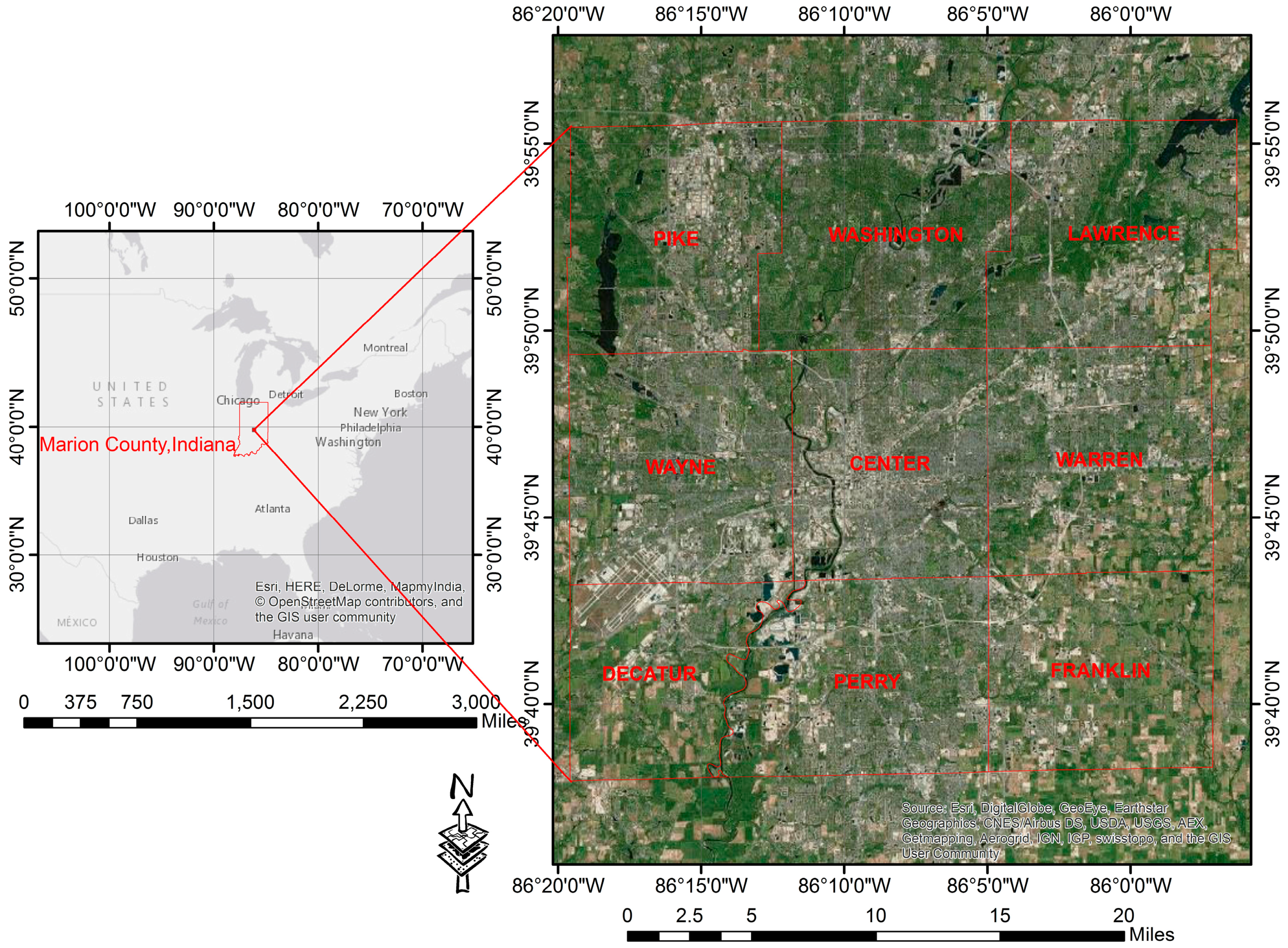
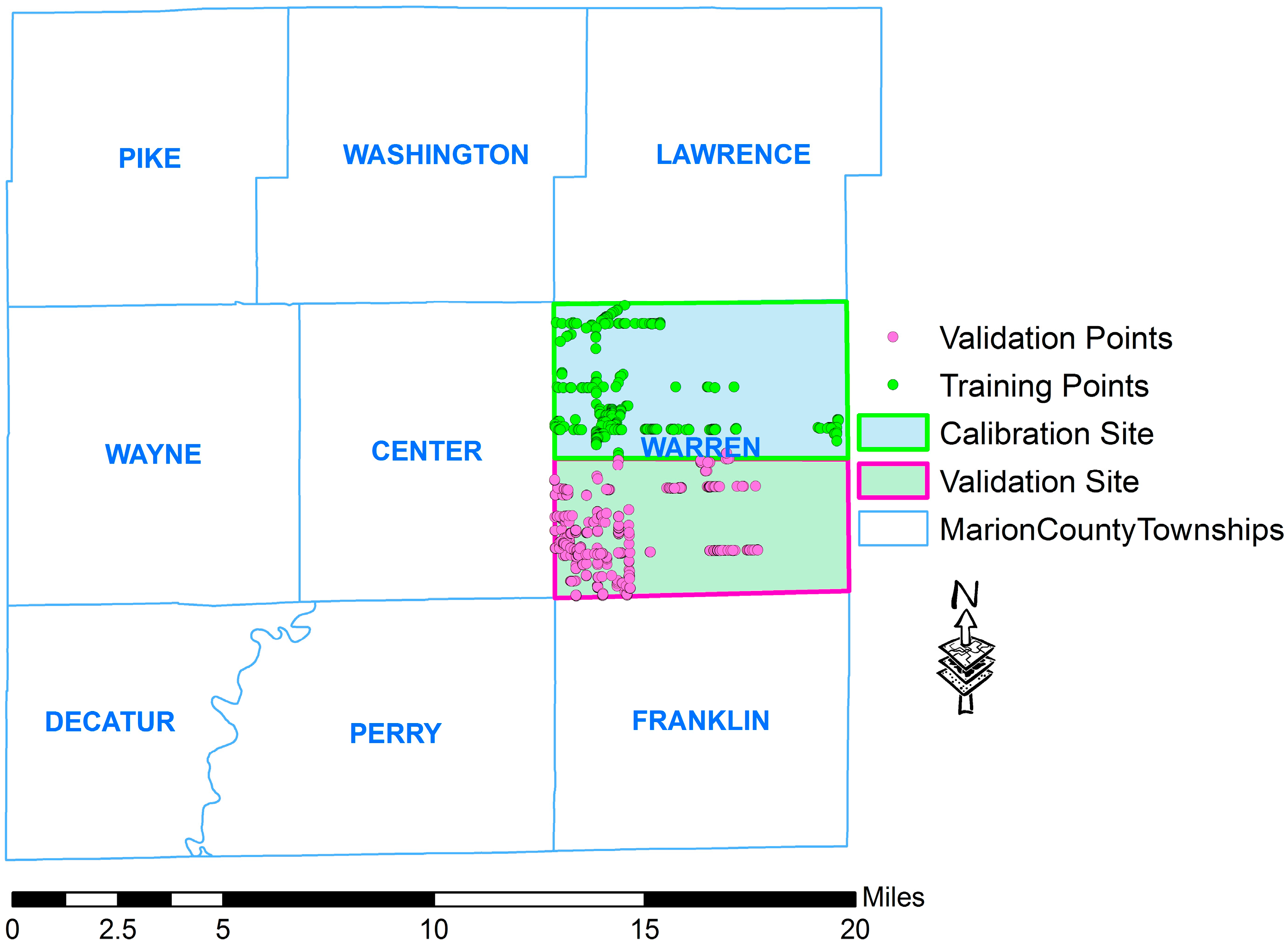
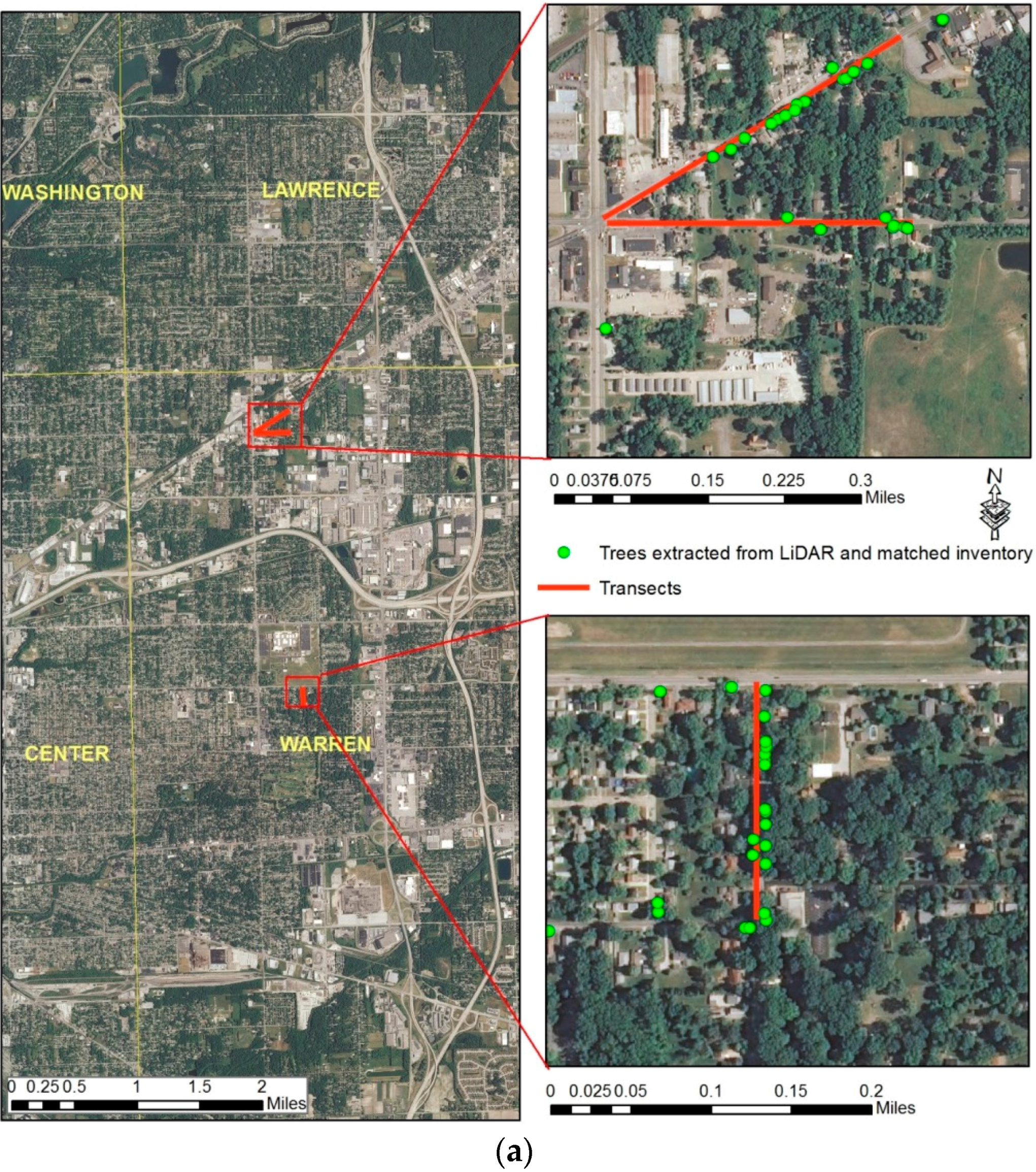
2.1. Study Area
2.2. Dataset
2.3. Methodology
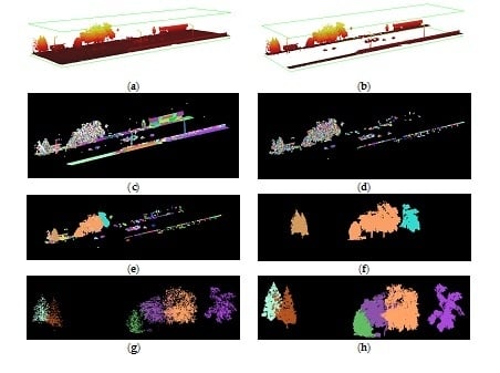
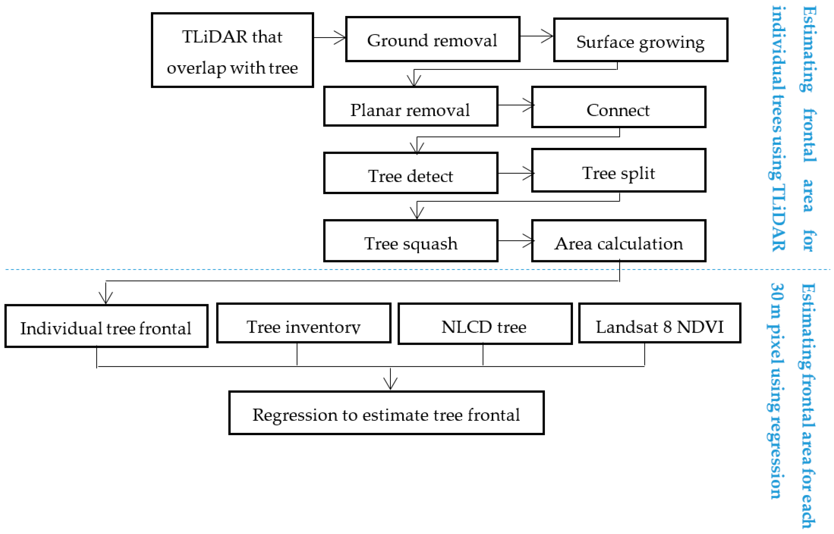
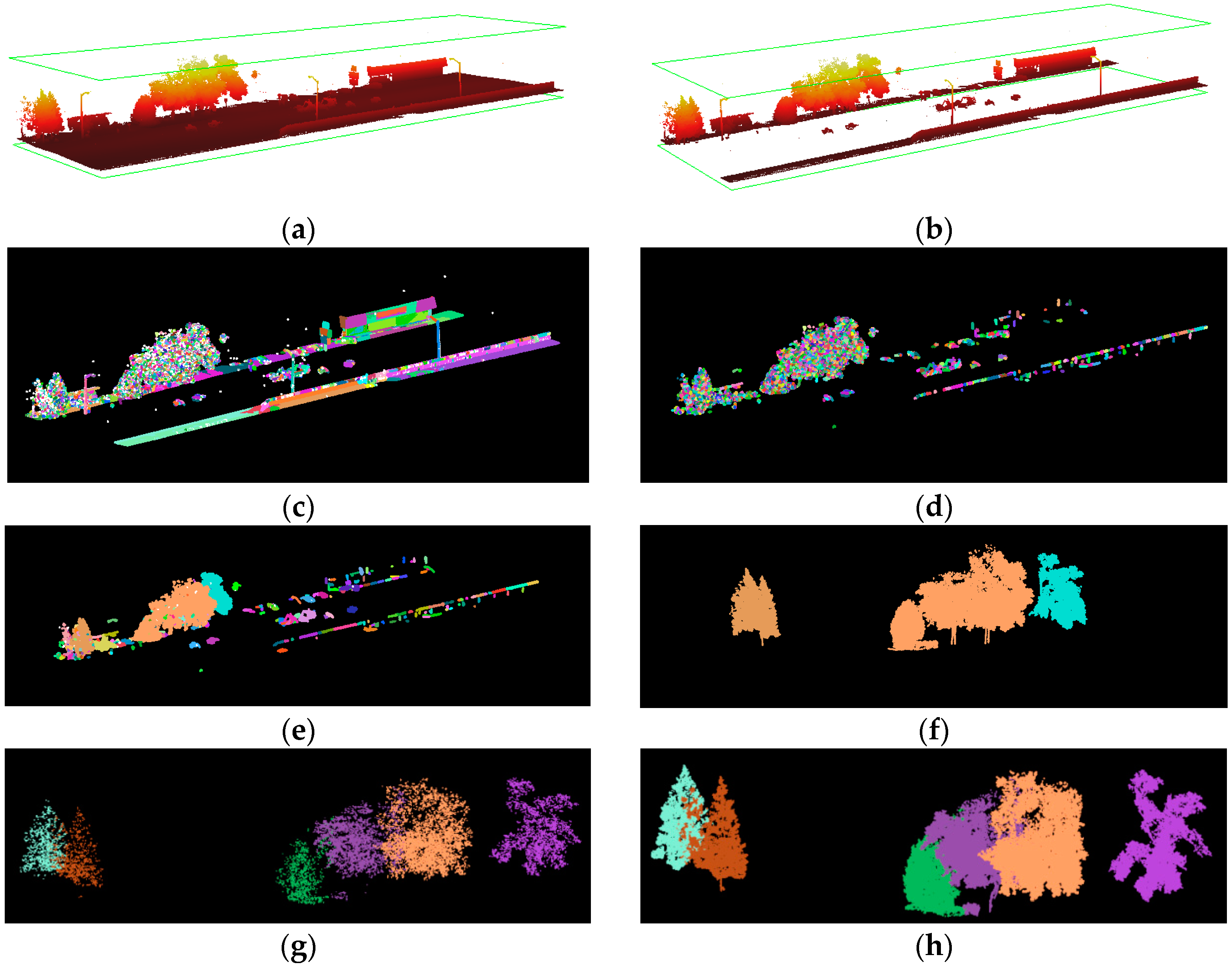
2.3.1. Estimation of Individual Tree Frontal Area
2.3.2. Green Vegetation Abundance Contributed by Trees
2.3.3. Tree Categories
2.3.4. Tree Frontal Area Estimation in 30 m Pixels
3. Results
3.1. Frontal Area Estimation for Individual Trees
3.2. Estimating Frontal Area for per 30 m Pixel
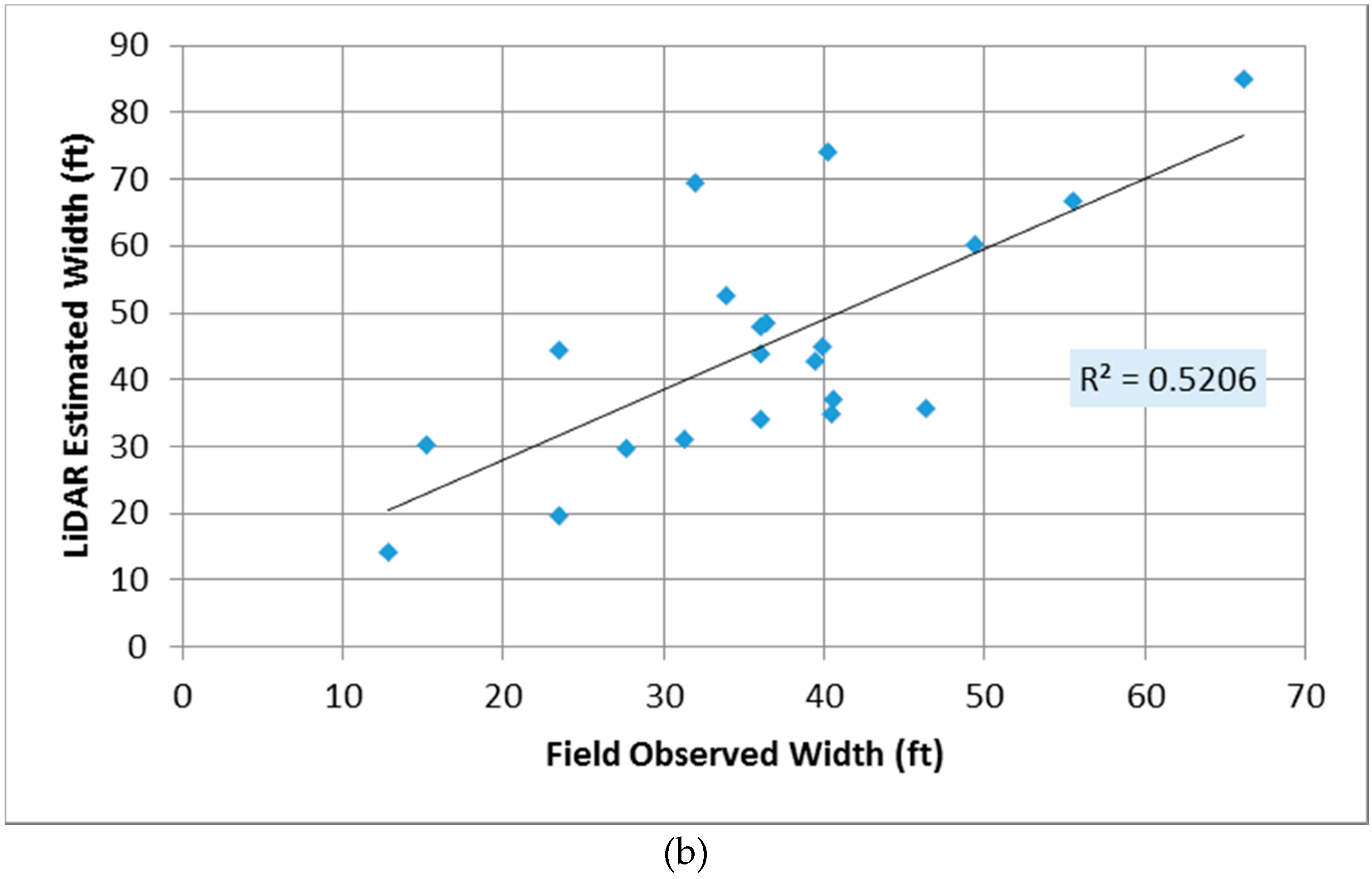
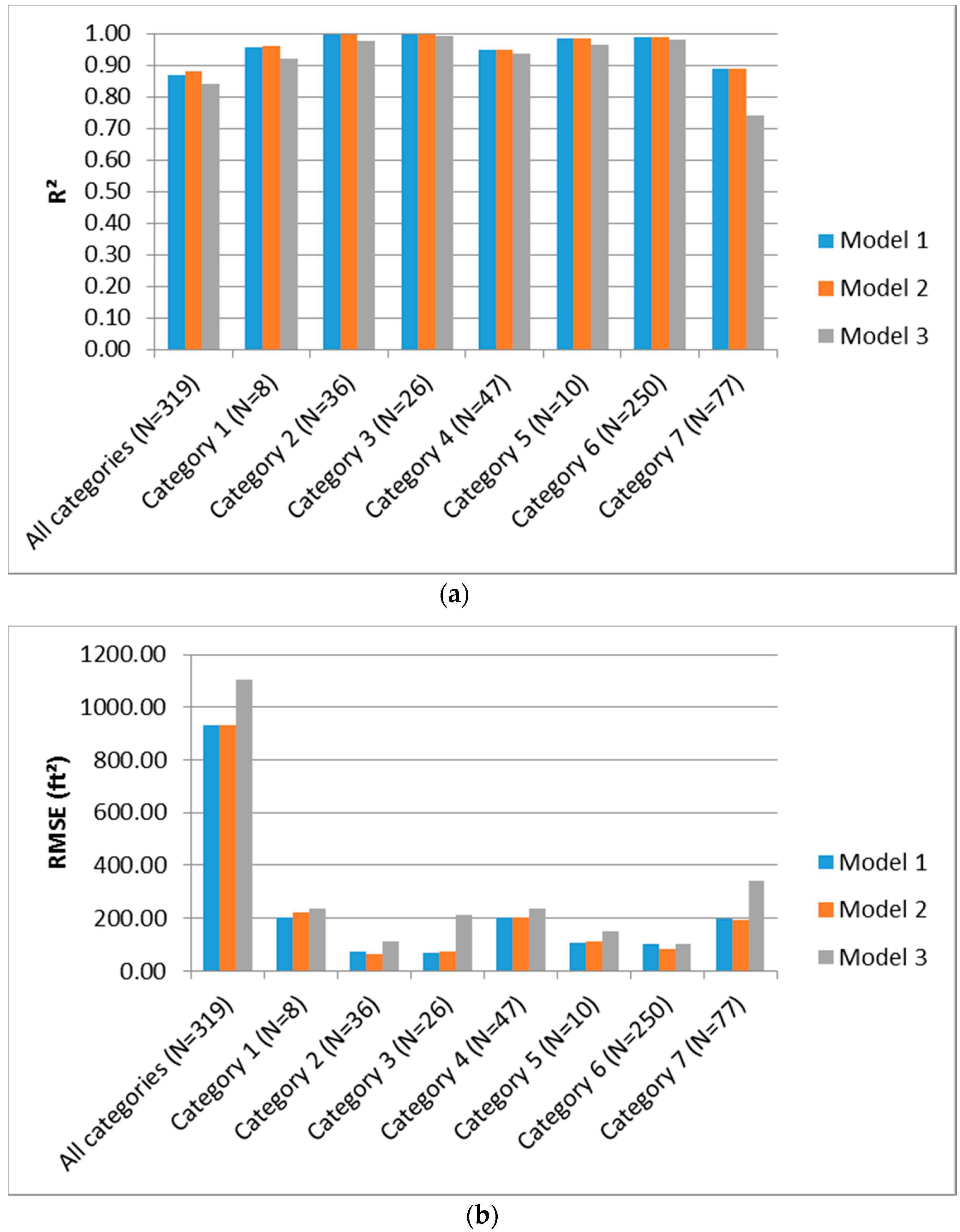
3.3. Model Validation
4. Discussion
5. Conclusions
Acknowledgments
Author Contributions
Conflicts of Interest
Appendix A

| Tree Name | Genus | Understory/Intermediate/Dominant | Broad/Sparse Canopy | Suggested Category |
|---|---|---|---|---|
| Honeysuckle, spp. | Lonicera | U | S | 1 |
| Dogwood | Cornus | U | S | 1 |
| Redbud | Cercis | U | S | 1 |
| Arborvitae spp. | Thuja | U | B | 2 |
| Autumn Olive | Elaeagnus | U | B | 2 |
| Mulberry, spp. | Morus | U | B | 2 |
| Red Mulberry | Morus | U | B | 2 |
| Russian-Olive | Elaeagnus | U | B | 2 |
| Smoketree | Cotinus | U | B | 2 |
| Staghorn Sumac | Rhus | U | B | 2 |
| White Mulberry | Morus | U | B | 2 |
| Apple | Malus | U | B | 2 |
| Lilac | Syringa | U | B | 2 |
| Serviceberry | Amelanchier | U | B | 2 |
| Sumac | Sumac | U | B | 2 |
| Zelkova | Zelkova | U | B | 2 |
| American Sycamore | Platanus | I | S | 3 |
| Ironwood | Ostrya | I | S | 3 |
| Ginkgo | Ginkgo | I | S | 3 |
| Hawthorn | Crataegus | I | S | 3 |
| Locust | Robinia | I | S | 3 |
| Pear | Pyrus | I | S | 3 |
| Plane tree | Platanus | I | S | 3 |
| Poplar | Poplar | I | S | 3 |
| Black Cherry | Prunus | I | B | 4 |
| Cherry, Japanese flowering | Prunus | I | B | 4 |
| Cherry, Plum, Peach | Prunus | I | B | 4 |
| Cherry, sweet | Prunus | I | B | 4 |
| Chokecherry | Prunus | I | B | 4 |
| Golden Raintree | Koelreuteria | I | B | 4 |
| Higan Cherry | Prunus | I | B | 4 |
| Mimosa | Albizia | I | B | 4 |
| Northern Catalpa | Catalpa | I | B | 4 |
| Osage-Orange | Maclura | I | B | 4 |
| Persimmon | Diospyros | I | B | 4 |
| plum, cherry | Prunus | I | B | 4 |
| Yellowwood | Prunus | I | B | 4 |
| Buckeye | Aesculus | I | B | 4 |
| Magnolia | Magnolia | I | B | 4 |
| Prunus | Prunus | I | B | 4 |
| Sweetgum | Liquidambar | I | B | 4 |
| Willow | Salix | I | B | 4 |
| Ash, pumpkin | Fraxinus | D | B | 5 |
| Kentucky Coffeetree | Gymnocladus | D | S | 5 |
| Birch | Betula | D | S | 5 |
| American Linden | Tilia | D | B | 6 |
| Baldcypress ‘Shawnee Brave’ | Taxodium | D | S | 6 |
| Boxelder | Acer | D | B | 6 |
| Chancelleor Linden | Tilia | D | B | 6 |
| Eastern Cottonwood | Populus | D | S | 6 |
| Hackberry | Celtis | I | B | 6 |
| Horsechestnut | Aesculus | D | B | 6 |
| Pecan | Carya | D | B | 6 |
| Silver Linden | Tilia | D | B | 6 |
| Tree-Of-Heaven | Ailanthus | I | B | 6 |
| Ash | Fraxinus | D | B | 6 |
| Beech | Fagus | D | B | 6 |
| Elm | Ulmus | D | B | 6 |
| Hickory | Carya | D | B | 6 |
| Maple | Acer | D | B | 6 |
| Oak | Quercus | D | B | 6 |
| Tupelo | Nyssa | D | B | 6 |
| Walnut | Juglans | D | B | 6 |
| Dawn Redwood | Metasequoia | D | B | 7 |
| Douglas Fir | Pseudotsuga | D | B | 7 |
| White Fir | Abies | D | B | 7 |
| Conifer | D | B | 7 |
References
- Weng, Q. Thermal infrared remote sensing for urban climate and environmental studies: Methods, applications, and trends. ISPRS J. Phtogramm. 2009, 64, 335–344. [Google Scholar] [CrossRef]
- Vancutsem, C.; Ceccato, P.; Dinku, T.; Connor, S.J. Evaluation of MODIS land surface temperature data to estimate air temperature in different ecosystems over Africa. Remote. Sens. Environ. 2010, 114, 449–465. [Google Scholar] [CrossRef]
- Ho, H.C.; Knudby, A.; Sirovyak, P.; Xu, Y.; Hodul, M.; Henderson, S.B. Mapping maximum urban air temperature on hot summer days. Remote. Sens. Environ. 2014, 154, 38–45. [Google Scholar] [CrossRef]
- Norman, J.M.; Kustas, W.P.; Humes, K.S. A two source approach for estimating soil and vegetation energy fluxes in observations of directional radiometric surface temperature. Agric. For. Meteorol. 1995, 77, 263–293. [Google Scholar] [CrossRef]
- Kato, S.; Yamaguchi, Y. Estimation of storage heat flux in an urban area using ASTER data. Remote. Sens. Environ. 2007, 110, 1–17. [Google Scholar] [CrossRef]
- Weng, Q.; Hu, X.; Quattrochi, D.A.; Liu, H. Assessing intra-urban surface energy fluxes using remotely sensed ASTER imagery and routine meteorological data: A case study in Indianapolis, U.S.A. IEEE J. Sel. Top. Appl. Earth Obs. Remote. Sens. 2013, 7, 4046–4057. [Google Scholar] [CrossRef]
- Grimmond, C.S.B.; Cleugh, H.A.; Oke, T.R. An objective urban heat storage model and its comparison with other schemes. Atmos. Environ. 1991, 25B, 311–326. [Google Scholar] [CrossRef]
- Stull, R.B. An Introduction to Boundary Layer Meteorology; Kluwer Academic Publisher: Dordrecht, The Netherlands, 1988. [Google Scholar]
- Grimmond, C.S.B.; Oke, T.R. Aerodynamic properties of urban areas derived from analysis of surfaces form. J. Appl. Meteorol. 1999, 38, 1262–1292. [Google Scholar] [CrossRef]
- Paul-Limoges, E.; Christen, A.; Coops, N.C.; Black, T.A.; Trofymow, J.A. Estimation of aerodynamic roughness of a harvested Douglas-fir forest using airborne LiDAR. Remote. Sens. Environ. 2013, 136, 225–233. [Google Scholar] [CrossRef]
- Bottema, M. Urban roughness modelling in relation to pollutant dispersion. Atmos. Environ. 1997, 31, 3059–3075. [Google Scholar] [CrossRef]
- Raupach, M.R. Simplified expressions for vegetation roughness length and zero-plane displacement as functions of canopy height and area index. Bound.-Layer Meteorol. 1994, 71, 211–216. [Google Scholar] [CrossRef]
- Macdonald, R.W.; Griffiths, R.F.; Hall, D.J. An improved method for estimation of surface roughness of obstacle arrays. Atmos. Environ. 1998, 32, 1857–1864. [Google Scholar] [CrossRef]
- Burian, S.J.; Brown, M.J.; Linger, S.P. Morphological Analyses Using 3D Building Database: Los Angeles, California; Los Alamos National Laboratory: Los Angeles, CA, USA, 2002.
- Burian, S.J.; Han, W.S.; Brown, M.J. Morphological Analyses Using 3D Building Databases: Houston, Texas; Los Alamos National Laboratory: Los Angeles, CA, USA, 2003.
- Burian, S.J.; Han, W.S.; Brown, M.J. Morphological Analyses Using 3D Building Databases: Oklahoma City, Oklahoma; Los Alamos National Laboratory: Los Angeles, CA, USA, 2003.
- Antonarakis, A.S.; Richards, K.S.; Brasington, J.; Bithell, M. Leafless roughness of complex tree morphology using terrestrial LiDAR. Water Resour. Res. 2009, 45. [Google Scholar] [CrossRef]
- Vosselman, G.; Gorte, B.; Sithole, G.; Rabbani, T. Recognizing structure in laser scanner point clouds. Int. Arch. Photogramm. Remote. Sens. Spat. Inf. Sci. 2004, 46, 33–38. [Google Scholar]
- Lafarge, F.; Descombes, X.; Zerubia, J.; Pierrot-Deseilligny, M. Automatic building extraction from DEMs using an object approach and application to the 3D-city modeling. ISPRS J. Photogramm. 2008, 63, 365–381. [Google Scholar] [CrossRef] [Green Version]
- Zhou, Q. 3D Urban Modeling from City-Scale Aerial LiDAR Data; Doctoral Dissertation, University of South California: Los Angeles, CA, USA, 2012. [Google Scholar]
- Sun, S. Automatic 3D Building Detection and Modeling from Airborne LiDAR Point Clouds; Rochester Institute of Technology: Rochester, NY, USA, 2013. [Google Scholar]
- Sun, S.; Salvaggio, C. Aerial 3D building detection and modeling from Airborne LiDAR point clouds. IEEE J. Sel. Top. Appl. 2013, 6, 1440–1449. [Google Scholar] [CrossRef]
- Rutzinger, M.; Pratihast, A.K.; Oude Elberink, S.; Vosselman, G. Detection and modeling of 3D trees from mobile laser scanning data. Int. Arch. Photogramm. Remote. Sens. Spat. Inf. Sci. 2010, XXXVIII, 520–525. [Google Scholar]
- Chen, Q.; Baldocchi, D.; Gong, P.; Kelly, M. Isolating individual trees in a Savanna woodland using small footprint LiDAR data. Photogramm. Eng. Remote. Sens. 2006, 72, 923–932. [Google Scholar] [CrossRef]
- Alonzo, M.; Bookhagen, B.; Roberts, D.A. Urban tree species mapping using hyperspectral and LiDAR data fusion. Remote. Sens. Environ. 2014, 148, 70–83. [Google Scholar] [CrossRef]
- Li, W.; Guo, Q.; Jakubowski, M.K.; Kelly, M. A new method for segmenting individual trees from the LiDAR point cloud. Photogramm. Eng. Remote. Sens. 2012, 78, 75–84. [Google Scholar] [CrossRef]
- Lu, X.; Guo, Q.; Li, W.; Flanagan, J. A bottom-up approach to segment individual deciduous trees using leaf-off LiDAR point cloud data. ISPRS J. Phtogramm. 2014, 94, 1–12. [Google Scholar] [CrossRef]
- Jennings, S.B.; Brown, N.D.; Sheil, D. Assessing forest canopies and understorey illumination: Canopy closure, canopy cover and other measures. Forestry 1999, 71, 59–73. [Google Scholar] [CrossRef]
- Fahey, R.T.; Bialecki, M.B.; Carter, D.R. Tree growth and resilience to extreme drought across an urban land-use gradient. Arboric. Urban For. 2013, 39, 279–285. [Google Scholar]
- Wu, B.; Yu, B.; Yue, W.; Shu, S.; Tan, W.; Hu, C.; Huang, Y.; Wu, J.; Liu, H.A. Voxel-based method for automated identification and morphological parameters estimation of individual street trees from mobile laser scanning data. Remote. Sens. 2013, 5, 584–611. [Google Scholar] [CrossRef]
- Burnham, K.P.; Anderson, D.R. Model Selection and Multimodel Inference: A practical Information-Theoretic Approach, 2nd ed.; Springer-Verlag: New York, NY, USA, 2002. [Google Scholar]


| Suggested Category | Understory/Intermediate /Dominant | Broad/Sparse Canopy | Examples of Trees |
|---|---|---|---|
| 1 | U | S | Honeysuckle, Dogwood, Redbud |
| 2 | U | B | Arborvitae, Autumn Olive, Mulberry |
| 3 | I | S | American Sycamore, Poplar, Ginkgo |
| 4 | I | B | Black Cherry, Buckeye, Willow |
| 5 | D | B | Birch, Kentucky Coffeetree |
| 6 | D | S | Ash, Beech, Elm, Maple, Walnut |
| 7 | D | B | Dawn Redwood, Conifer, Douglas Fir |
| Independent Variables | Pearson Correlation | Data Source |
|---|---|---|
| Sum DBH | 0.519 | Tree Inventory |
| # of trees with two abnormal diagnoses | 0.624 | Tree Inventory |
| # of trees in poor condition | 0.609 | Tree Inventory |
| # of trees performed large tree clean | 0.518 | Tree Inventory |
| # of trees with utility maintenance | 0.608 | Tree Inventory |
| # of tree with sidewalk heaved <3/4 inch | 0.661 | Tree Inventory |
| # of trees in Single-family residential land | 0.568 | Tree Inventory |
| # of trees with <4 in defect | 0.569 | Tree Inventory |
| Sum Crown Base Area | 0.991 | Terrestrial LiDAR |
| Sum Height | 0.853 | Terrestrial LiDAR |
| Sum width (EW length) | 0.922 | Terrestrial LiDAR |
| Sum width (NS length) | 0.901 | Terrestrial LiDAR |
© 2016 by the authors; licensee MDPI, Basel, Switzerland. This article is an open access article distributed under the terms and conditions of the Creative Commons Attribution (CC-BY) license (http://creativecommons.org/licenses/by/4.0/).
Share and Cite
Jiang, Y.; Weng, Q.; Speer, J.H.; Baker, S. Estimating Tree Frontal Area in Urban Areas Using Terrestrial LiDAR Data. Remote Sens. 2016, 8, 401. https://0-doi-org.brum.beds.ac.uk/10.3390/rs8050401
Jiang Y, Weng Q, Speer JH, Baker S. Estimating Tree Frontal Area in Urban Areas Using Terrestrial LiDAR Data. Remote Sensing. 2016; 8(5):401. https://0-doi-org.brum.beds.ac.uk/10.3390/rs8050401
Chicago/Turabian StyleJiang, Yitong, Qihao Weng, James H. Speer, and Steven Baker. 2016. "Estimating Tree Frontal Area in Urban Areas Using Terrestrial LiDAR Data" Remote Sensing 8, no. 5: 401. https://0-doi-org.brum.beds.ac.uk/10.3390/rs8050401