
Application of Open Source Coding Technologies in the Production of Land Surface Temperature (LST) Maps from Landsat: A PyQGIS Plugin


Abstract
:
1. Introduction
2. Materials and Methods
2.1. Data
2.1.1. Landsat
2.1.2. Meteorological Data
2.1.3. Plugin Development Tools
2.2. Methodology
2.2.1. Conversion of Digital Numbers to at-Sensor Radiance
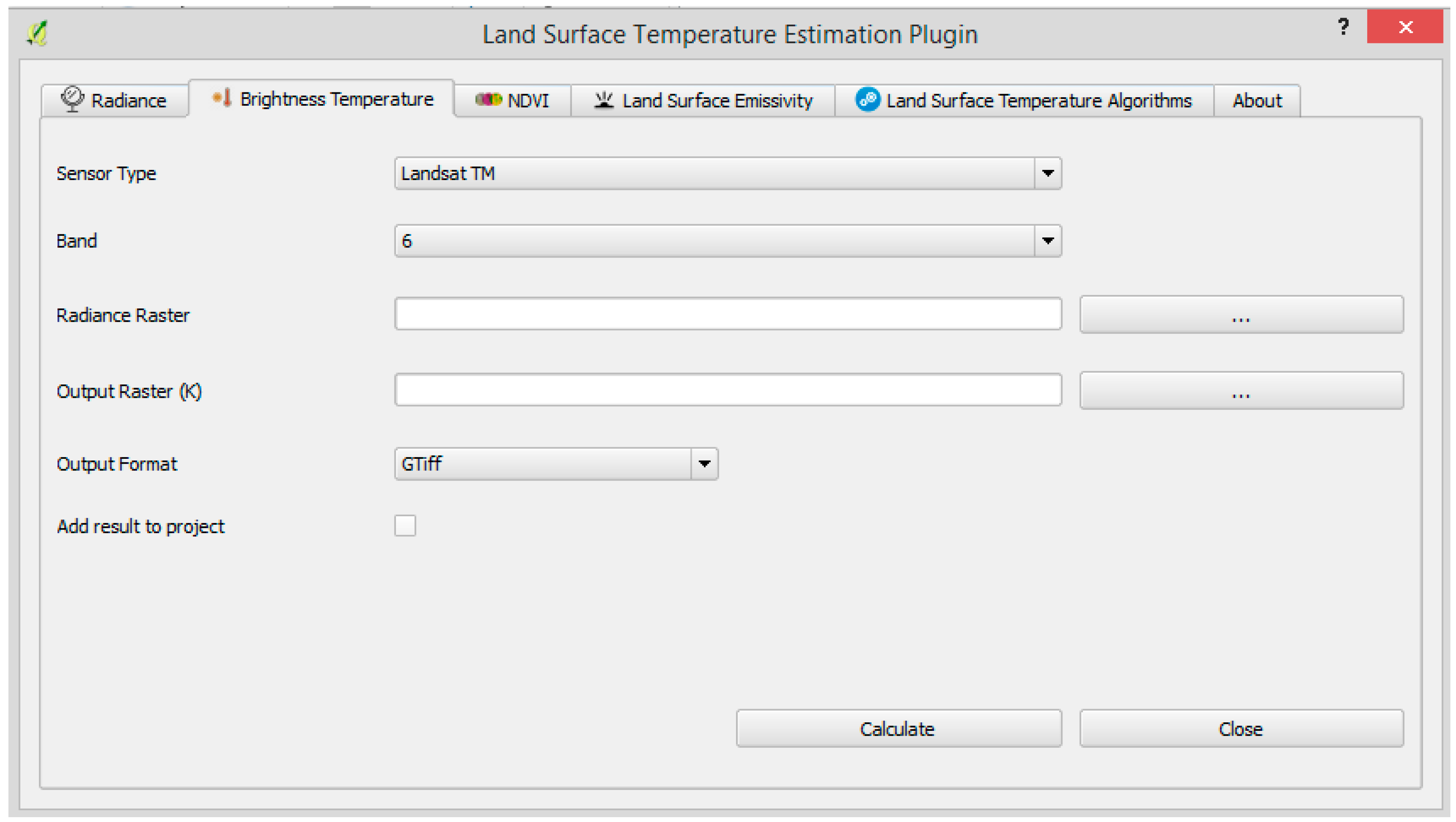
2.2.2. Computation of Brightness Temperature
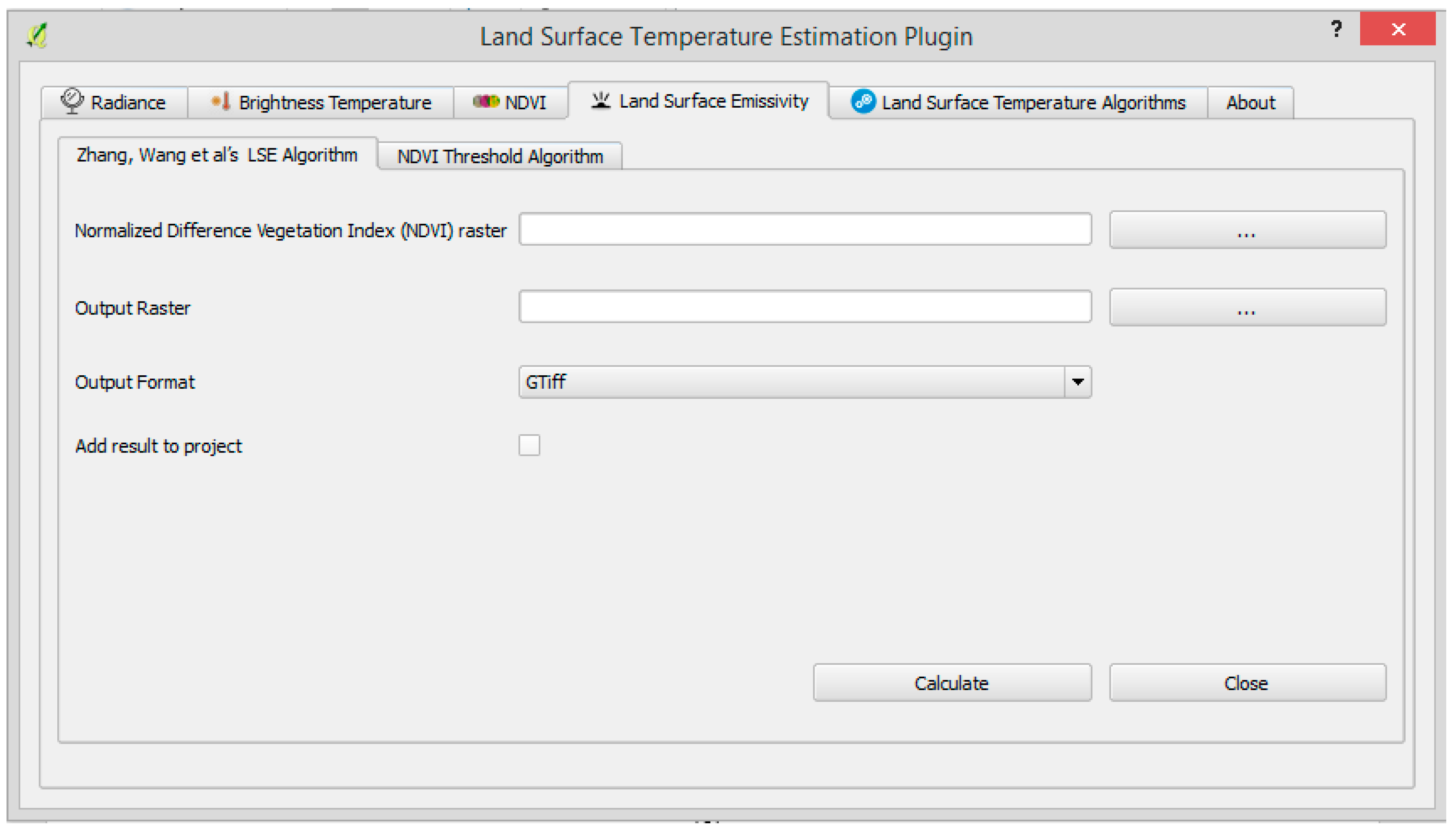
2.2.3. Determination of Land Surface Emissivity (LSE)
- Algorithm based on the NDVI image
- NDVI threshold LSE estimation algorithm
- (NDVI < NDVIs) in this scenario, a pixel is considered to be composed of bare soil or rock, therefore, the LSE of soil is assigned to the pixel.
- (NDVI > NDVIs) in this scenario, a pixel is considered to be composed of full vegetation cover, therefore, the LSE of vegetation is assigned to the pixel.
- (NDVIs ≤ NDVI ≤ NDVIv) in this scenario, a pixel is considered to be composed of a mixture of vegetation and rocks/soil; therefore, the authors in [22] introduced Equation (6) to represent the relationship between NDVI and LSE.
2.2.4. Estimation of Atmospheric Transmittance, Upwelling and Down-Welling Radiance
2.2.5. Determination of Near Surface Air Temperature
2.2.6. Determination of Atmospheric Water Vapor
2.2.7. Brightness Temperature Emissivity/Atmospheric Correction
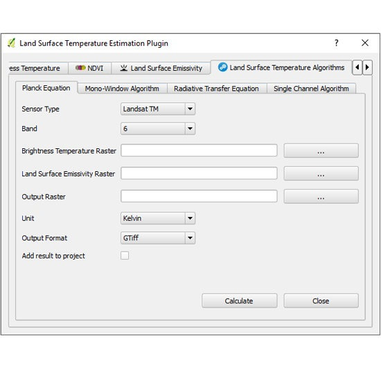
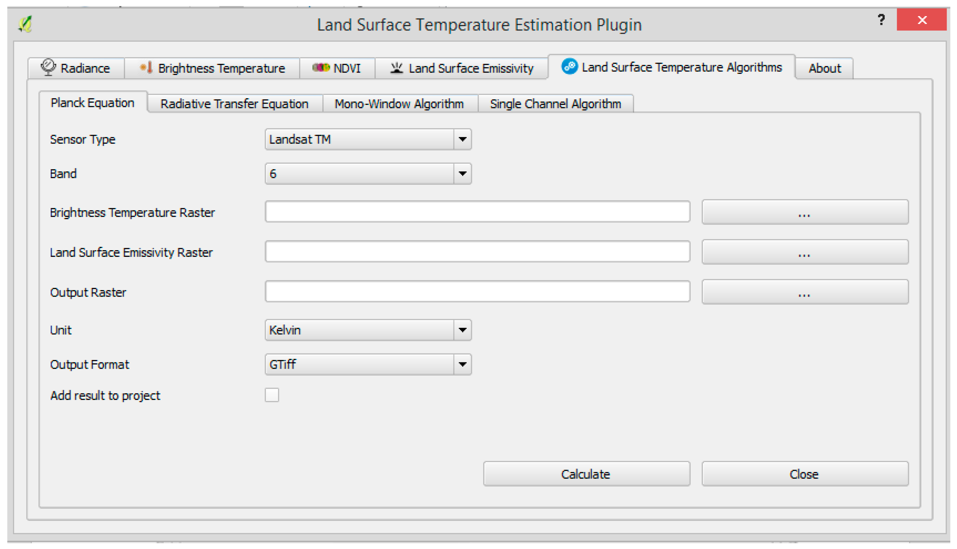
Inversion of Planck’s Function
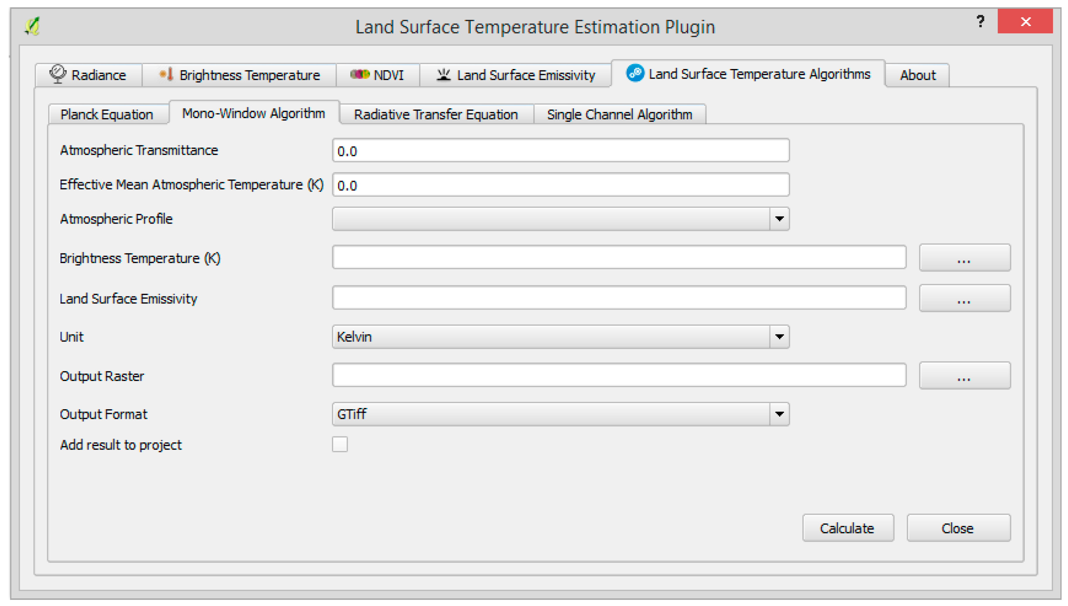
Mono-Window Algorithm (MWA)
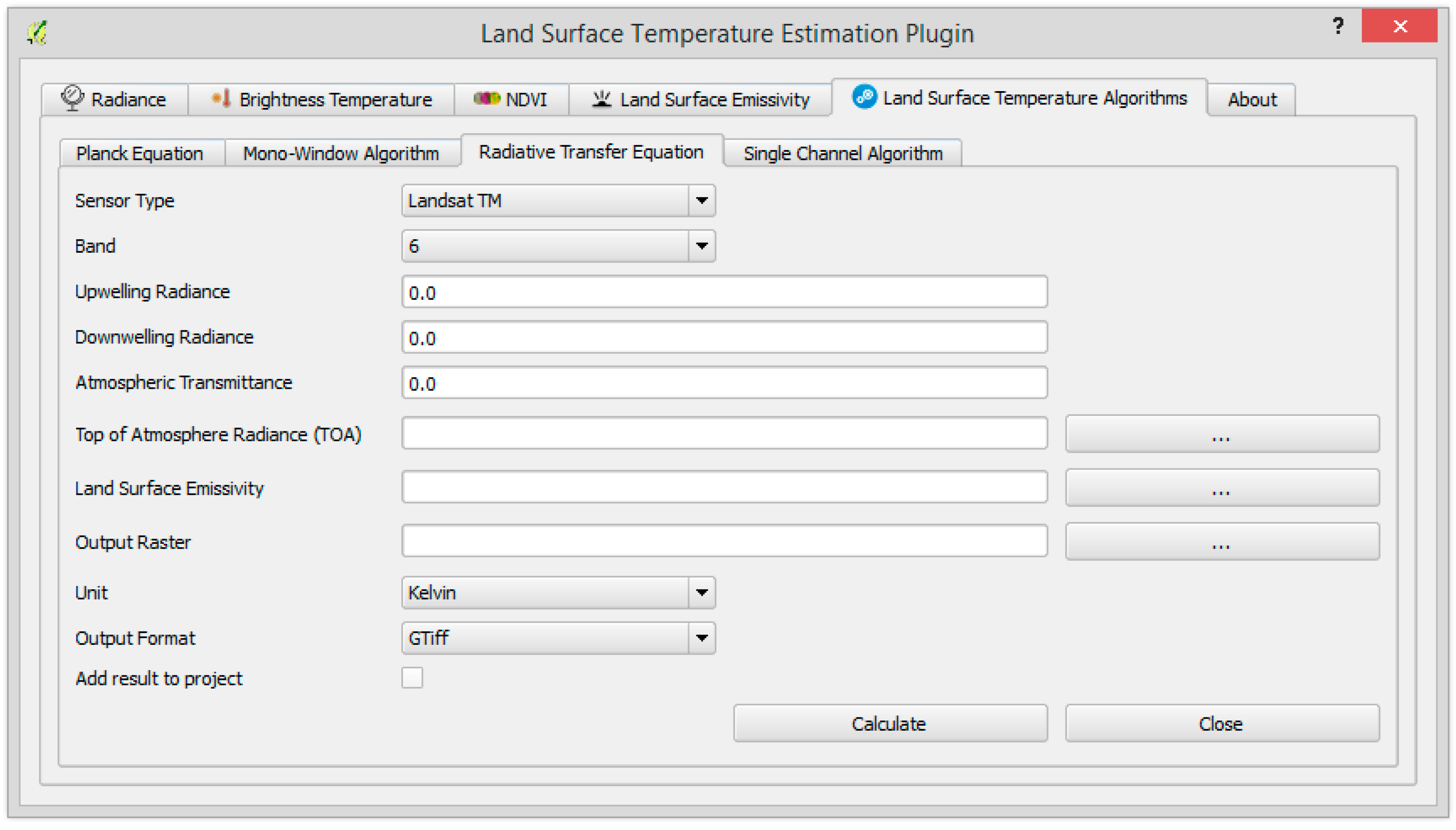
Radiative Transfer Equation (RTE)
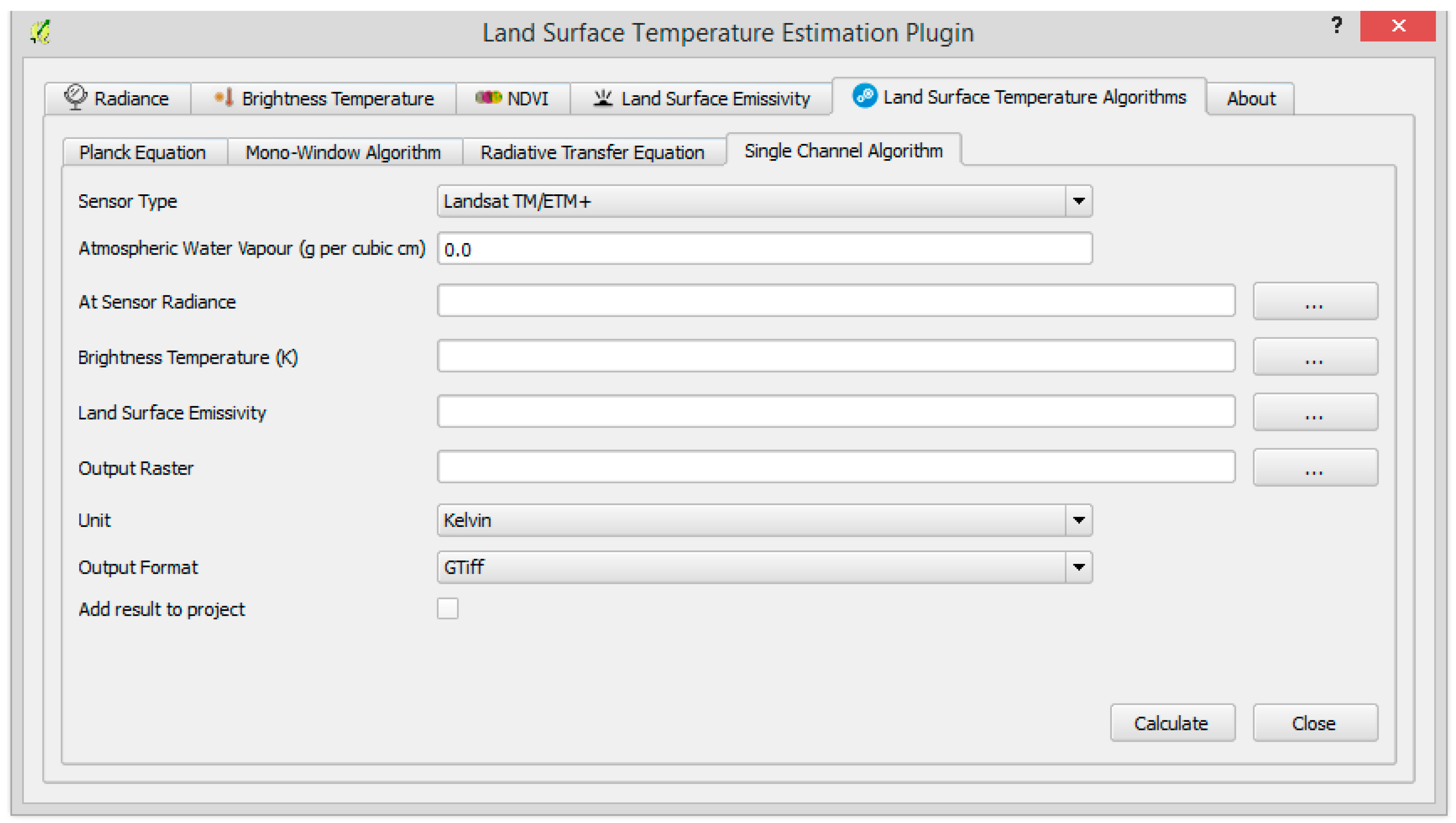
Single Channel Algorithm (SCA)
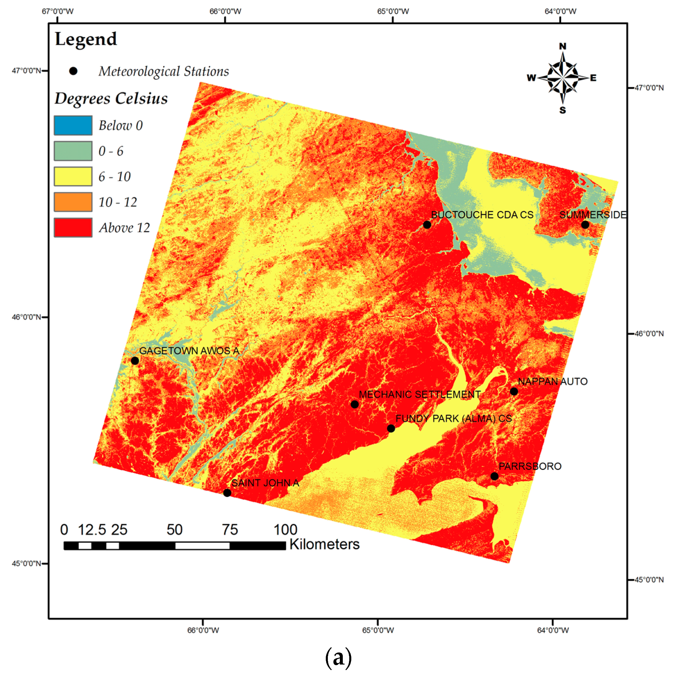
3. Results
4. Discussion
5. Conclusions
Acknowledgments
Author Contributions
Conflicts of Interest
Abbreviations
| NST | Near Surface Temperature |
| RH | Relative Humidity |
| VNIR | Visible and Near Infrared |
| TIR | Thermal Infrared |
| LST | Land Surface Temperature |
| LSE | Land Surface Emissivity |
| SCA | Single Channel Algorithm |
| MWA | Mono Window Algorithm |
| RTE | Radiative Transfer Equation |
| RS | Remote Sensing |
| GIS | Geographic Information Systems |
| NDVI | Normalized Difference Vegetation Index |
| TOA | Top of Atmosphere |
| EOS | Earth Observation Satellites |
| USGS | United States Geological Survey |
| UTC | Coordinated Universal Time |
| GDAL | Geospatial Data Abstraction Library |
| DN | Digital Numbers |
| K | Kelvin |
| OLI | Operational Land Imager |
| TM | Thematic Mapper |
| ETM+ | Enhanced Thematic Mapper Plus |
| NASA | National Aeronautics and Space Administration |
| NCEP | National Centers for Environmental Prediction |
References
- Wu, P.; Shen, H.; Zhang, L.; Göttsche, F.-M. Integrated fusion of multi-scale polar-orbiting and geostationary satellite observations for the mapping of high spatial and temporal resolution land surface temperature. Remote Sens. Environ. 2015, 156, 169–181. [Google Scholar]
- Li, Z.-L.; Tang, B.-H.; Wu, H.; Ren, H.; Yan, G.; Wan, Z.; Trigo, I.F.; Sobrino, J.A. Satellite-derived land surface temperature: Current status and perspectives. Remote Sens. Environ. 2013, 131, 14–37. [Google Scholar] [CrossRef]
- Pandya, M.R.; Shah, D.B.; Trivedi, H.J.; Darji, N.P.; Ramakrishnan, R.; Panigrahy, S.; Parihar, J.S.; Kirankumar, A.S. Retrieval of land surface temperature from the Kalpana-1 VHRR data using a single-channel algorithm and its validation over western India. ISPRS J. Photogramm. Remote Sens. 2014, 94, 160–168. [Google Scholar] [CrossRef]
- Jiménez-Muñoz, J.-C.; Sobrino, J.A. Split-window coefficients for land surface temperature retrieval from low-resolution thermal infrared sensors. IEEE Geosci. Remote Sens. Lett. 2008, 5, 806–809. [Google Scholar] [CrossRef]
- Jiménez-Muñoz, J.C.; Sobrino, J.A. A single-channel algorithm for land-surface temperature retrieval from aster data. IEEE Geosci. Remote Sens. Lett. 2010, 7, 176–179. [Google Scholar] [CrossRef]
- Qin, Z.-H.; Karnieli, A.; Berliner, P. A mono-window algorithm for retrieving land surface temperature from landsat TM data and its application to the Israel-Egypt border region. Int. J. Remote Sens. 2001, 22, 3719–3746. [Google Scholar] [CrossRef]
- Team, Q.D. QGIS Python Plugins Repository. Available online: http://plugins.qgis.org/ (accessed on 11 May 2016).
- USGS. Earth Explorer. Available online: http://earthexplorer.usgs.gov/ (accessed on 5 May 2016).
- Historical Data. Available online: http://climate.weather.gc.ca/ (accessed on 5 May 2016).
- USGS. Using the USGS Landsat 8 Product. Available online: http://landsat.usgs.gov/Landsat8_Using_Product.php (accessed on 9 November 2014).
- USGS. Landsat 8 (L8) Operational Land Imager (OLI) and Thermal Infrared Sensor (TIRS). Available online: http://landsat.usgs.gov/calibration_notices.php (accessed on 9 February 2016).
- Barsi, J.A.; Schott, J.R.; Hook, S.J.; Raqueno, N.G.; Markham, B.L.; Radocinski, R.G. Landsat-8 thermal infrared sensor (TIRS) vicarious radiometric calibration. Remote Sens. 2014, 6, 11607–11626. [Google Scholar] [CrossRef]
- USGS. Frequently Asked Questions about the Landsat Missions. Available online: http://landsat.usgs.gov/how_is_radiance_calculated.php (accessed on 24 March 2016).
- Finn, M.P.; Reed, M.D.; Yamamoto, K.H. A Straight forward Guide for Processing Radiance and Reflectance for eo-1 ALI, Landsat 5 tm, Landsat 7 ETM+, and Aster; Unpublished Report; USGS/Center of Excellence for Geospatial Information Science: Washington, DC, USA, 2012. [Google Scholar]
- Kruse, P.W.; McGlauchlin, L.D.; McQuistan, R.B. Elements of Infrared Technology: Generation, Transmission and Detection; Wiley: New York, NY, USA, 1962; Volume 1962. [Google Scholar]
- Wang, S.L.L. Chapter 8—Land-surface temperature and thermal infrared emissivity. In Advanced Remote Sensing; Wang, S.L.L., Ed.; Academic Press: Boston, FL, USA, 2012; pp. 235–271. [Google Scholar]
- Tang, B.-H.; Wu, H.; Li, C.; Li, Z.-L. Estimation of broadband surface emissivity from narrowband emissivities. Opt. Express 2011, 19, 185–192. [Google Scholar] [CrossRef] [PubMed]
- Wang, F.; Qin, Z.; Song, C.; Tu, L.; Karnieli, A.; Zhao, S. An improved mono-window algorithm for land surface temperature retrieval from landsat 8 thermal infrared sensor data. Remote Sens. 2015, 7, 4268–4289. [Google Scholar] [CrossRef]
- Vandegriend, A.; Owe, M.; Vugts, H.; Ramothwa, G. Botswana Water and Surface Energy Balance Research Program. Part 1: Integrated Approach and Field Campaign Results; NASA Goddard Space Flight Center: Greenbelt, MD, USA, 1992. [Google Scholar]
- Srivastava, P.K.; Han, D.; Rico-Ramirez, M.A.; Bray, M.; Islam, T.; Gupta, M.; Dai, Q. Estimation of land surface temperature from atmospherically corrected landsat TM image using 6S and NCEP global reanalysis product. Environ. Earth Sci. 2014, 72, 5183–5196. [Google Scholar] [CrossRef]
- Zhang, J.; Wang, Y.; Li, Y. A C++ program for retrieving land surface temperature from the data of landsat TM/ETM+ band6. Comput. Geosci. 2006, 32, 1796–1805. [Google Scholar] [CrossRef]
- Sobrino, J.; Raissouni, N. Toward remote sensing methods for land cover dynamic monitoring: Application to morocco. Int. J. Remote Sens. 2000, 21, 353–366. [Google Scholar] [CrossRef]
- Sobrino, J.; Caselles, V.; Becker, F. Significance of the remotely sensed thermal infrared measurements obtained over a citrus orchard. ISPRS J. Photogramm. Remote Sens. 1990, 44, 343–354. [Google Scholar] [CrossRef]
- Yu, X.; Guo, X.; Wu, Z. Land surface temperature retrieval from landsat 8 TIRS—Comparison between radiative transfer equation-based method, split window algorithm and single channel method. Remote Sens. 2014, 6, 9829–9852. [Google Scholar] [CrossRef]
- Carlson, T.N.; Ripley, D.A. On the relation between NDVI, fractional vegetation cover, and leaf area index. Remote Sens. Environ. 1997, 62, 241–252. [Google Scholar] [CrossRef]
- Barsi, J.; Barker, J.L.; Schott, J.R. An atmospheric correction parameter calculator for a single thermal band earth-sensing instrument. In Proceedings of the 2003 IEEE International Geoscience and Remote Sensing Symposium, Toulouse, France, 21–25 July 2003.
- Yang, J.; Qiu, J. The empirical expressions of the relation between precipitable water and ground water vapor pressure for some areas in china. Sci. Atmos. Sin. 1996, 20, 620–626. [Google Scholar]
- Li, J. Estimating land surface temperature from landsat-5 TM. Remote Sens. Technol. Appl. 2006, 21, 322–326. [Google Scholar]
- Liu, L.; Zhang, Y. Urban heat island analysis using the landsat TM data and ASTER data: A case study in Hong Kong. Remote Sens. 2011, 3, 1535–1552. [Google Scholar] [CrossRef]
- Artis, D.A.; Carnahan, W.H. Survey of emissivity variability in thermography of urban areas. Remote Sens. Environ. 1982, 12, 313–329. [Google Scholar] [CrossRef]
- Sinha, S.; Pandey, P.C.; Sharma, L.K.; Nathawat, M.S.; Kumar, P.; Kanga, S. Remote estimation of land surface temperature for different lulc features of a moist deciduous tropical forest region. In Remote Sensing Applications in Environmental Research; Springer: Berlin, Germany; Heidelberg, Germany, 2014; pp. 57–68. [Google Scholar]
- Srivastava, P.; Majumdar, T.; Bhattacharya, A.K. Surface temperature estimation in singhbhum shear zone of India using landsat-7 ETM+ thermal infrared data. Adv. Space Res. 2009, 43, 1563–1574. [Google Scholar] [CrossRef]
- Goetz, S.; Halthore, R.; Hall, F.; Markham, B. Surface temperature retrieval in a temperate grassland with multiresolution sensors. J. Geophys. Res. 1995, 100, 25397–25410. [Google Scholar] [CrossRef]
- Wukelic, G.; Gibbons, D.; Martucci, L.; Foote, H. Radiometric calibration of landsat thematic mapper thermal band. Remote Sens. Environ. 1989, 28, 339–347. [Google Scholar] [CrossRef]
- Schott, J.R.; Volchok, W.J. Thematic mapper thermal infrared calibration. Photogramm. Eng. Remote Sens. 1985, 51, 1351–1357. [Google Scholar]
- Weng, Q.; Lu, D.; Schubring, J. Estimation of land surface temperature–vegetation abundance relationship for urban heat island studies. Remote Sens. Environ. 2004, 89, 467–483. [Google Scholar] [CrossRef]
- Barsi, J.A.; Schott, J.; Palluconi, F.D.; Helder, D.; Hook, S.; Markham, B.; Chander, G.; O’Donnell, E. Landsat tm and ETM+ thermal band calibration. Can. J. Remote Sens. 2003, 29, 141–153. [Google Scholar] [CrossRef]
- Jiménez-Muñoz, J.C.; Sobrino, J.A. A generalized single-channel method for retrieving land surface temperature from remote sensing data. J. Geophys. Res. 2003, 108. [Google Scholar] [CrossRef]
- Cresswell, M.; Morse, A.; Thomson, M.; Connor, S. Estimating surface air temperatures, from meteosat land surface temperatures, using an empirical solar zenith angle model. Int. J. Remote Sens. 1999, 20, 1125–1132. [Google Scholar] [CrossRef]
- Prihodko, L.; Goward, S.N. Estimation of air temperature from remotely sensed surface observations. Remote Sens. Environ. 1997, 60, 335–346. [Google Scholar] [CrossRef]
- Stisen, S.; Sandholt, I.; Nørgaard, A.; Fensholt, R.; Eklundh, L. Estimation of diurnal air temperature using MSG SEVIRI data in West Africa. Remote Sens. Environ. 2007, 110, 262–274. [Google Scholar] [CrossRef]
- Jiménez-Muñoz, J.; Sobrino, J. Error sources on the land surface temperature retrieved from thermal infrared single channel remote sensing data. Int. J. Remote Sens. 2006, 27, 999–1014. [Google Scholar] [CrossRef]
- Kotchenova, S.Y.; Vermote, E.F. Validation of a vector version of the 6s radiative transfer code for atmospheric correction of satellite data. Part II. Homogeneous Lambertian and anisotropic surfaces. Appl. Opt. 2007, 46, 4455–4464. [Google Scholar] [CrossRef] [PubMed]
- Berk, A.; Bernstein, L.S.; Robertson, D.C. Modtran: A Moderate Resolution Model for Lowtran; DTIC Document: Belvoir, VA, USA, 1987. [Google Scholar]


| Sensor | Date | Time (UTC) | Path | Row |
|---|---|---|---|---|
| Landsat 5 TM | 13 November 2010 | 14:57 | 009 | 028 |
| Landsat 5 TM | 31 December 2010 | 14:57 | 009 | 028 |
| Landsat 7 ETM+ | 21 November 2010 | 15:00 | 009 | 028 |
| Landsat 7 ETM+ | 23 February 2016 | 15:09 | 009 | 028 |
| Landsat 8 TIRS/OLI | 29 May 2013 | 15:09 | 009 | 028 |
| Landsat 8 TIRS/OLI | 4 June 2015 | 15:06 | 009 | 028 |
| NDVI | LSE |
|---|---|
| NDVI < −0.185 | 0.995 |
| −0.185 ≤ NDVI < 0.157 | 0.985 |
| 0.157 ≤ NDVI ≤ 0.727 | 1.009 + 0.047 × ln(NDVI) |
| NDVI > 0.727 | 0.990 |
| Terrestrial Material | Soil | Built-Up Areas | Vegetation | Water |
|---|---|---|---|---|
| Emissivity | 0.966 | 0.962 | 0.973 | 0.991 |
| Sensor Type | Date | Time (UTC) | Atmospheric Transmittance | Upwelling Radiance (W/(m2·sr·µm)) | Down-Welling Radiance (W/(m2·sr·µm)) |
|---|---|---|---|---|---|
| Landsat 5 TM | 13 November 2010 | 14:57 | 0.89 | 0.72 | 1.20 |
| Landsat 5 TM | 31 December 2010 | 14:57 | 0.89 | 0.58 | 0.97 |
| Landsat 7 ETM+ | 21 November 2010 | 15:00 | 0.96 | 0.18 | 0.31 |
| Landsat 7 ETM+ | 23 February 2016 | 15:09 | 0.97 | 0.11 | 0.20 |
| Landsat 8 TIRS | 4 June 2015 | 15:06 | 0.87 | 0.91 | 1.52 |
| Landsat 8 TIRS | 29 May 2013 | 15:09 | 0.89 | 0.72 | 1.22 |
| Atmospheres | Linear Relations Equations |
|---|---|
| For USA 1976 | Ta = 25.9396 + 0.88045T0 |
| Tropical model | Ta = 17.9769 + 0.91715T0 |
| Mid-latitude Summer | Ta = 16.0110 + 0.92621T0 |
| Mid-latitude winter | Ta = 19.2704 + 0.91118T0 |
| Station Name | Latitude | Longitude | Elevation (Meters) | NST (°C) at 12:00 | RH (%) | MWA (°C) | PLANCK (°C) | RTE (°C) | SCA (°C) |
|---|---|---|---|---|---|---|---|---|---|
| Mechanic Settlement | 45°41′37.040″N | 65°09′54.040″W | 403 | −3.1 | 99 | −4.75 | −4.70 | −4.55 | −5.56 |
| Fundy Park (Alma) Cs | 45°36′00.000″N | 64°57′00.000″W | 42.7 | 3.6 | 62 | −0.91 | −1.29 | −0.73 | −2.17 |
| Buctouche Cda Cs | 46°25′49.006″N | 64°46′05.009″W | 35.9 | −0.9 | 78 | −8.06 | −7.64 | −7.85 | −8.48 |
| Nappan Auto | 45°45′34.400″N | 64°14′29.200″W | 19.8 | −7.9 | 73 | −3.46 | −3.55 | −3.26 | −4.42 |
| Saint John A | 45°19′05.000″N | 65°53′08.050″W | 108.8 | −0.2 | 69 | −0.29 | −0.73 | −0.11 | −1.62 |
| Parrsboro | 45°24′48.000″N | 64°20′49.000″W | 30.9 | 2.1 | 68 | −0.29 | −0.73 | −0.11 | −1.62 |
| Gagetown A | 45°50′00.000″N | 66°26′00.000″W | 50.6 | −2.2 | 79 | −0.91 | −1.29 | −0.73 | −2.17 |
| Gagetown Awos A | 45°50′20.000″N | 66°26′59.000″W | 50.6 | −1 | 77 | −0.29 | −0.73 | −0.11 | −1.62 |
| Summerside | 46°26′28.000″N | 63°50′17.000″W | 12.2 | −0.9 | 78 | −3.46 | −3.55 | −3.26 | −4.42 |
| Mechanic Settlement | 45°41′37.040″N | 65°09′54.040″W | 403 | −3.1 | 99 | −4.75 | −4.70 | −4.55 | −5.56 |
| Root Mean Square Error (RMSE) | 2.67 | 2.78 | 2.64 | 3.17 |
| Station Name | Latitude | Longitude | Elevation (Meters) | NST (°C) at 12:00 | RH (%) | MWA (°C) | PLANCK (°C) | RTE (°C) | SCA (°C) |
|---|---|---|---|---|---|---|---|---|---|
| Mechanic Settlement | 45°41′37.040″N | 65°09′54.040″W | 403 | 15.4 | 40 | 15.15 | 14.97 | 15.32 | 13.28 |
| Fundy Park (Alma) Cs | 45°36′00.000″N | 64°57′00.000″W | 42.7 | 13.1 | 53 | 15.70 | 15.80 | 15.73 | 10.86 |
| Buctouche Cda Cs | 46°25′49.006″N | 64°46′05.009″W | 35.9 | 12.4 | 39 | 12.70 | 12.58 | 12.90 | 10.36 |
| Nappan Auto | 45°45′34.400″N | 64°14′29.200″W | 19.8 | 12.1 | 52 | 14.17 | 14.26 | 14.30 | 10.36 |
| Saint John A | 45°19′05.000″N | 65°53′08.050″W | 108.8 | 12.2 | 41 | 14.83 | 14.25 | 15.14 | 13.27 |
| Parrsboro | 45°24′48.000″N | 64°20′49.000″W | 30.9 | 13.2 | 48 | 14.56 | 14.57 | 14.70 | 10.85 |
| Gagetown A | 45°50′00.000″N | 66°26′00.000″W | 50.6 | 11.6 | 36 | 10.11 | 10.27 | 10.40 | 8.37 |
| Gagetown Awos A | 45°50′20.000″N | 66°26′59.000″W | 50.6 | 12.0 | 36 | 10.96 | 10.82 | 11.30 | 9.86 |
| Summerside | 46°26′28.000″N | 63°50′17.000″W | 12.2 | 13.6 | 40 | 12.63 | 12.55 | 12.88 | 10.36 |
| Root Mean Square Error (RMSE) | 1.64 | 1.58 | 1.68 | 2.33 |
| Station Name | Latitude | Longitude | Elevation (Meters) | NST (°C) at 12:00 | RH (%) | MWA (°C) | PLANCK (°C) | RTE (°C) | SCA (°C) |
|---|---|---|---|---|---|---|---|---|---|
| Mechanic Settlement | 45°41′37.040″N | 65°09′54.040″W | 403 | −6.8 | 78 | −11.75 | −11.52 | −11.43 | −12.34 |
| Fundy Park (Alma) Cs | 45°36′00.000″N | 64°57′00.000″W | 42.7 | −1.9 | 58 | −5.50 | −5.53 | −5.21 | −6.39 |
| Buctouche Cda Cs | 46°25′49.006″N | 64°46′05.009″W | 35.9 | −4.4 | 64 | −9.62 | −9.48 | −9.31 | −10.31 |
| Nappan Auto | 45°45′34.400″N | 64°14′29.200″W | 19.8 | −4.4 | 70 | −8.23 | −8.14 | −7.92 | −8.98 |
| Saint John A | 45°19′05.000″N | 65°53′08.050″W | 108.8 | −3.6 | 55 | −6.18 | −6.18 | −5.88 | −7.03 |
| Parrsboro | 45°24′48.000″N | 64°20′49.000″W | 30.9 | −2.6 | 60 | N/A | N/A | N/A | N/A |
| Gagetown Awos A | 45°50′20.000″N | 66°26′59.000″W | 50.6 | −2.9 | 55 | −3.51 | −3.62 | −3.22 | −4.49 |
| Summerside | 46°26′28.000″N | 63°50′17.000″W | 12.2 | −3 | 68 | −8.23 | −8.14 | −7.92 | −8.98 |
| Mechanic Settlement | 45°41′37.040″N | 65°09′54.040″W | 403 | −6.8 | 78 | −11.75 | −11.52 | −11.43 | −12.34 |
| Root Mean Square Error (RMSE) | 4.03 | 3.94 | 3.75 | 4.73 |
| Station Name | Latitude | Longitude | Elevation (Meters) | NST (°C) at 12:00 | RH (%) | MWA (°C) | PLANCK (°C) | RTE (°C) | SCA (°C) |
|---|---|---|---|---|---|---|---|---|---|
| Mechanic Settlement | 45°41′37.040″N | 65°09′54.040″W | 403 | −8.1 | 35 | −14.46 | −14.31 | −14.04 | −15.12 |
| Fundy Park (Alma) Cs | 45°36′00.000″N | 64°57′00.000″W | 42.7 | −6.9 | 50 | −10.17 | −10.15 | −9.77 | −10.98 |
| Buctouche Cda Cs | 46°25′49.006″N | 64°46′05.009″W | 35.9 | −8.9 | 45 | −5.40 | −5.53 | −5.03 | −6.39 |
| Nappan Auto | 45°45′34.400″N | 64°14′29.200″W | 19.8 | −7.9 | 68 | N/A | N/A | N/A | N/A |
| Parrsboro | 45°24′48.000″N | 64°20′49.000″W | 30.9 | −5.9 | 49 | −7.41 | −7.48 | −7.03 | −8.33 |
| Moncton lnternational Airport | 46°06′44.000″N | 64°40′43.000″W | 70.7 | −8 | 44 | −4.08 | −4.25 | −3.72 | −5.12 |
| Gagetown A | 45°50′00.000″N | 66°26′00.000″W | 50.6 | −8.4 | 47 | N/A | N/A | N/A | N/A |
| Summerside | 46°26′28.000″N | 63°50′17.000″W | 12.2 | −7.3 | 55 | N/A | N/A | N/A | N/A |
| Root Mean Square Error (RMSE) | 3.68 | 3.58 | 3.61 | 3.80 |
| Station Name | Latitude | Longitude | Elevation (m) | NST (°C) at 11:00 am | RH (%) | MWA (°C) | PLANCK (°C) | RTE (°C) | SCA (°C) |
|---|---|---|---|---|---|---|---|---|---|
| Mechanic Settlement | 45°41′37.040″N | 65°09′54.040″W | 403 | 13.1 | 57 | 9.27 | 9.65 | 9.43 | 8.15 |
| Fundy Park (Alma) Cs | 45°36′00.000″N | 64°57′00.000″W | 42.7 | 12.4 | 56 | 13.42 | 13.36 | 13.51 | 11.33 |
| Buctouche Cda Cs | 46°25′49.006″N | 64°46′05.009″W | 35.9 | 15.1 | 58 | 16.66 | 16.14 | 16.73 | 14.20 |
| Nappan Auto | 45°45′34.400″N | 64°14′29.200″W | 19.8 | 15.4 | 63 | 14.84 | 14.40 | 15.01 | 13.18 |
| Parrsboro | 45°24′48.000″N | 64°20′49.000″W | 30.9 | 15.9 | 42 | 11.70 | 12.10 | 11.69 | 9.17 |
| Summerside | 46°26′28.000″N | 63°50′17.000″W | 12.2 | 13.9 | 62 | 13.44 | 13.55 | 13.45 | 10.82 |
| Moncton International Airport | 46°06′44.000″N | 64°40′43.000″W | 70.7 | 16.9 | 44 | 17.74 | 17.55 | 17.84 | 14.25 |
| Root Mean Square Error (RMSE) | 2.30 | 2.07 | 2.28 | 3.65 |
| Station Name | Latitude | Longitude | Elevation (Meters) | NST (°C) at 11:00 am | RH (%) | MWA (°C) | PLANCK (°C) | RTE (°C) | SCA (°C) |
|---|---|---|---|---|---|---|---|---|---|
| Mechanic Settlement | 45°41′37.040″N | 65°09′54.040″W | 403 | 17 | 27 | 22.24 | 21.80 | 23.07 | 18.85 |
| Fundy Park (Alma) Cs | 45°36′00.000″N | 64°57′00.000″W | 42.7 | 18.1 | 38 | 18.41 | 18.41 | 19.31 | 15.53 |
| Buctouche Cda Cs | 46°25′49.006″N | 64°46′05.009″W | 35.9 | 20.1 | 35 | 23.07 | 22.28 | 23.98 | 20.62 |
| Nappan Auto | 45°45′34.400″N | 64°14′29.200″W | 19.8 | 19.3 | 35 | 21.66 | 21.06 | 22.59 | 19.29 |
| Parrsboro | 45°24′48.000″N | 64°20′49.000″W | 30.9 | 16.2 | 49 | 22.04 | 21.60 | 22.88 | 18.77 |
| Moncton International Airport | 46°06′44.000″N | 64°40′43.000″W | 70.7 | 20.2 | 41 | 29.74 | 28.78 | 30.24 | 23.70 |
| Gagetown A | 45°50′00.000″N | 66°26′00.000″W | 50.6 | 20 | 31 | 15.36 | 17.58 | 16.34 | 13.32 |
| Gagetown Awos A | 45°50′20.000″N | 66°26′59.000″W | 50.6 | 20 | 31 | 22.02 | 21.74 | 22.79 | 18.06 |
| Summerside | 46°26′28.000″N | 63°50′17.000″W | 12.2 | 16.1 | 50 | 20.26 | 19.67 | 21.26 | 18.65 |
| Root Mean Square Error (RMSE) | 4.83 | 4.33 | 5.35 | 3.06 |
© 2016 by the authors; licensee MDPI, Basel, Switzerland. This article is an open access article distributed under the terms and conditions of the Creative Commons Attribution (CC-BY) license (http://creativecommons.org/licenses/by/4.0/).
Share and Cite
Isaya Ndossi, M.; Avdan, U. Application of Open Source Coding Technologies in the Production of Land Surface Temperature (LST) Maps from Landsat: A PyQGIS Plugin. Remote Sens. 2016, 8, 413. https://0-doi-org.brum.beds.ac.uk/10.3390/rs8050413
Isaya Ndossi M, Avdan U. Application of Open Source Coding Technologies in the Production of Land Surface Temperature (LST) Maps from Landsat: A PyQGIS Plugin. Remote Sensing. 2016; 8(5):413. https://0-doi-org.brum.beds.ac.uk/10.3390/rs8050413
Chicago/Turabian StyleIsaya Ndossi, Milton, and Ugur Avdan. 2016. "Application of Open Source Coding Technologies in the Production of Land Surface Temperature (LST) Maps from Landsat: A PyQGIS Plugin" Remote Sensing 8, no. 5: 413. https://0-doi-org.brum.beds.ac.uk/10.3390/rs8050413