1. Introduction
The three-dimensional (3-D) reconstruction of building models is an important means of obtaining 3-D structural information of urban scenes. Such reconstructions are applicable in fields such as urban planning, change detection research, and solar mapping [
1,
2,
3]. The 3-D modeling solutions enable users to rapidly construct 3-D maps of surrounding areas that are suitable for professional visualization systems. As the most important and challenging task in digital city construction, the 3-D reconstruction of building models has received considerable attention over the past few decades [
4,
5]. Traditionally, photogrammetry is the primary approach used for deriving geo-spatial information, and it is implemented through the use of single or multiple optical images; often, aerial stereo images have been used for 3-D building model reconstruction. Some detailed reviews of the techniques for building reconstruction from aerial imagery have been published in the literature [
6]. However, considerable manual assistance is required, which results in a low degree of automation.
Airborne light detection and ranging (LiDAR) technology has developed rapidly, and has been found useful for many applications in various fields [
7,
8,
9,
10]. In particular, airborne LiDAR technology presents a new avenue for the 3-D reconstruction of building models [
11], and relevant methods have been reviewed in the literature [
12]. Tomljenovic
et al. [
13] provided an overview of building extraction approaches applied to airborne LiDAR data from several aspects, such as dataset area, accuracy measures, reference data for accuracy assessment, and the use of auxiliary data. Presently, detailed 3-D information about the ground surface can be obtained by the airborne LiDAR equipment with a high degree of automation; however, the massive number of irregularly distributed points brings new challenges for the reconstruction work. Therefore, full utilization of the advantages of LiDAR points for high-quality building model reconstruction remains an important research topic.
Most previous approaches related to building model reconstruction with airborne LiDAR data can be divided into the following two categories: model-driven (parametric or top-down strategy) and data-driven (non-parametric or bottom-up strategy) methods. The benefits and drawbacks of the model- and data-driven methods have been discussed in a previous study [
14]. In the model-driven methods, a predefined catalog of roof shapes is prescribed (e.g., flat, hip, gambrel). One of the advantages of model-driven methods is that the final roof shape is always topologically correct according to the predefined shapes. However, failure is possible when reconstructing complex building characteristics and building models that are excluded in the predefined shapes [
12]. In addition, the level of detail in the reconstructed buildings is compromised as the input models usually consist of rectangular footprints and the current level of automation is comparatively low. In contrast to model-driven methods, data-driven approaches are more flexible and do not require prior knowledge, in which a building roof is reassembled from roof parts found by a segmentation algorithm. A challenging feature of these methods is to identify the relationship between the neighboring rooftop patches; for example, coplanar patches, intersection lines, or step edges between neighboring planes. The main advantage of these methods is that polyhedral buildings of arbitrary shape may be reconstructed [
15]. The main drawback of data-driven methods is their susceptibility to the point density of the point clouds.
In the past studies, much of the work on the reconstruction of building models using airborne LiDAR data focuses on the extraction of rooftop contours [
11,
16]. Cheng
et al. [
17] combined airborne LiDAR data and optical remotely sensed images for the reconstruction of 3-D building models. They developed an integration mechanism that incorporates the segmented roof points and two-dimensional (2-D) lines extracted from optical multi-view aerial images to enable 3-D step line determination, from which 3-D roof models could be reconstructed. Similarly, Susaki [
18] achieved 3-D building model reconstruction through a combination of airborne LiDAR data and high-spatial resolution aerial images. Verma
et al. [
19] introduced a new method for the detection and reconstruction of complex building models in which no a priori hypotheses are required; with this method, the topology of complex roof shapes is determined by using the roof-topology graph. Sohn
et al. [
20] used a binary space partitioning tree to reconstruct the global geometric topology of polyhedral buildings from adjacent linear features by using airborne LiDAR data. Zhang
et al. [
21] derived the building footprints through the combination of a region-growing algorithm and a boundary extraction method before building model reconstruction. Kada and McKinley [
22] proposed an approach for decomposition of footprint with an additional generalization of the footprint. The building models were reconstructed by assembling building blocks from a library of parameterized standard shapes. Further, Vallet
et al. [
23] introduced an approach where the footprint decomposition is triggered by a digital surface model derived from the laser points. However, the reconstruction of 3-D building models with rooftop contours extracted from airborne LiDAR data is usually difficult. This is because the topological relationship between rooftop contours of different roof layers is difficult to confirm and, additionally, the extraction of rooftop contours is strongly affected by noise.
The extraction of rooftop patches, a prerequisite of plane-based methods, is another way to obtain building models from airborne LiDAR data. Common methods of extracting rooftop patches include the 3-D Hough transformation [
24,
25], the region growing technique [
26,
27], and application of the random sample consensus (RANSAC) algorithm [
28,
29]. Fan
et al. [
30] proposed the hierarchical decomposition of ridge lines for rooftop patch extraction. Awrangjeb and Fraser [
31] classified original airborne LiDAR points into ground points and non-ground points. Coplanarity and local characteristics of each point were then used to segment the building rooftops from the non-ground points. Chen
et al. [
32] conducted a sequential process of morphological filtering, region growing, and adaptive RANSAC algorithm calculations to segment the rooftop points, whereas Kim and Shan [
33] considered the optimization of an energy function and introduced a global segmentation strategy for rooftop patches that guaranteed the topological consistency of the extracted patches. Sampath and Shan [
34] applied a fuzzy
k-means algorithm to cluster the rooftop points to each patch and distinguished parallel and coplanar patches based on distance and connectivity. The 3-D building models were then obtained by using an adjacency matrix. Although the rooftop patches can be segmented well by using the above mentioned methods, the patches are not fit to construct 3-D building models directly. This is because the airborne LiDAR points representing these rooftop patches are usually irregularly distributed. Therefore, some researchers considered combining the model- and data-driven methods to reconstruct building roofs from airborne LiDAR data. This hybrid approach, also known as the global strategy, exhibits both model- and data-driven characteristics. For example, Satari
et al. [
35] applied the data-driven method to reconstruct cardinal planes and the model-driven method to reconstruct dormers. Lafarge
et al. [
36] presented a structural approach for building reconstruction from a single DSM, which treats buildings as an assemblage of simple urban structures extracted from a library of 3D parametric blocks. The Gibbs model and the Bayesian decision approach were used to control the block assemblage and to find the optimal configuration of 3-D blocks. To reflect the orientation and placement similarities between planar elements in building structures, Zhou and Neumann [
37] emphasized global regularity during the construction of planar rooftops. This approach improved the reliability of the final results and decreased the complexity of the building models. Similarly, Zhang
et al. [
38] proposed a novel method that represents building roofs by geometric primitives and constructs a cost function for the final 3-D model reconstruction. In addition, Chen
et al. [
39] used a multiscale grid method for the detection and reconstruction of building roofs from airborne LiDAR data. Although it is beneficial to the plane-based methods that LiDAR data provide a high density of 3-D points, the discrete and irregular distribution of these points may lead to low geometrical accuracy for building models. Especially, it is difficult to determine accurate boundaries and the connection relationships among roof faces with a height jump [
34,
40].
Here, we present a new point-based approach for 3-D reconstruction of building roofs from airborne LiDAR data. The overall idea is as follows.
1. Smoothness-oriented rooftop patch extraction. For airborne LiDAR points of buildings, rooftop patches are segmented by using a region growing approach. To reduce noise interference and eliminate the effect of irregularly- distributed points, the rooftop points are smoothed before the building roofs are reconstructed.
2. Determination of layer-connection points and calculations for building roof reconstruction. Layer-connection points are generated from a 2-D grid to guarantee consistency between the boundary footprints of different roof layers. Building roofs are then reconstructed by connecting neighboring layer-connection points. The generation of layer-connection points helps to establish the relationships among different rooftop patches effectively and efficiently.
2. Methodology
The proposed approach for 3-D building roof reconstruction from airborne LiDAR data consists of four steps. These four steps are as follows.
1. Preprocessing. Building rooftop points are extracted from airborne LiDAR data by using the reversed iterative mathematic morphological (RIMM) algorithm and the density-based method.
2. Smoothness-oriented rooftop patch extraction. A strategy of “seed point selection, patch growth, and patch smoothing” is introduced during the rooftop patch extraction to smooth the building rooftop points.
3. Generation of layer-connection points. Layer-connection points are generated from a 2-D grid, thus guaranteeing consistency between the boundary footprints of different roof layers.
4. Building model reconstruction. By connecting neighboring layer-connection points together, the building roofs are reconstructed.
2.1. Extraction of Building Rooftop Points
As a precondition for 3-D building roof reconstruction, building roof points need to be detected and extracted from airborne LiDAR data. We applied Cheng’s RIMM algorithm to extract the building points [
41]. The RIMM method first employs a morphological opening operation, and this opening operation is iterated by gradually decreasing the window size at a fixed step length (3 m). The elevation difference between two adjacent iterations is then compared, and parts with elevation differences exceeding the minimum building height (3 m in this study) are regarded as building point clouds. However, in the detected building point clouds, there may be some dense tree points, and the tree points are removed by using a threshold roughness value (we set this to 0.8 m),
i.e., the standard deviation of height values of LiDAR points. The algorithm has been described in detail in the literature [
41].
Airborne laser scanners not only acquire the laser measurements from building roofs, but also obtain partial reflected pulses from building walls. Therefore, wall points still exist in the building point clouds obtained by the RIMM algorithm. In order to retain only the rooftop points, we used Awrangjeb’s method to remove wall points [
42]. The experimental results demonstrated that the wall points were eliminated by this method effectively.
2.2. Smoothness-Oriented Rooftop Patch Segmentation
Once we have extracted the building roof LiDAR points from the raw data, the different rooftop patches must be determined, i.e., rooftop patches must be segmented. The segmentation process follows a strategy of seed point selection, patch growth, and patch smoothing.
2.2.1. Rooftop Patch Segmentation
The input for the rooftop patch segmentation algorithm was implemented based on the classified individual buildings, and for this, the region growing segmentation algorithm proposed by Sun and Salvaggio [
26] was used in our study; this algorithm uses the point normals and their curvatures. First, the normal and curvature values of each LiDAR point are calculated and the point with the smallest curvature value is selected as the seed point. Within a small neighborhood of this seed point, the direction of the normal vector of any other point with the normal direction of this seed point are compared. If the directional difference is larger than a predetermined threshold, the point being examined does not belong to the group initiated by the seed point, and otherwise, it does. In those points that have been grouped together by the seed point, points with curvature values lower than a predetermined threshold are chosen as future seed points. The procedure is iteratively executed until all LiDAR points have been visited.
2.2.2. Smoothness-Oriented Rooftop Patch Optimization
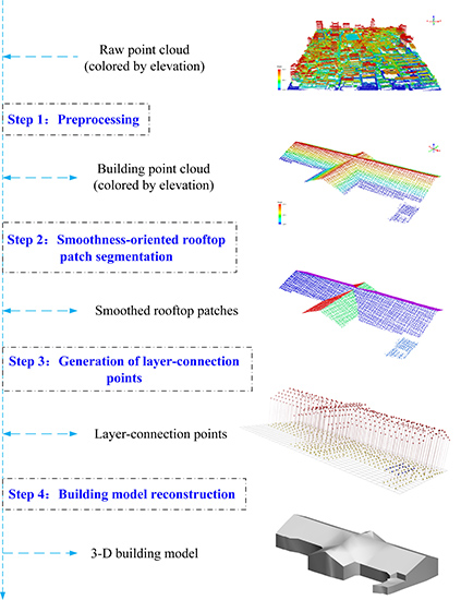
Rooftop patch optimization involves (1) smoothing of the rooftop patch points and (2) eliminating the interference of omissive LiDAR points.
The red box in
Figure 1a contains a number of protuberant points (
i.e., a small number of points above a large rooftop patch); however, these protuberant points were not seen in the rooftop patch segmentation results (
Figure 1b). If these protuberant points are directly discarded before building roof reconstruction, some holes will appear on the building roofs. As these points are usually distributed above the real rooftop patches, we set a distance threshold (2 m) to recognize them. After all the protuberant points have been found, they are projected to the corresponding segmented rooftop patch by using the plane equation calculated by the RANSAC algorithm [
29].
Furthermore, even if such points belong to the same rooftop patch, they may not be precisely distributed on the same plane. Hence, a smoothing operation must be conducted prior to the building roofs being reconstructed. Here, for each segmented rooftop patch, the RANSAC algorithm was applied to fit a virtual plane from the candidate points, and then the points were forced to move on to this estimated plane in order to assign a perfect flatness property to each surface. The smoothing procedures described above were conducted iteratively for all rooftop patches.
Figure 1c illustrates the point clouds after smoothing.
2.3. Generation of Layer-Connection Points
According to the derived rooftop patches, contour-based approaches are usually used for the reconstruction of 3-D building roofs. However, some major flaws impede the use of 3-D contours in building model reconstruction. These limitations are as follows: (1) the fitting of 3-D contours is strongly affected by noise; (2) the extraction of 3-D contours demands a large number of points, so the 3-D contours may be broken when not enough points are provided; and (3) the topological relationships of 3-D contours among different roof layers are difficult to confirm.
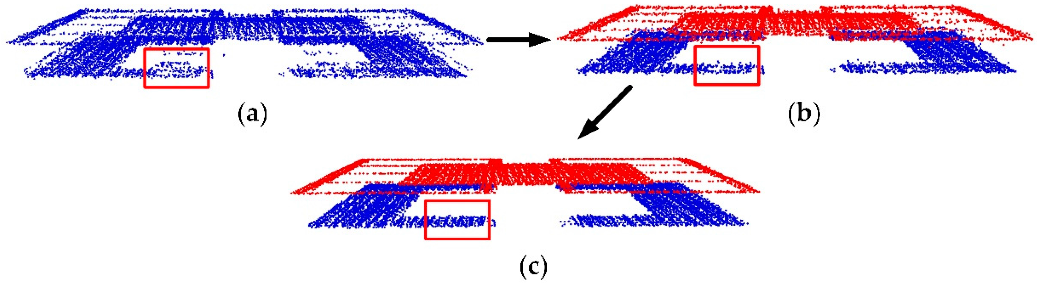
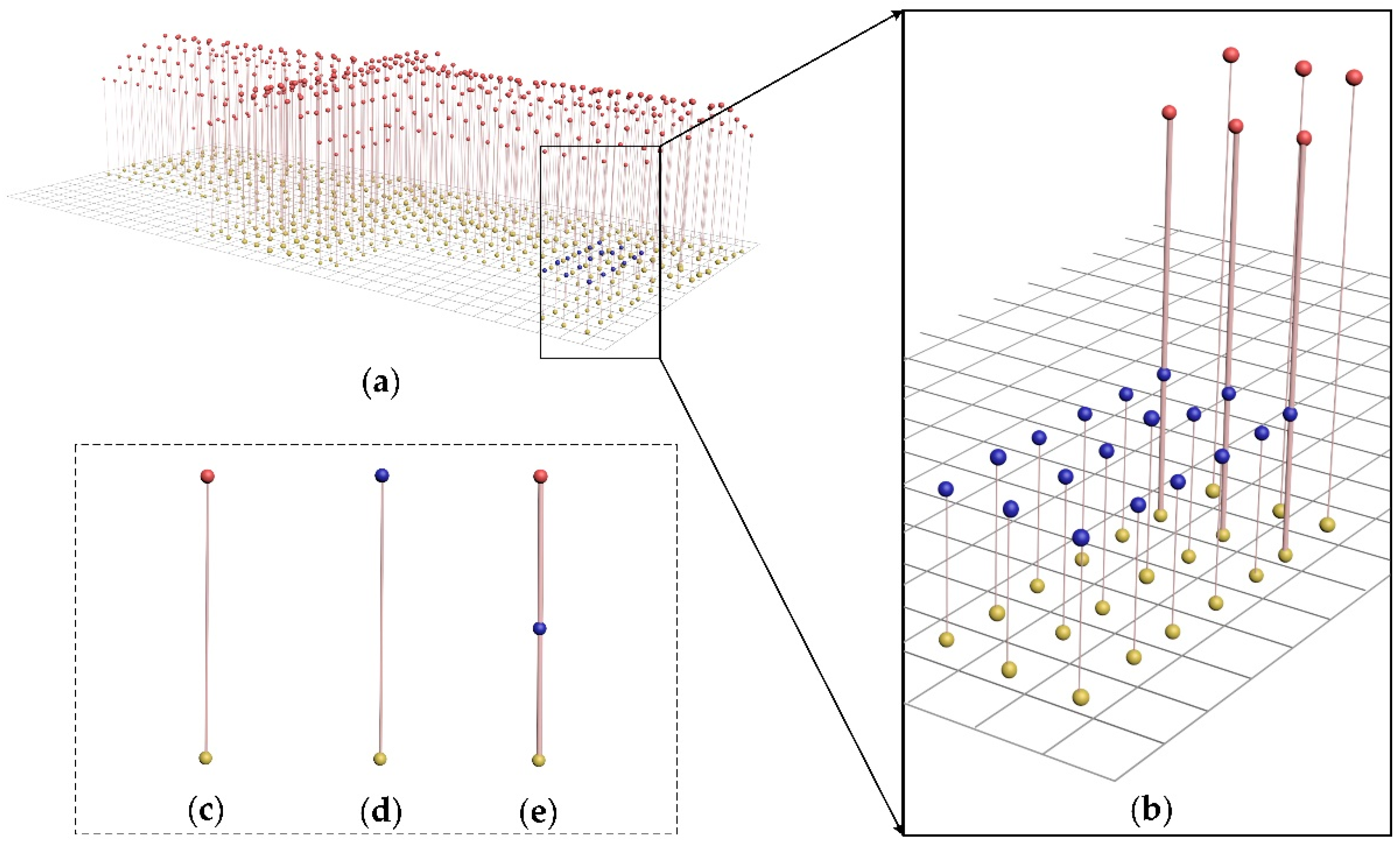
Therefore, a point-based method for 3-D building roof reconstruction is proposed here. The core objective of this method is to generate points to represent and connect roof layers (see
Figure 2), which are named as layer-connection points, for a building rooftop. Layer-connection points have two purposes, namely, to represent a roof layer in the horizontal direction and to connect different roof layers in the vertical direction. In the horizontal direction, as shown in
Figure 2a,b, yellow points represent the first layer (ground), blue points represent the second layer, and red points represent the third layer. These points with different colors are defined as layer-points. In the vertical direction, as shown in
Figure 2c, a yellow point and red point form a line to connect the corresponding local region of the first layer and the third layer. These two layer-points, which have the same
x–
y coordinates but different
z values, as a whole, are called a layer-connection point. Similarly, in
Figure 2d, a yellow point and blue point form a line to connect the first layer and the second layer. Moreover, in
Figure 2e, a yellow point, blue point, and red point form a line to connect the first layer, the second layer, and the third layer. These three layer-points, as a whole, are also called a layer-connection point.
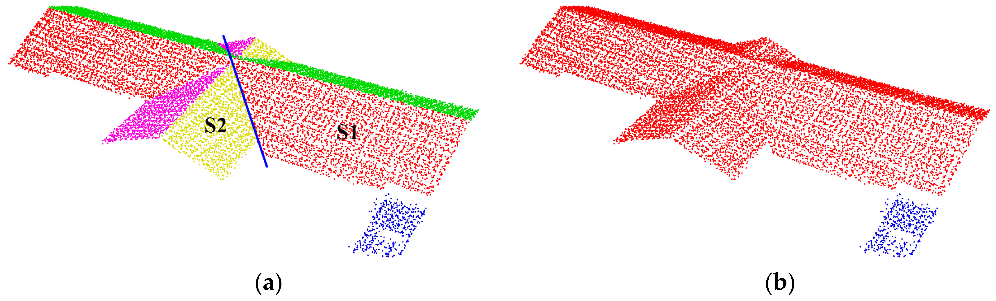
Before calculation of layer-connection points, we need to merge the rooftop patches into several roof layers. First, we give a clear definition of the
roof layer. A roof layer is defined as being made up of several rooftop patches, which are adjacent and intersected with one another. For example, in
Figure 2a, the red points represent the third layer, but the layer has four different rooftop patches, and, therefore, the four rooftop patches should be merged into a roof layer. Airborne LiDAR points corresponding to different rooftop patches are used as source data for merging. Here, we first introduce the principles for merging rooftop patches. The principles include whether there is an intersection line and an adjacent relationship between two rooftop patches. For example, in
Figure 3a, there are two rooftop patches,
i.e.,
S1 (red points in
Figure 3a) and
S2 (yellow points in
Figure 3a). When
S1 and
S2 have an intersection line (blue line in
Figure 3a), and the two rooftop patches have an adjacent relationship, they can be merged into the same roof layer. After the completion of judgments for all rooftop patches in accordance with the above principles, we can obtain the final merging results, as illustrated in
Figure 3b. After the merging of rooftop patches, the layer-connection points can be calculated.
2.3.1. Construction of the 2-D Grid System
Before calculating the layer-connection points, we need to create a 2-D grid system. Thus, the scale and grid cell size of the 2-D grid system need to be determined. The scale of the grid system is set according to the maximum and minimum values of the point clouds in the
X and
Y directions. To guarantee that a reasonable number of points lie inside each grid cell, the grid cell size is set to 2–3 times the average point spacing (we set it to 1.0 m in this study). The grid cells record the serial numbers of each LiDAR point within them, and a cell with no points is said to be empty. For each LiDAR point, we record the row and column number of its corresponding cell to construct a two-way index. The index of a point with coordinates (
x,
y,
z) can be obtained from the following formula:
where
i and
j represent the number of row and column of a grid cell, respectively, (
xmin,
ymin) represents the minimum coordinates of the building points, and
Gridsize represents the size of a grid cell.
2.3.2. Calculation of Layer-Connection Points
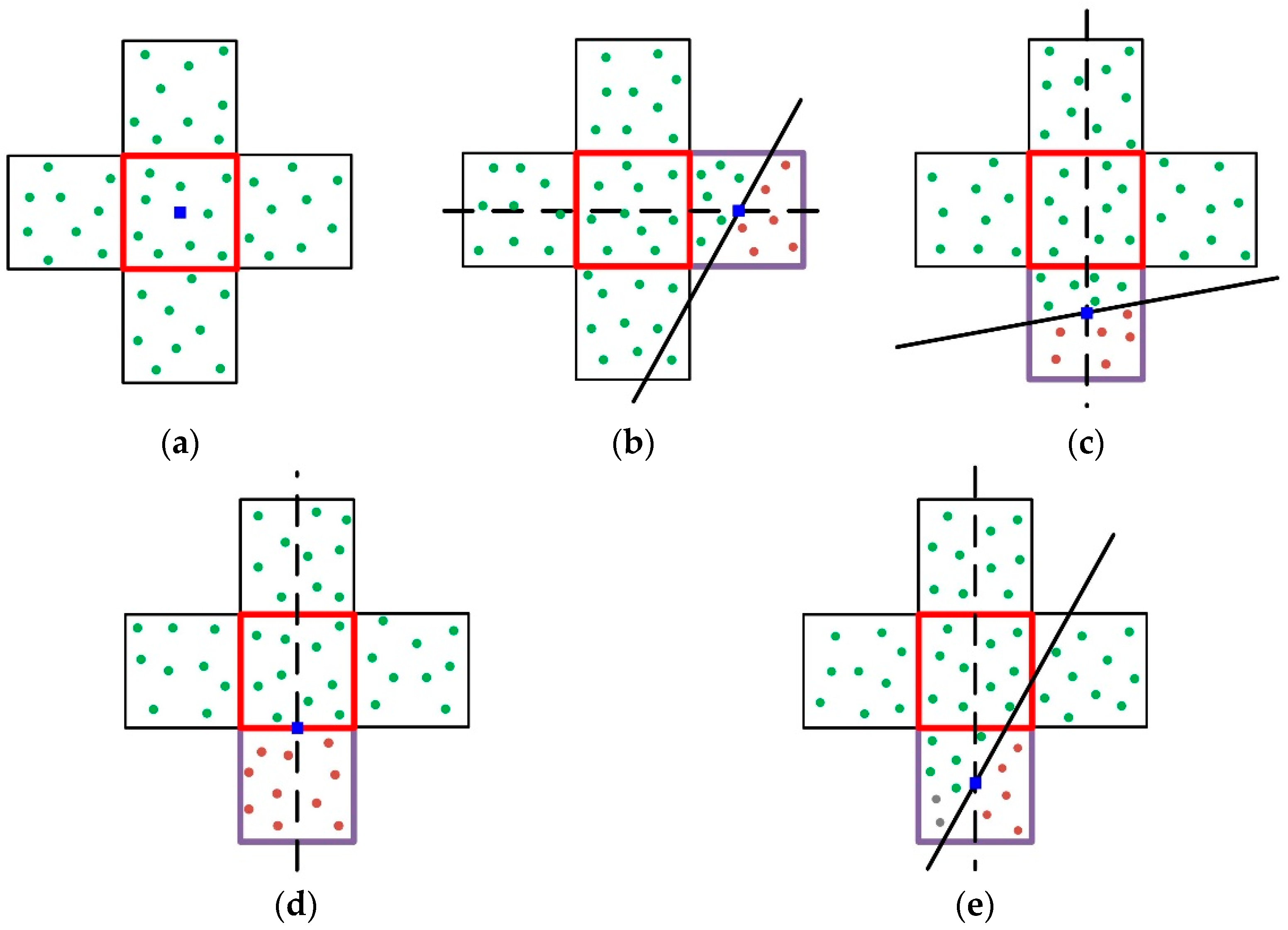
During the calculation of layer-connection points, a center cell and its neighboring four cells are taken into consideration. Aforementioned layer results are used to determine whether the LiDAR points in the neighboring four cells are on the same roof layer with that in the center cell. There are five potential situations.
In the first situation, as illustrated in
Figure 4a, where all LiDAR points belong to the same roof layer, the center cell (red box in
Figure 4a) does not contain any connections between different roof layers. In this situation, the cell will only generate a layer-point for the layer connection. The coordinates of this cell’s center (blue rectangle in
Figure 4a) are set as the
x–
y coordinates of this layer-point, and the average height value of all LiDAR points inside the center cell is set as its height.
In the second situation, as illustrated in
Figure 4b, where the LiDAR points inside the center cell and four neighboring cells do not belong to the same roof layer, the violet cell may contain connections between different roof layers. A line splitting different roof layers can be calculated on which a point to connect different layers can be located. If the cell (violet box in
Figure 4b) with LiDAR points from different roof layers lies to the left or right of the center cell (red box in
Figure 4b), a black dotted horizontal line is generated to intersect the splitting line (black solid line in
Figure 4b). The point of intersection (blue rectangle in
Figure 4b) is taken as the
x–
y coordinates of the layer-connection point. Simultaneously, the cell containing the planimetric coordinates of the intersection point is confirmed and the LiDAR points in it are selected. Based on these points, height values of each layer-point are determined by the average height of the LiDAR points of the corresponding roof layer.
In the third situation, as illustrated in
Figure 4c, if the cell (violet box in
Figure 4c) with LiDAR points from different roof layers lies above or below the center cell (red box in
Figure 4c), a black dotted vertical line is generated to intersect with the splitting line (black solid line in
Figure 4c). The point of intersection (blue rectangle in
Figure 4c) gives the
x–
y coordinates of the layer-connection point. Similarly, the cell containing the planimetric coordinates of the intersection point is confirmed and height values of each layer-point is determined by the average height of the LiDAR points of the corresponding roof layer.
In the fourth situation, as illustrated in
Figure 4d, if the
x–
y coordinates of the layer-connection point are exactly on the boundary of the center cell (red box in
Figure 4d), a black dotted vertical line intersecting the boundary gives the
x–
y coordinates of the layer-connection point (blue rectangle in
Figure 4d). Again, height values of each layer-point are set according to the average height value of the LiDAR points (red and violet cells) of the corresponding roof layer.
In the fifth situation, as illustrated in
Figure 4e, if the LiDAR points inside a cell (violet box in
Figure 4e) come from more than two roof layers, the number of points from each roof layer is counted, and only two major groups of points are used to determine the
x–
y coordinates. The subsequent calculations are the same as those used in situation two, three, or four.
2.3.3. Optimization of Layer-Connection Points
There are a number of layer-connection points distributed along building contours. If these layer-connection points are directly connected, a series of zigzag contours will be produced. Thus, the layer-connection points along building contours need to be smoothed. We applied Zhou’s method [
43], in which the principal orientations are derived from boundary points, and the points are iteratively fitted to a line running along the principal orientations.
2.4. Building Model Reconstruction
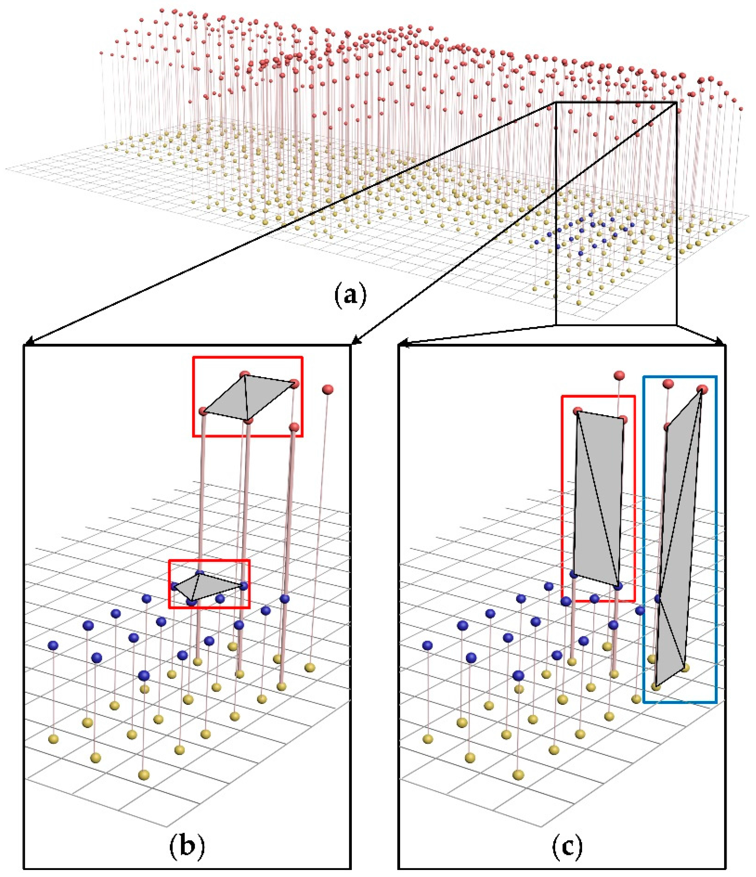
Figure 5a shows a sample of the layer-connection points generated by the proposed approach. As shown in
Figure 5a, a building model can be obtained by connecting neighboring layer-connection points.
For building roof reconstruction, the three neighboring cells should be searched, which correspond to three layer-connection points. If the layer-points of the layer-connection points inside the three neighboring cells are located on the same roof layer, these layer-points are connected to construct a triangle mesh (red box in
Figure 5b). By traversing all of the cells, the construction of rooftops can be completed.
This paper only focuses on building roof reconstruction. Therefore, building walls are replaced with vertical planes. A similar operation is performed to construct the building walls. Briefly, layer-connection points including multiple layer-points inside neighboring or diagonally adjacent cells indicate the existence of a building wall. By connecting the layer-points belonging to different roof layers (red box in
Figure 5c), this building wall can be obtained. In addition, the layer-connection points located on the boundary of a building must be connected to enable the construction of whole building walls (blue box in
Figure 5c).
2.5. Sensitivity Analysis of the Key Parameters
Given that a few parameters were used in this study, a summary of the setting procedures used for the associated key thresholds is necessary. The setting basis of these thresholds involved two types of information; namely, the data source and empirical results. The term “data source” means that a threshold is set according to the real data. If this method is applied to some other 3-D building model reconstruction, the “data source” thresholds can be determined easily, which increases the applicability of the proposed method. The term “empirical” means that the thresholds are set empirically, and in most cases, they can be set directly as we have proposed here.
During the process of extracting building rooftop points, the RIMM algorithm is employed. The parameters used during this step are shown in
Table 1. The initial window size
Iw and the height difference
Th were set according to the data source, and these values usually refer to the length of the largest building (106 m) and the height of the lowest building (3 m) in the experimental area, respectively. The fixed step length
Lc, and roughness value
Rv were, respectively, set to 3 m and 0.8 m, empirically. Two sets of different values (in meters) were tested while setting the values for the two parameters
Lc and
Rv. For
Lc the test values were 1, 3, 5, 7 m; for
Rv the test values were 0.4, 0.6, 0.8, 1.0, and 1.2 m. According to the completeness and correctness of the segmented rooftop patches, we found that the smaller
Lc and the larger
Rv could lead to that the extracted building point clouds contained some tree LiDAR points. Conversely, there could be some missing building points if
Lc was too large and
Rv was too small. The optimal extraction results were observed at
Lc = 3 m and
Rv = 0.8 m.
In the process of smoothness-oriented rooftop patch segmentation, an extraction method based on region growth and rooftop patch optimization is used. The key parameters are shown in
Table 1. As we can see, all parameters used in this step can be set empirically. The search radius
Rs and the number of inner points
N are related to the input LiDAR data. To guarantee that there were more than ten points to calculate the normal of each LiDAR point,
Rs is suitable for 2–3 times average of point spacing. Elaborate consideration was given to the value of
N as follows. We assumed that the area of a minimum rooftop patch that could be detected was 4 m
2,
i.e., 2 m × 2 m. According to the point density of LiDAR data, a threshold for
N can then be calculated easily. The distance threshold
Td were set to 0.2, 0.3, 0.4, 0.5, and 0.6 m to find the optimal value. In the process of patch optimization, the phenomenon of over-smoothing will be occurred, if
Td is set too large. At
Td = 0.5 m the effect of smoothing is moderate. The probability is a minimum probability of finding at least one good set of observations in all iterative procedures. It usually lies between 0.90 and 0.99. In our experiments, the probability was set to 0.98. During the generation of layer-connection points, a grid-based method is introduced, and the cell size is set empirically.
4. Conclusions
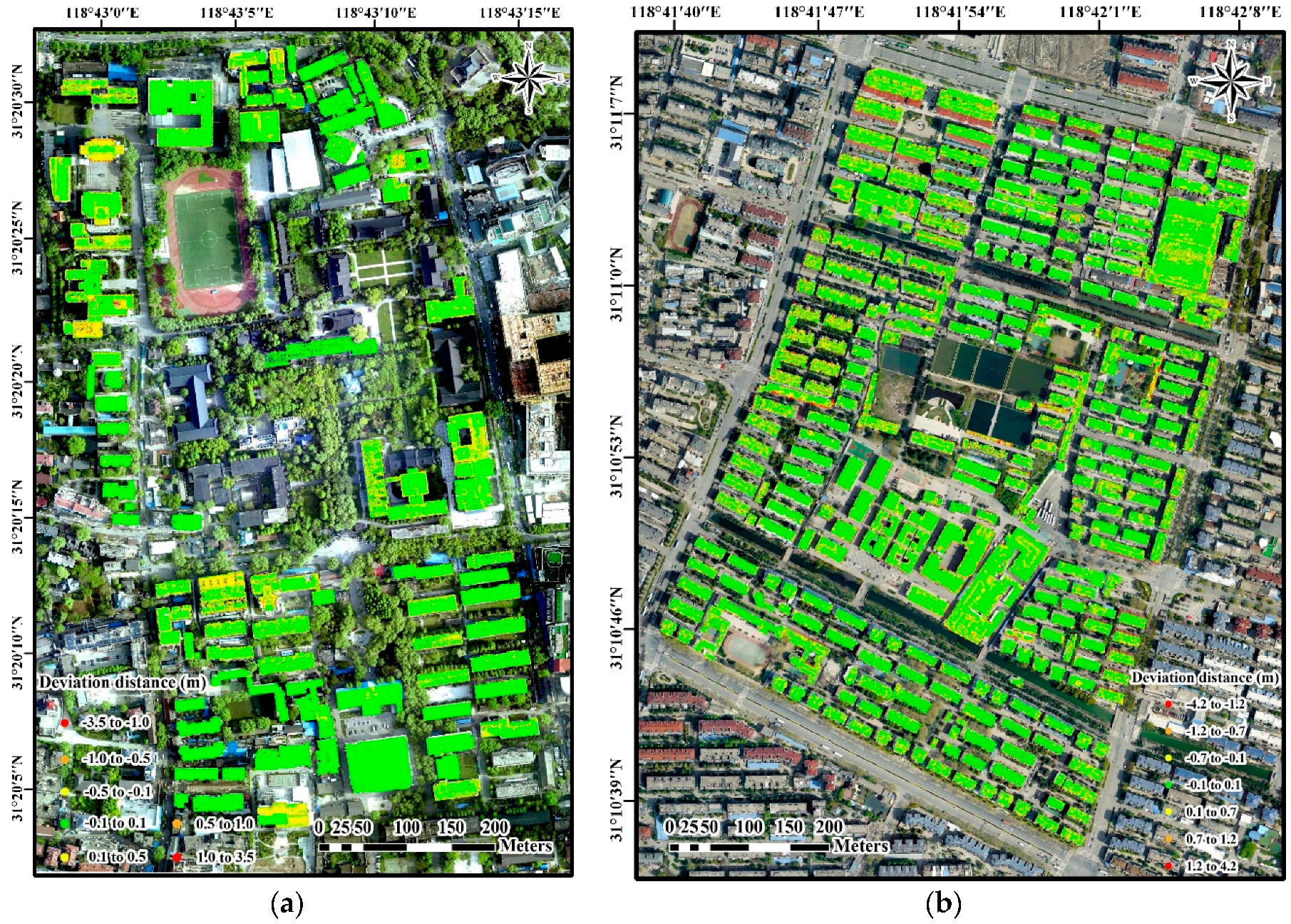
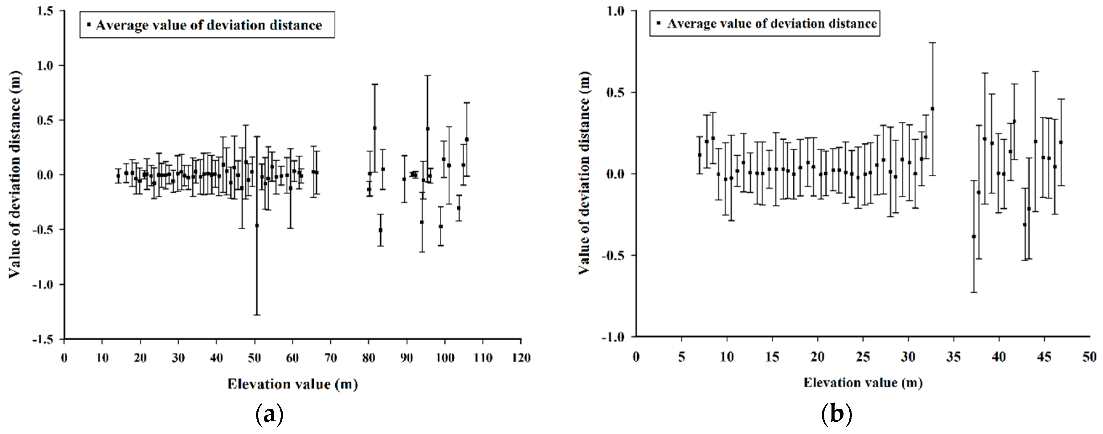
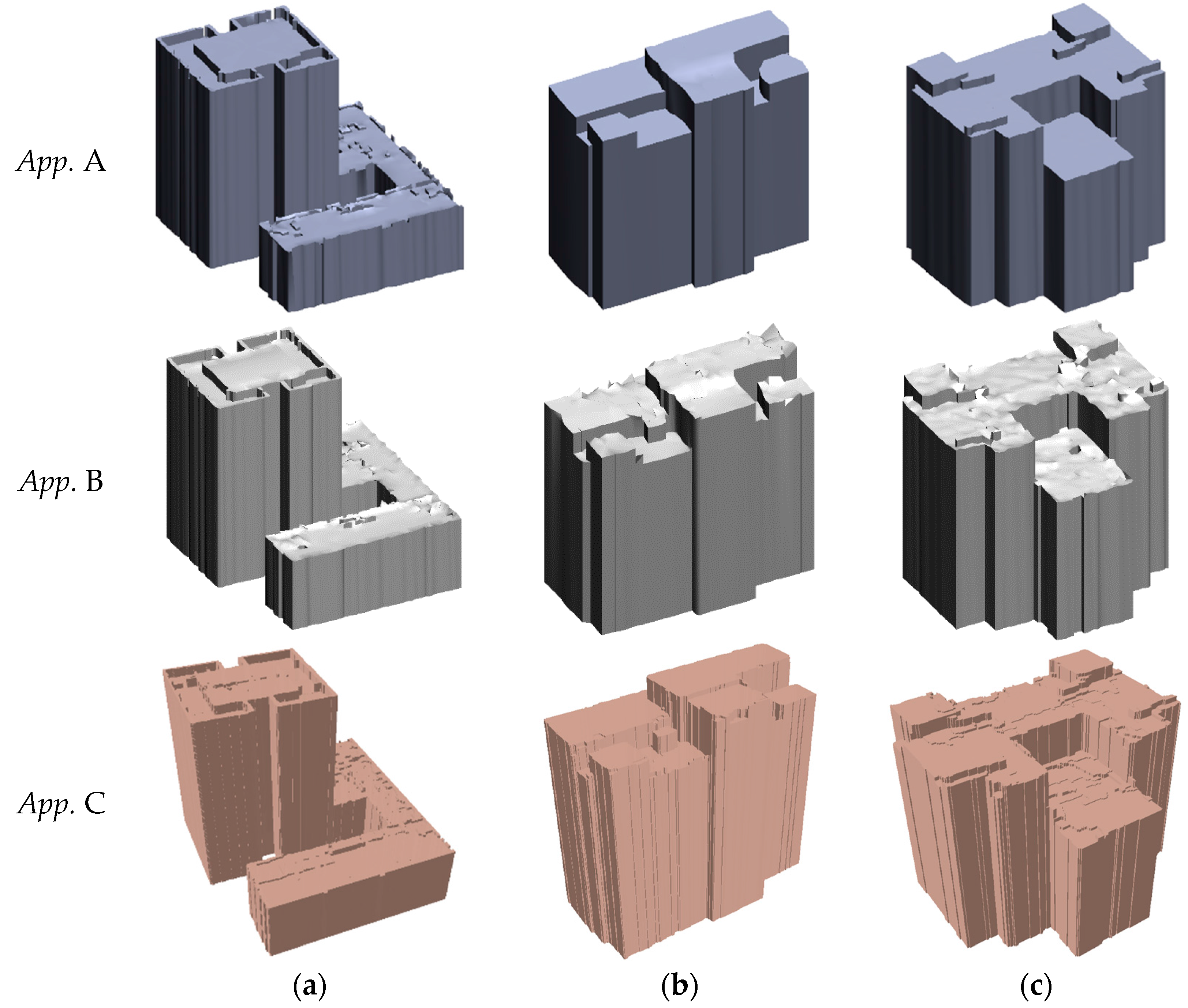
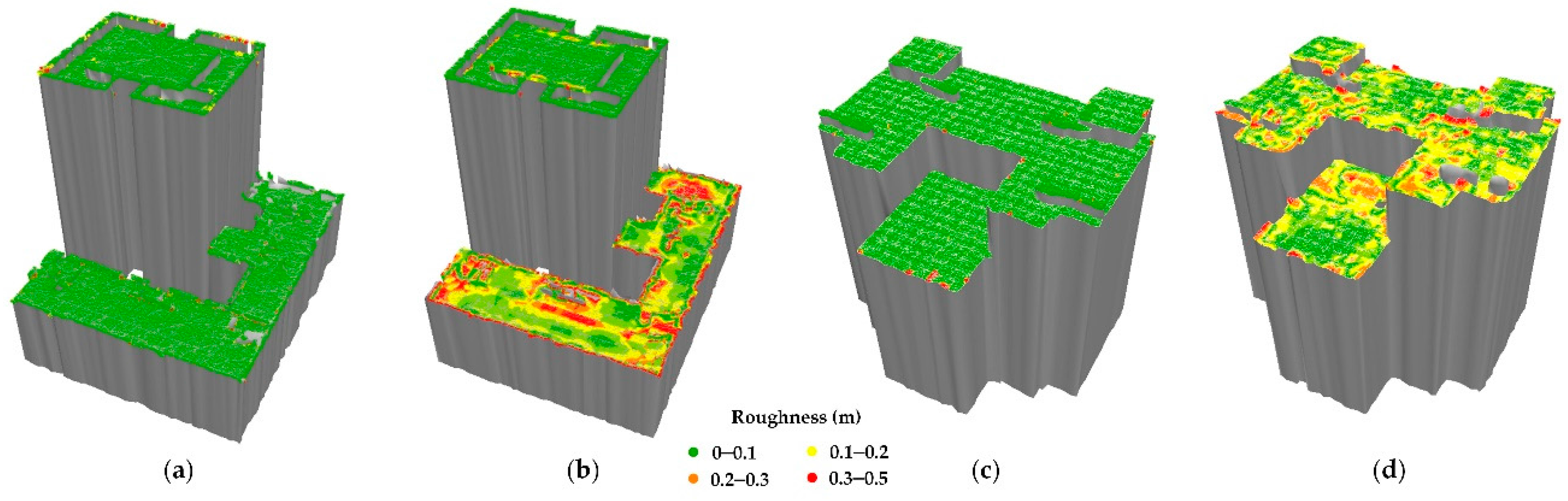
This paper has presented a new approach involving a layer connection and smoothness strategy for the reconstruction of building roof models from airborne LiDAR data. The proposed approach consists of building rooftop point extraction, smoothness-oriented rooftop patch extraction, layer-connection point generation, and building model reconstruction. The main contributions of the proposed approach are as follows. (1) During the rooftop patch extraction, a “seed point selection, patch growth, and patch smoothing” strategy is used to smooth building points, eliminate interference information, and ensure the integrity of the point cloud data; and (2) layer-connection points are proposed to guarantee consistency between the boundary footprints of different roof layers. By connecting neighboring layer-connection points, the building roofs are reconstructed. Through the calculation of layer-connection points, different roof layers are connected in a simple and fast way. In the two experimental regions used in this paper, the completeness and correctness of the reconstructed rooftop patches were about 90% and 95%, respectively. For the deviation accuracy, the average deviation distance and standard deviation in the best case were 0.05 m and 0.18 m, respectively, and those in the worst case were 0.12 m and 0.25 m. Our experiments prove that this method has good applicability for model reconstruction of buildings in urban environments.
However, too many types of geometric shapes may exist on building roofs, such as artistic sculptures, curved surfaces, and so forth. Therefore, there could be some phenomena of over-smoothing for not-flat roofs by using the proposed method. To reconstruct building roofs with very complex structures, further investigations will be necessary. In addition, small mistakes can persist in certain tiny structures such as fences, air conditioning vents, and chimneys. The proposed method cannot deal with roof overhangs, which are also difficult to reconstruct by the most previous methods. In our future work, we will consider to reconstruct these roof parts with the aid of the auxiliary data (e.g., terrestrial LiDAR data). This paper has concentrated on the reconstruction of building roofs from airborne LiDAR data, and little work was done for the subtle reconstruction of building façades. To achieve the reconstruction of complete building models, further work is needed to allow for the subtle reconstruction of façade models from terrestrial LiDAR data.


 and
and 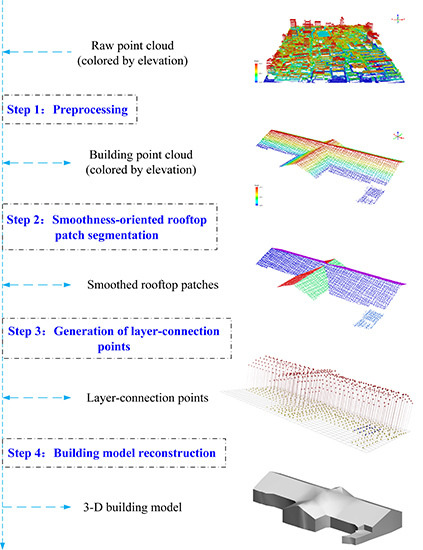


