
Building Point Detection from Vehicle-Borne LiDAR Data Based on Voxel Group and Horizontal Hollow Analysis

Abstract
:
1. Introduction
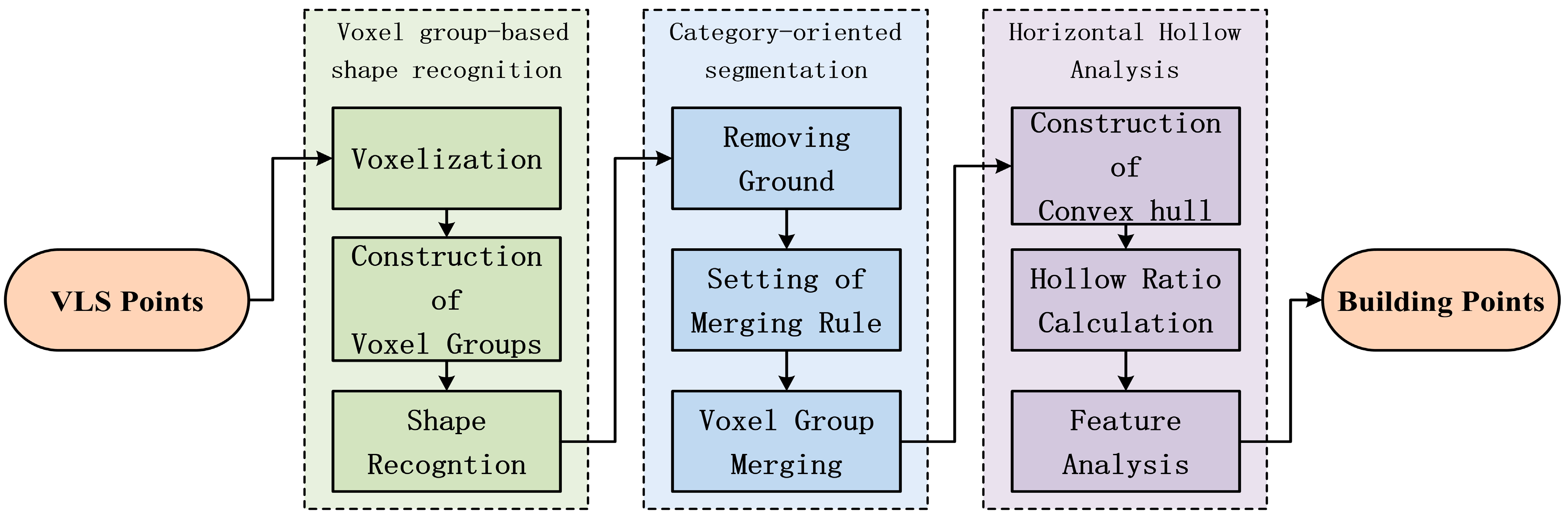
2. Methods
2.1. Voxel Group-Based Shape Recognition
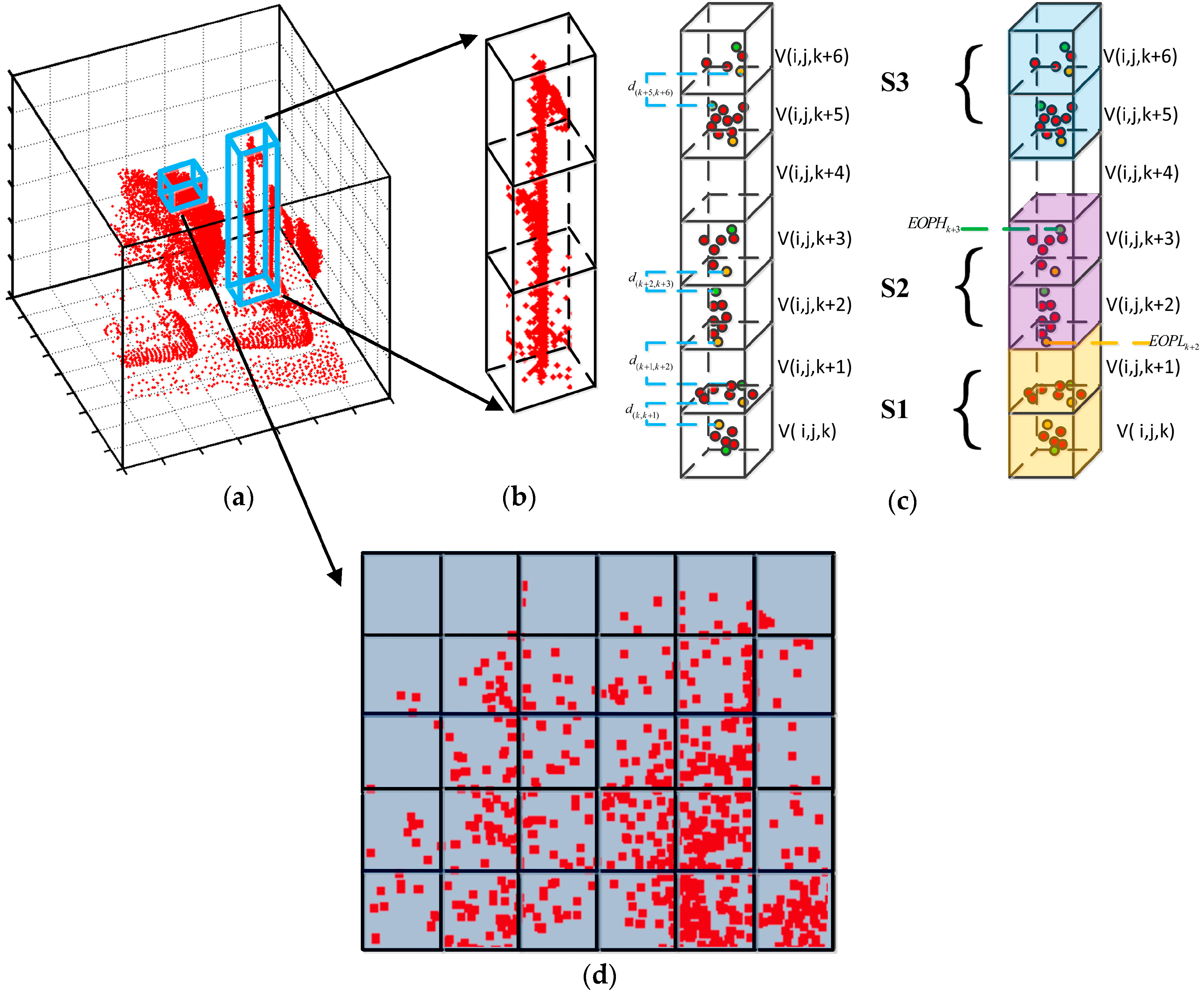
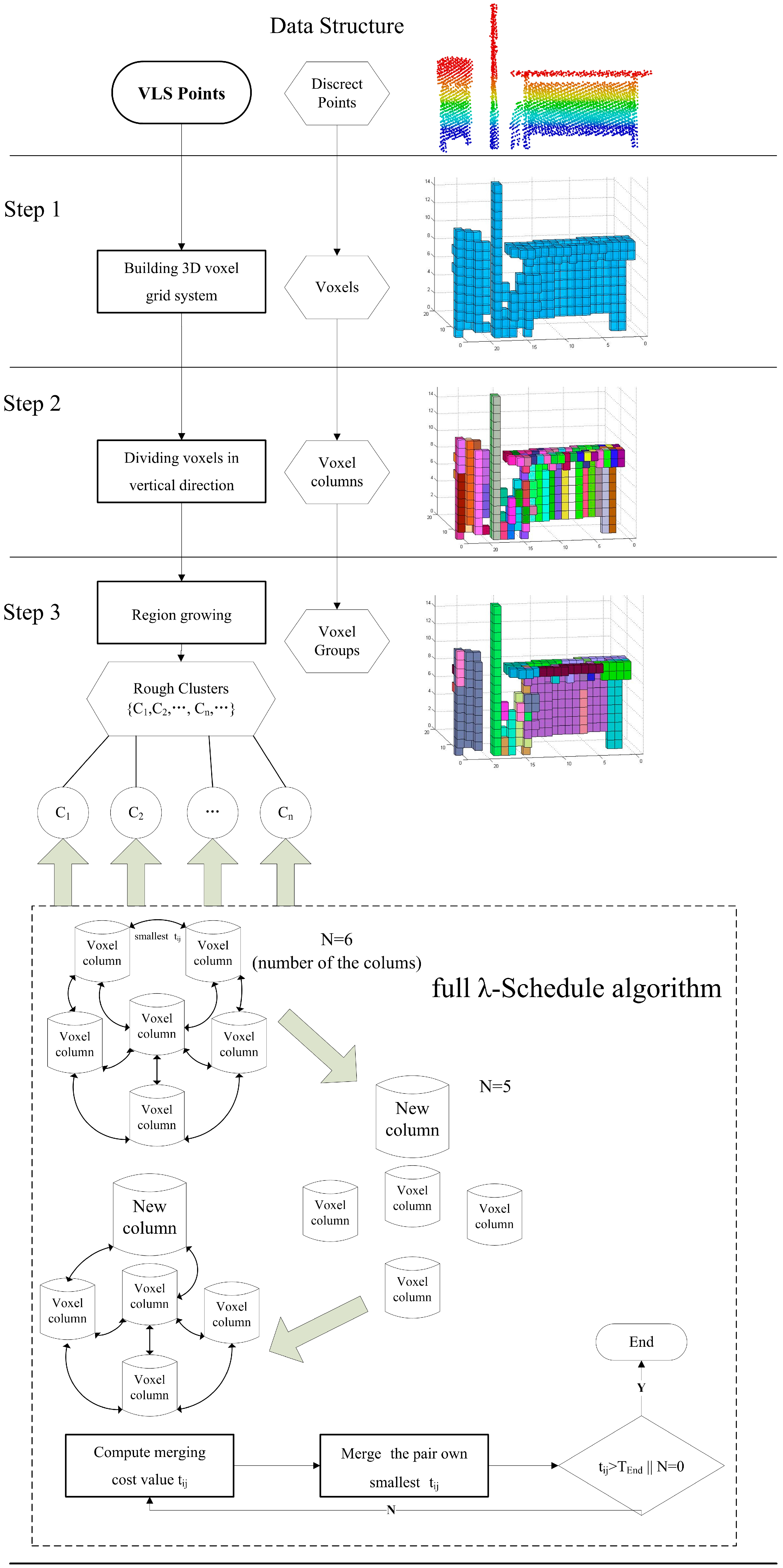
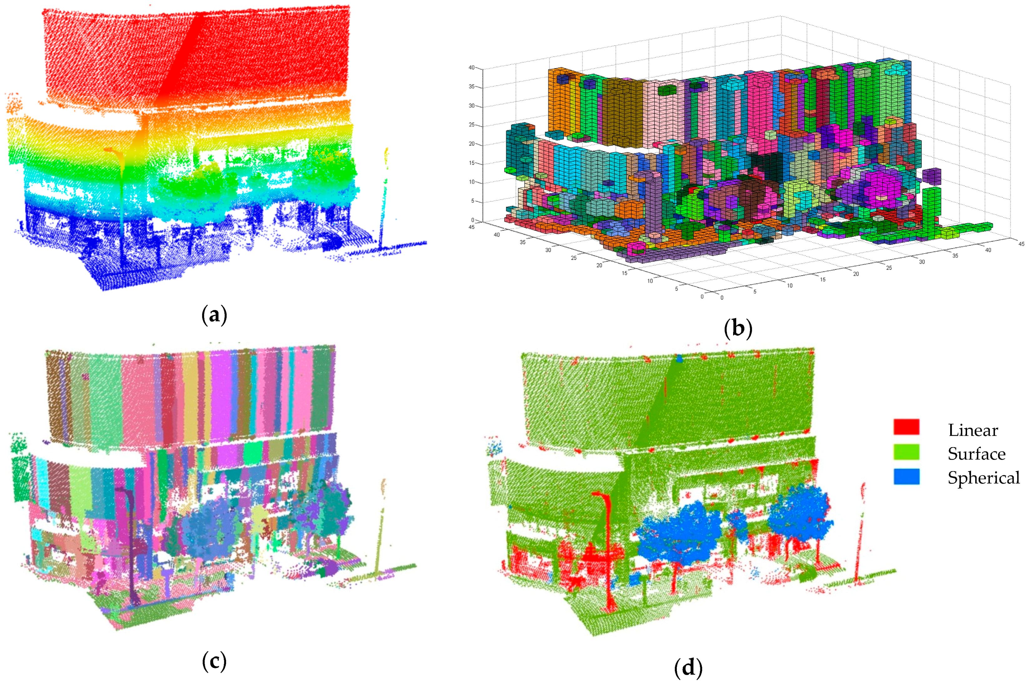
2.1.1. Voxelization
2.1.2. Generating of Voxel Group
- Take a simple region growth for whole voxel columns in horizontal direction based on connectivity to get several rough clusters: .
- Compute all the pairs of adjacent voxel columns within Cn and their merging cost value from Equation (6) and sort them into a list.
- Merge the pair (Si,Sj) which own smallest ti,j to form a new voxel column Sij and update the merging cost value.
- Repeat the step ii and step iii until the ti,j exceeds the threshold TEnd or all the voxel columns within Cn into one group.
- Repeat the step ii, iii, iv until all clusters are processed.
2.1.3. Shape Recognition of Each Voxel Group
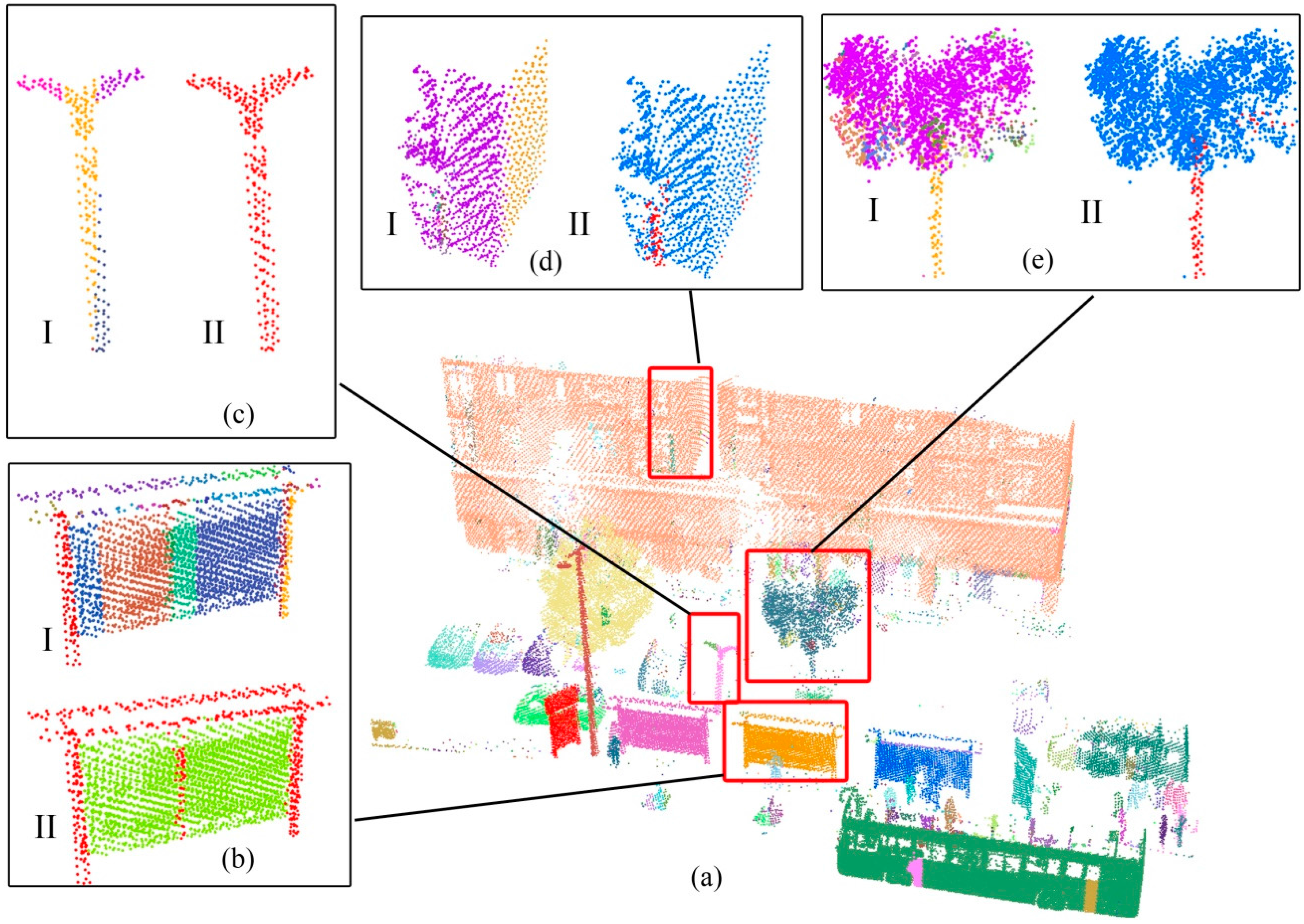
2.2. Category-Oriented Merging
2.2.1. Removing Ground Points
2.2.2. Category-Oriented Merging
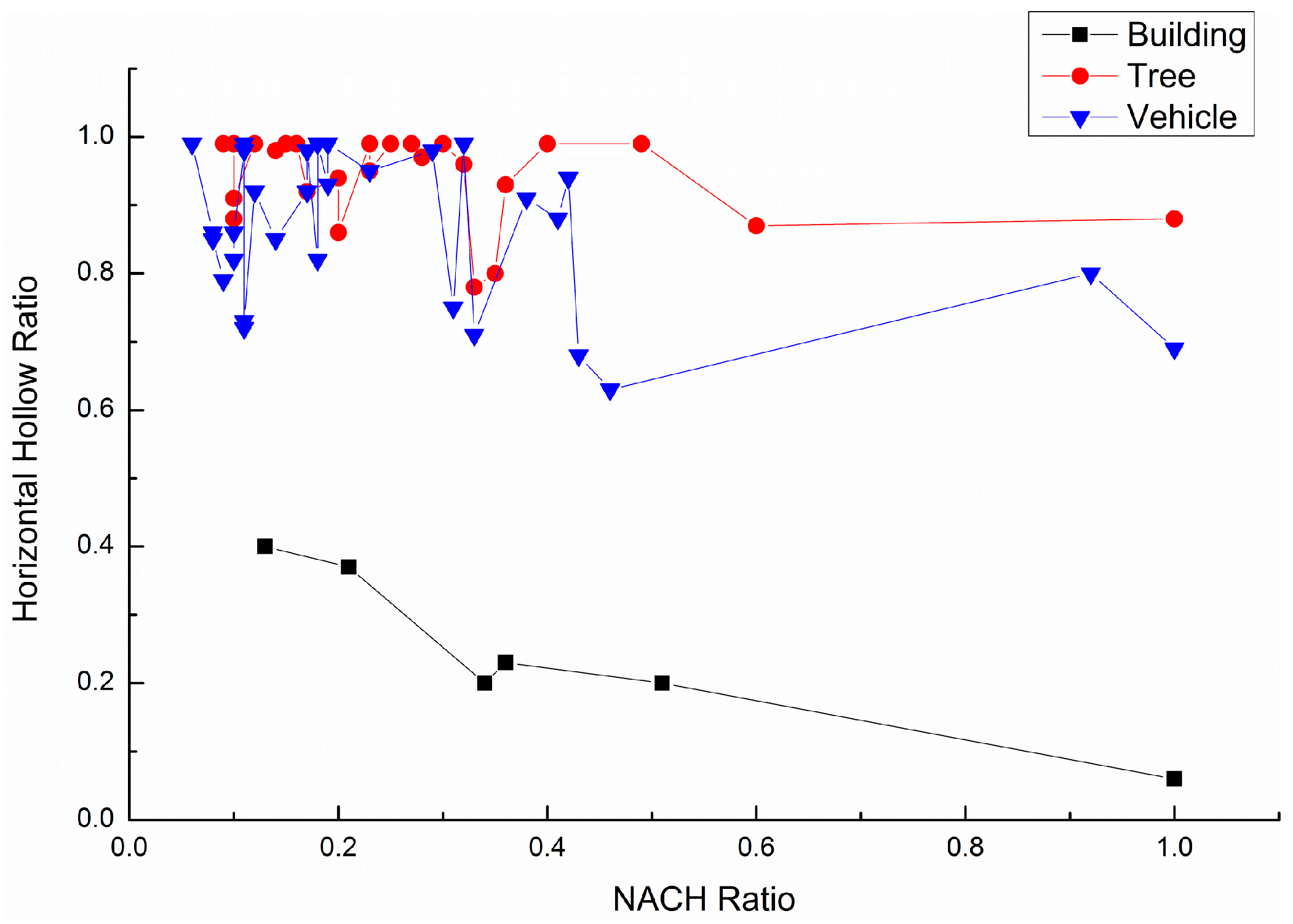
2.3. Horizontal Hollow Ratio-Based Building Point Identification
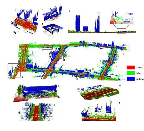
3. Results and Discussion
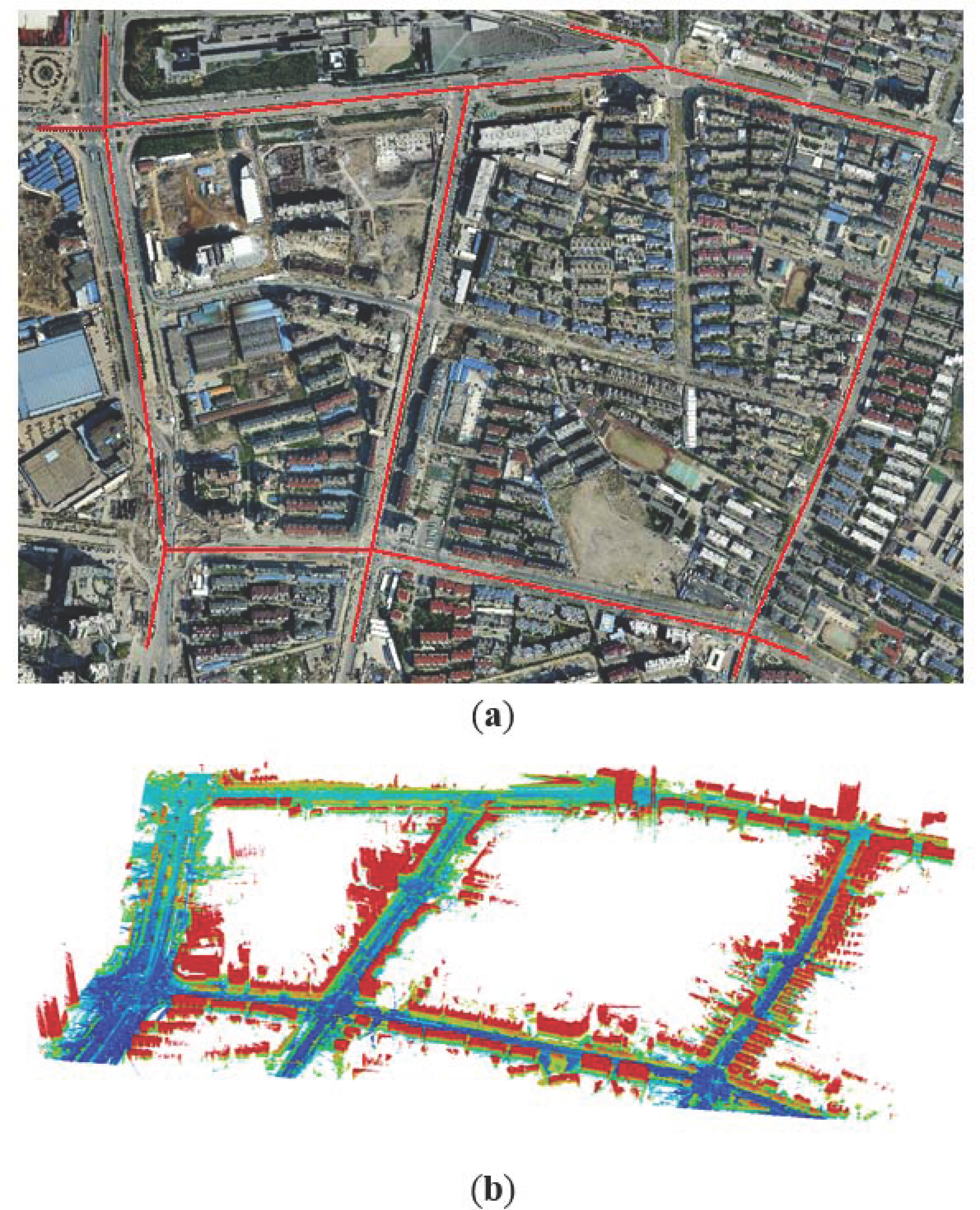
3.1. Study Area and Experimental Data
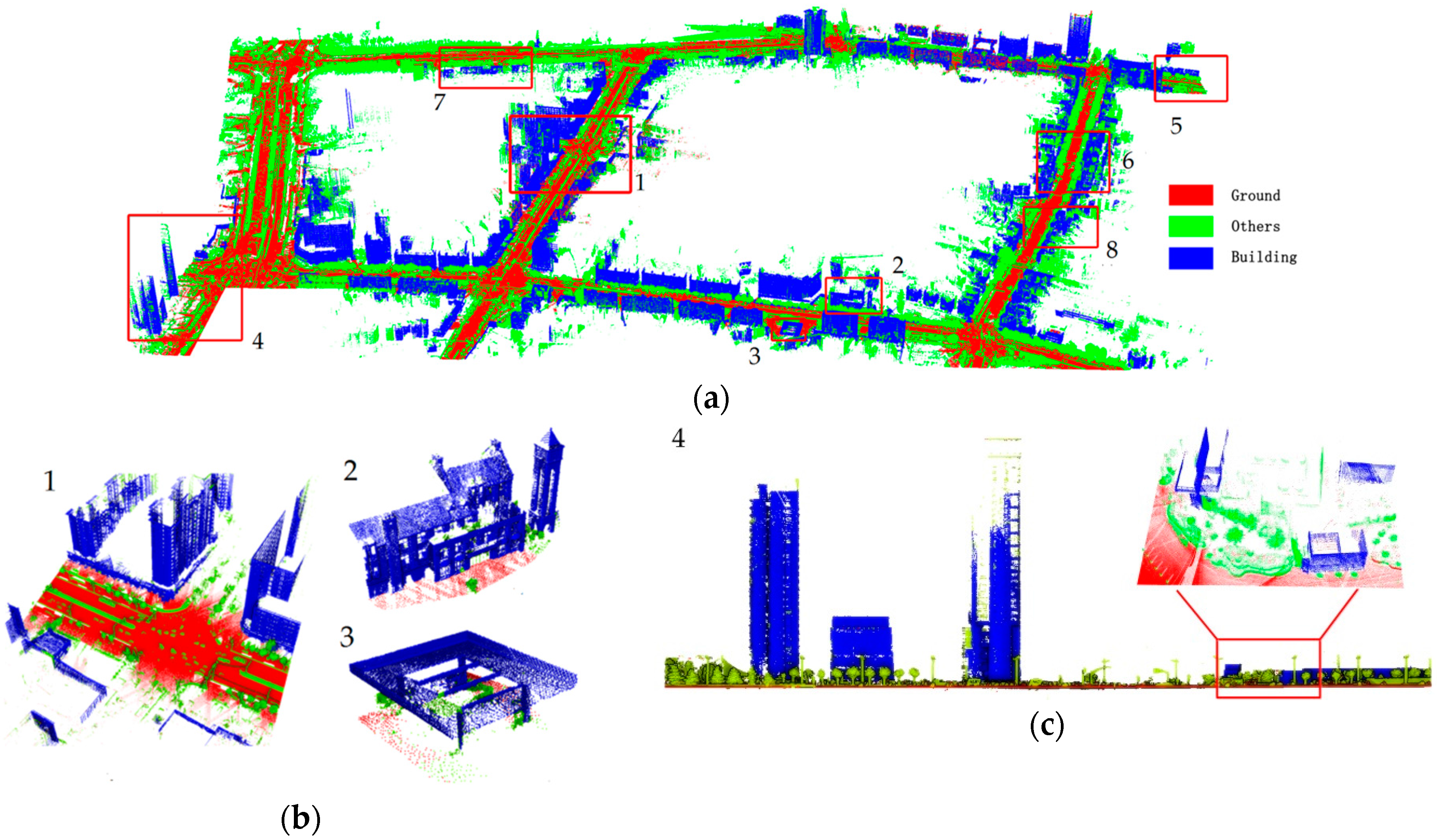
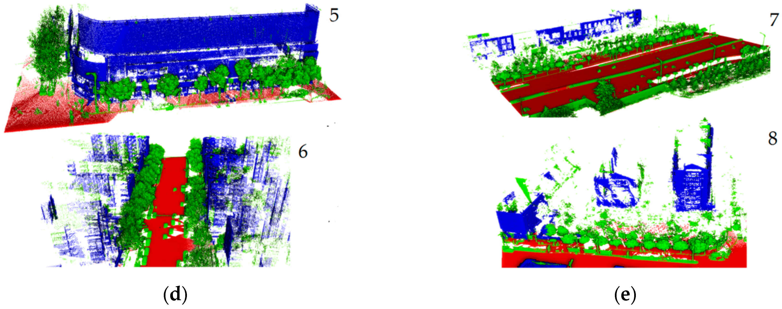
3.2. Extraction Results of Building Points
3.3. Evaluation of Extraction Accuracy
3.3.1. Building-Based Evaluation for Overall Experimental Area
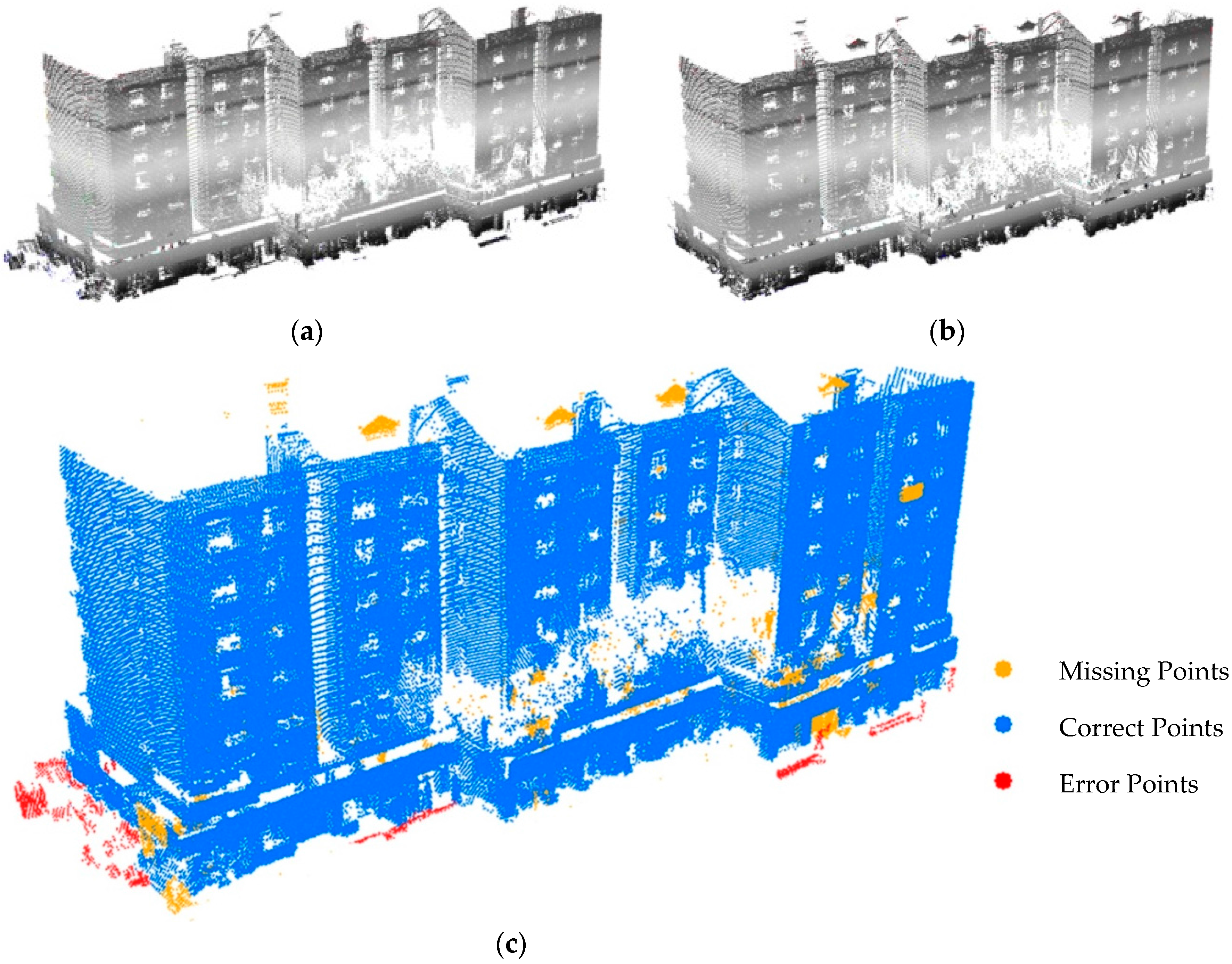
3.3.2. Point-Based Evaluation for Individual Building
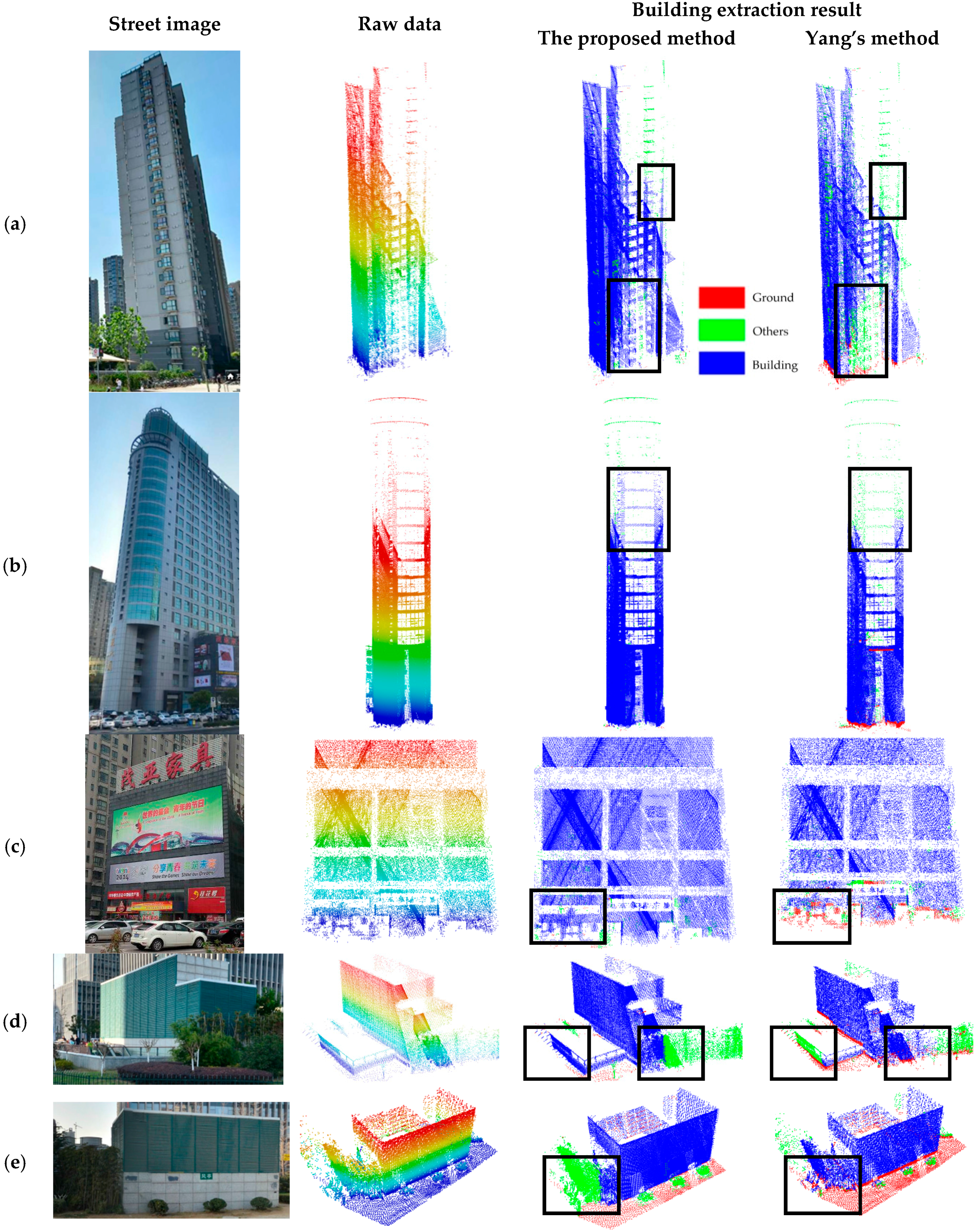
3.4. Experiment Discussion
4. Conclusions
Acknowledgments
Author Contributions
Conflicts of Interest
Abbreviations
| MDPI | Multidisciplinary Digital Publishing Institute |
| DOAJ | Directory of open access journals |
| TLA | Three letter acronym |
| LD | linear dichroism |
References
- Yang, B.; Wei, Z.; Li, Q.; Li, J. Semiautomated building facade footprint extraction from mobile LiDAR point clouds. IEEE Geosci. Remote Sens. Lett. 2013, 10, 766–770. [Google Scholar] [CrossRef]
- Hong, S.; Jung, J.; Kim, S.; Cho, H.; Lee, J.; Heo, J. Semi-automated approach to indoor mapping for 3D as-built building information modeling. Comput. Environ. Urban Syst. 2015, 51, 34–46. [Google Scholar] [CrossRef]
- Remondino, F. Heritage recording and 3D modeling with photogrammetry and 3D scanning. Remote Sens. 2011, 3, 1104–1138. [Google Scholar] [CrossRef] [Green Version]
- Cheng, L.; Wang, Y.; Chen, Y.; Li, M. Using LiDAR for digital documentation of ancient city walls. J. Cult. Herit. 2016, 17, 188–193. [Google Scholar] [CrossRef]
- He, M.; Zhu, Q.; Du, Z.; Hu, H.; Ding, Y.; Chen, M. A 3D shape descriptor based on contour clusters for damaged roof detection using airborne LiDAR point clouds. Remote Sens. 2016, 8, 189. [Google Scholar] [CrossRef]
- Cheng, L.; Gong, J.; Li, M.; Liu, Y. 3D building model reconstruction from multi-view aerial imagery and LiDAR data. Photogramm. Eng. Remote Sens. 2011, 77, 125–139. [Google Scholar] [CrossRef]
- Wu, B.; Yu, B.; Yue, W.; Shu, S.; Tan, W.; Hu, C.; Huang, Y.; Wu, J.; Liu, H. A voxel-based method for automated identification and morphological parameters estimation of individual street trees from mobile laser scanning data. Remote Sens. 2013, 5, 584–611. [Google Scholar] [CrossRef]
- Rutzinger, M.; Rottensteiner, F.; Pfeifer, N. A comparison of evaluation techniques for building extraction from airborne laser scanning. IEEE J. Sel. Topics Appl. Earth Observ. Remote. 2009, 2, 11–20. [Google Scholar] [CrossRef]
- Sampath, A.; Shan, J. Segmentation and reconstruction of polyhedral building roofs from aerial LiDAR point clouds. IEEE Trans. Geosci. Remote Sens. 2010, 48, 1554–1567. [Google Scholar] [CrossRef]
- Kim, K.; Shan, J. Building roof modeling from airborne laser scanning data based on level set approach. ISPRS J. Photogramm. Remote Sens. 2011, 66, 484–497. [Google Scholar] [CrossRef]
- Yanming, C.; Liang, C.; Manchun, L.; Jiechen, W.; Lihua, T.; Kang, Y. Multiscale grid method for detection and reconstruction of building roofs from airborne LiDAR data. IEEE J. Sel. Topics Appl. Earth Observ. Remote Sens. 2014, 7, 4081–4094. [Google Scholar]
- Sun, S.; Salvaggio, C. Aerial 3D building detection and modeling from airborne LiDAR point clouds. IEEE J. Sel. Topics Appl. Earth Observ. Remote. 2013, 56, 1440–1449. [Google Scholar] [CrossRef]
- Rottensteiner, F. Automatic generation of high-quality building models from LiDAR data. IEEE Comput. Graphics Appl. 2003, 23, 42–50. [Google Scholar] [CrossRef]
- Li, Q.; Chen, Z.; Hu, Q. A model-driven approach for 3D modeling of pylon from airborne LiDAR data. Remote Sens. 2015, 7, 11501–11524. [Google Scholar] [CrossRef]
- Wang, R. 3D building modeling using images and LiDAR: A review. Int. J. Image Data Fusion 2013, 4, 273–292. [Google Scholar] [CrossRef]
- Xu, H.; Cheng, L.; Li, M.; Chen, Y.; Zhong, L. Using octrees to detect changes to buildings and trees in the urban environment from airborne LiDAR data. Remote Sens. 2015, 7, 9682–9704. [Google Scholar] [CrossRef]
- Xu, S.; Vosselman, G.; Oude Elberink, S. Detection and classification of changes in buildings from airborne laser scanning data. Remote Sens. 2015, 7, 17051–17076. [Google Scholar] [CrossRef]
- Pu, S.; Rutzinger, M.; Vosselman, G.; Oude Elberink, S. Recognizing basic structures from mobile laser scanning data for road inventory studies. ISPRS J. Photogramm. Remote Sens. 2011, 66, S28–S39. [Google Scholar] [CrossRef]
- Vo, A.V.; Truong-Hong, L.; Laefer, D.F. Aerial laser scanning and imagery data fusion for road detection in city scale. In Proceedings of the 2015 IEEE International Geoscience and Remote Sensing Symposium (IGARSS), Milan, Italy, 26–31 July 2015.
- Tong, L.; Cheng, L.; Li, M.; Wang, J.; Du, P. Integration of LiDAR data and orthophoto for automatic extraction of parking lot structure. IEEE J. Sel. Topics Appl. Earth Observ. Remote Sens. 2014, 7, 503–514. [Google Scholar] [CrossRef]
- Cheng, L.; Zhao, W.; Han, P.; Zhang, W.; Shan, J.; Liu, Y.; Li, M. Building region derivation from LiDAR data using a reversed iterative mathematic morphological algorithm. Opt. Commun. 2013, 286, 244–250. [Google Scholar] [CrossRef]
- Mongus, D.; Lukač, N.; Žalik, B. Ground and building extraction from LiDAR data based on differential morphological profiles and locally fitted surfaces. ISPRS J. Photogramm. Remote Sens. 2014, 93, 145–156. [Google Scholar] [CrossRef]
- Chun, L.; Beiqi, S.; Xuan, Y.; Nan, L.; Hangbin, W. Automatic buildings extraction from LiDAR data in urban area by neural oscillator network of visual cortex. IEEE J. Sel. Topics Appl. Earth Observ. Remote Sens. 2013, 6, 2008–2019. [Google Scholar]
- Berger, C.; Voltersen, M.; Hese, S.; Walde, I.; Schmullius, C. Robust extraction of urban land cover information from HSR multi-spectral and LiDAR data. IEEE J. Sel. Topics Appl. Earth Observ. Remote Sens. 2013, 6, 2196–2211. [Google Scholar] [CrossRef]
- Zhang, J.; Lin, X. Advances in fusion of optical imagery and LiDAR point cloud applied to photogrammetry and remote sensing. Int. J. Image Data Fusion 2016, 2016, 1–31. [Google Scholar] [CrossRef]
- Becker, S.; Haala, N. Grammar supported facade reconstruction from mobile LiDAR mapping. Int. Arch. Photogramm. Remote Sens. 2009, 38, 13–16. [Google Scholar]
- Chan, T.O.; Lichti, D.D.; Glennie, C.L. Multi-feature based boresight self-calibration of a terrestrial mobile mapping system. ISPRS J. Photogramm. Remote Sens. 2013, 82, 112–124. [Google Scholar] [CrossRef]
- Manandhar, D.; Shibasaki, R. Auto-extraction of urban features from vehicle-borne laser data. Int. Arch. Photogramm. Remote Sens. 2002, 34, 650–655. [Google Scholar]
- Hammoudi, K.; Dornaika, F.; Soheilian, B.; Paparoditis, N. Extracting outlined planar clusters of street facades from 3D point clouds. In Proceedings of the 2010 Canadian Conference on Computer and Robot Vision (CRV), Ottawa, ON, Canada, 31 May–2 June 2010.
- Jochem, A.; Höfle, B.; Rutzinger, M. Extraction of vertical walls from mobile laser scanning data for solar potential assessment. Remote Sens. 2011, 3, 650–667. [Google Scholar] [CrossRef]
- Tarsha-Kurdi, F.; Landes, T.; Grussenmeyer, P. Hough-transform and extended ransac algorithms for automatic detection of 3D building roof planes from LiDAR data. Proc. ISPRS 2007, 36, 407–412. [Google Scholar]
- Rutzinger, M.; Elberink, S.O.; Pu, S.; Vosselman, G. Automatic extraction of vertical walls from mobile and airborne laser scanning data. Int. Arch. Photogramm. Remote Sens. Spat. Inf. Sci. 2009, 38, W8. [Google Scholar]
- Moosmann, F.; Pink, O.; Stiller, C. Segmentation of 3D LiDAR data in non-flat urban environments using a local convexity criterion. In Proceedings of the 2009 IEEE Intelligent Vehicles Symposium, Xi’an, China, 3–5 June 2009.
- Munoz, D.; Vandapel, N.; Hebert, M. Directional associative markov network for 3D point cloud classification. In Proceedings of the Fourth International Symposium on 3D Data Processing, Visualization and Transmission, Atlanta, GA, USA, 18 June 2008.
- Demantké, J.; Mallet, C.; David, N.; Vallet, B. Dimensionality based scale selection in 3D LiDAR point clouds. Proc. ISPRS 2011, 38, W52. [Google Scholar] [CrossRef]
- Yang, B.; Dong, Z. A shape-based segmentation method for mobile laser scanning point clouds. ISPRS J. Photogramm. Remote Sens. 2013, 81, 19–30. [Google Scholar] [CrossRef]
- Yang, B.; Dong, Z.; Zhao, G.; Dai, W. Hierarchical extraction of urban objects from mobile laser scanning data. ISPRS J. Photogramm. Remote Sens. 2015, 99, 45–57. [Google Scholar] [CrossRef]
- Li, B.; Li, Q.; Shi, W.; Wu, F. Feature extraction and modeling of urban building from vehicle-borne laser scanning data. Proc. ISPRS 2004, 35, 934–939. [Google Scholar]
- Aijazi, A.K.; Checchin, P.; Trassoudaine, L. Segmentation based classification of 3D urban point clouds: A super-voxel based approach with evaluation. Remote Sens. 2013, 5, 1624–1650. [Google Scholar] [CrossRef]
- Yang, B.; Wei, Z.; Li, Q.; Li, J. Automated extraction of street-scene objects from mobile LiDAR point clouds. Int. J. Remote Sens. 2012, 33, 5839–5861. [Google Scholar] [CrossRef]
- Truong-Hong, L.; Laefer, D.F. Quantitative evaluation strategies for urban 3D model generation from remote sensing data. Comput. Graphics 2015, 49, 82–91. [Google Scholar] [CrossRef]
- Weishampel, J.F.; Blair, J.; Knox, R.; Dubayah, R.; Clark, D. Volumetric LiDAR return patterns from an old-growth tropical rainforest canopy. Int. J. Remote Sens. 2000, 21, 409–415. [Google Scholar] [CrossRef]
- Riano, D.; Meier, E.; Allgöwer, B.; Chuvieco, E.; Ustin, S.L. Modeling airborne laser scanning data for the spatial generation of critical forest parameters in fire behavior modeling. Remote Sens. Environ. 2003, 86, 177–186. [Google Scholar] [CrossRef]
- Chasmer, L.; Hopkinson, C.; Treitz, P. Assessing the three-dimensional frequency distribution of airborne and ground-based LiDAR data for red pine and mixed deciduous forest plots. Proc. ISPRS 2004, 36, 8W. [Google Scholar]
- Popescu, S.C.; Zhao, K. A voxel-based LiDAR method for estimating crown base height for deciduous and pine trees. Remote Sens. Environ. 2008, 112, 767–781. [Google Scholar] [CrossRef]
- Reitberger, J.; Schnörr, C.; Krzystek, P.; Stilla, U. 3D segmentation of single trees exploiting full waveform LiDAR data. ISPRS J. Photogramm. Remote Sens. 2009, 64, 561–574. [Google Scholar] [CrossRef]
- Wang, C.; Tseng, Y. Dem generation from airborne LiDAR data by an adaptive dual-directional slope filter. Proc. ISPRS 2010, 38, 628–632. [Google Scholar]
- Jwa, Y.; Sohn, G.; Kim, H. Automatic 3D powerline reconstruction using airborne LiDAR data. Int. Arch. Photogramm. Remote Sens. 2009, 38, 105–110. [Google Scholar]
- Douillard, B.; Underwood, J.; Kuntz, N.; Vlaskine, V.; Quadros, A.; Morton, P.; Frenkel, A. On the segmentation of 3D LiDAR point clouds. In Proceedings of the 2011 IEEE International Conference on Robotics and Automation (ICRA), Shanghai, China, 9–13 May 2011.
- Park, H.; Lim, S.; Trinder, J.; Turner, R. Voxel-based volume modelling of individual trees using terrestrial laser scanners. In Proceedings of the 15th Australasian Remote Sensing and Photogrammetry Conference, Alice Springs, Australia, 13–17 September 2010.
- Hosoi, F.; Nakai, Y.; Omasa, K. 3D voxel-based solid modeling of a broad-leaved tree for accurate volume estimation using portable scanning LiDAR. ISPRS J. Photogramm. Remote Sens. 2013, 82, 41–48. [Google Scholar] [CrossRef]
- Stoker, J. Visualization of multiple-return LiDAR data: Using voxels. Photogramm. Eng. Remote Sens. 2009, 75, 109–112. [Google Scholar]
- Liang, C.; Yang, W.; Yu, W.; Lishan, Z.; Yanming, C.; Manchun, L. Three-dimensional reconstruction of large multilayer interchange bridge using airborne LiDAR data. IEEE J. Sel. Topics Appl. Earth Observ. Remote Sens. 2015, 8, 691–708. [Google Scholar]
- Cheng, L.; Tong, L.; Wang, Y.; Li, M. Extraction of urban power lines from vehicle-borne LiDAR data. Remote Sens. 2014, 6, 3302–3320. [Google Scholar] [CrossRef]
- Redding, N.J.; Crisp, D.J.; Tang, D.; Newsam, G.N. An efficient algorithm for mumford-shah segmentation and its application to sar imagery. In Proceedings of the 1999 Conference on Digital Image Computing: Techniques and Applications, Perth, Australia; 1999; pp. 35–41. [Google Scholar]
- Robinson, D.J.; Redding, N.J.; Crisp, D.J. Implementation Of A Fast Algorithm For Segmenting Sar Imagery; DSTO-TR-1242; Defense Science and Technology Organization: Sydney, Australia, 2002. [Google Scholar]
- Korah, T.; Medasani, S.; Owechko, Y. Strip histogram grid for efficient LiDAR segmentation from urban environments. In Proceedings of the 2011 IEEE Computer Society Conference on Computer Vision and Pattern Recognition Workshops (CVPRW), Colorado Springs, CO, USA, 20–25 June 2011.
- Aljumaily, H.; Laefer, D.F.; Cuadra, D. Big-data approach for 3D building extraction from aerial laser scanning. J. Comput. Civil Eng. 2015, 30, 04015049. [Google Scholar] [CrossRef]
- Otsu, N. A threshold selection method from gray-level histograms. Automatica 1975, 11, 23–27. [Google Scholar]


| Linear | Planar | Spherical | |
|---|---|---|---|
| Linear | If: && && Else if: && | If: || && | If: && |
| Planar | If: || && | If: && Else if: && | |
| Spherical | If: | If: |
| Items | Values | Description | Setting Basis | |
|---|---|---|---|---|
| Voxel group generating | 0.5 m | The voxel size | Empirical | |
| 0.2 m | To divide the adjacent voxel in vertical direction | Data source | ||
| 0.85 | To terminate the growth of voxel groups’ generating | Chen et al. [11] | ||
| Shape recognition | 5 pts | Minimum number of points for PCA | Empirical | |
| 0.1 m | The increment of the search radius | Empirical | ||
| Category-oriented merging | 0.1 m | Maximal difference of elevation between two voxel groups | Data source | |
| 0.5 m | Maximal distance between two voxel groups’ center | Empirical | ||
| 0.15 m | Maximal minimum euclidean distance between two voxel groups | Data source | ||
| Building point identification | Automatic | The threshold of the horizontal hollow ratio to identify building points | Calculation | |
| 2.5 m | Minimum average height of voxel cluster | Data source | ||
| 3 m2 | Minimum Cross-sectional area of voxel cluster | Data source |
| Type | Number of Points | Completeness (%) | Correctness (%) | Average Com (%) | Average Corr (%) | ||
|---|---|---|---|---|---|---|---|
| TP | FN | FP | |||||
| Low-rise | 15,744 | 500 | 1239 | 96.9 | 92.7 | 94.8 | 93.1 |
| 54,399 | 2233 | 349 | 96.1 | 99.4 | |||
| 6750 | 0 | 598 | 100 | 91.9 | |||
| 6830 | 377 | 135 | 94.8 | 98.1 | |||
| 30,752 | 3234 | 3827 | 90.5 | 88.9 | |||
| 38,580 | 0 | 5122 | 100 | 88.3 | |||
| 20,751 | 1705 | 512 | 92.4 | 97.6 | |||
| 8048 | 0 | 1147 | 100 | 87.5 | |||
| 23,606 | 3234 | 336 | 87.7 | 98.6 | |||
| 12,083 | 1473 | 1639 | 89.1 | 88.1 | |||
| Medium-rise | 167,478 | 934 | 2126 | 99.4 | 98.7 | 95.0 | 95.7 |
| 85,670 | 543 | 1408 | 99.4 | 98.4 | |||
| 194,255 | 1560 | 3210 | 99.2 | 98.4 | |||
| 198,123 | 846 | 1042 | 99.6 | 99.5 | |||
| 125,507 | 6835 | 773 | 94.8 | 99.4 | |||
| 237,798 | 11,732 | 10,592 | 95.3 | 95.7 | |||
| 50,687 | 10,466 | 5872 | 82.9 | 89.6 | |||
| 219,639 | 9897 | 5396 | 95.7 | 97.6 | |||
| 45,340 | 3699 | 1146 | 92.5 | 97.5 | |||
| 25,536 | 2229 | 5587 | 92.0 | 82.0 | |||
| High-rise | 115,343 | 14,306 | 388 | 89.0 | 99.7 | 91.0 | 99.4 |
| 186,558 | 6697 | 2993 | 96.5 | 98.4 | |||
| 253,489 | 14,368 | 1152 | 94.6 | 99.5 | |||
| 206,176 | 6467 | 1388 | 97.0 | 99.3 | |||
| 209,904 | 38,477 | 3387 | 84.5 | 98.4 | |||
| 320,217 | 26,779 | 432 | 92.3 | 99.9 | |||
| 153,428 | 26,186 | 0 | 85.4 | 100.0 | |||
| 144,498 | 10,957 | 0 | 93.0 | 100.0 | |||
| 54,596 | 9874 | 0 | 84.7 | 100.0 | |||
| 133,353 | 9248 | 652 | 93.5 | 99.5 | |||
| Complex | 313,922 | 22,428 | 1716 | 93.3 | 99.5 | 91.9 | 99.0 |
| 34,455 | 1798 | 254 | 95.0 | 99.3 | |||
| 26,540 | 739 | 613 | 97.3 | 97.7 | |||
| 11,945 | 4250 | 0 | 73.8 | 100.0 | |||
| 17,711 | 2415 | 136 | 88.0 | 99.2 | |||
| 608,188 | 24,904 | 0 | 96.1 | 100.0 | |||
| 281,385 | 26,653 | 342 | 91.3 | 99.9 | |||
| 282,115 | 11,010 | 2341 | 96.2 | 99.2 | |||
| 19,957 | 832 | 687 | 96.0 | 96.7 | |||
| 312,765 | 27,144 | 4336 | 92.0 | 98.6 | |||
| Point Organization | Shape Recognition | Merging | Total | |
|---|---|---|---|---|
| The proposed method(s) | 4.32 | 9.91 | 9.45 | 23.68 |
| Yang’s method(s) | 7.67 | 10.44 | 16.96 | 35.07 |
© 2016 by the authors; licensee MDPI, Basel, Switzerland. This article is an open access article distributed under the terms and conditions of the Creative Commons Attribution (CC-BY) license (http://creativecommons.org/licenses/by/4.0/).
Share and Cite
Wang, Y.; Cheng, L.; Chen, Y.; Wu, Y.; Li, M. Building Point Detection from Vehicle-Borne LiDAR Data Based on Voxel Group and Horizontal Hollow Analysis. Remote Sens. 2016, 8, 419. https://0-doi-org.brum.beds.ac.uk/10.3390/rs8050419
Wang Y, Cheng L, Chen Y, Wu Y, Li M. Building Point Detection from Vehicle-Borne LiDAR Data Based on Voxel Group and Horizontal Hollow Analysis. Remote Sensing. 2016; 8(5):419. https://0-doi-org.brum.beds.ac.uk/10.3390/rs8050419
Chicago/Turabian StyleWang, Yu, Liang Cheng, Yanming Chen, Yang Wu, and Manchun Li. 2016. "Building Point Detection from Vehicle-Borne LiDAR Data Based on Voxel Group and Horizontal Hollow Analysis" Remote Sensing 8, no. 5: 419. https://0-doi-org.brum.beds.ac.uk/10.3390/rs8050419