Article

Diatom Phenology in the Southern Ocean: Mean Patterns, Trends and the Role of Climate Oscillations

by
Mariana A. Soppa
1,*,
Christoph Völker
2 and
Astrid Bracher
1,3
1
Alfred Wegener Institute, Bussestraße 24, D-27570 Bremerhaven, Germany
2
Alfred Wegener Institute, Am Handelshafen 12, D-27570 Bremerhaven, Germany
3
Institute of Environmental Physics, University of Bremen, D-28334 Bremen, Germany
*
Author to whom correspondence should be addressed.
Submission received: 8 March 2016 / Revised: 13 April 2016 / Accepted: 5 May 2016 / Published: 16 May 2016

Abstract

:
Diatoms are the major marine primary producers in the Southern Ocean and a key component of the carbon and silicate biogeochemical cycle. Using 15 years of satellite-derived diatom concentration from September to April (1997–2012), we examine the mean patterns and the interannual variability of the diatom bloom phenology in the Southern Ocean. Mean spatial patterns of timing and duration of diatom blooms are generally associated with the position of the Southern Antarctic Circumpolar Current Front and of the maximum sea ice extent. In several areas the anomalies of phenological indices are found to be correlated with ENSO and SAM. Composite maps of the anomalies reveal distinct spatial patterns and opposite events of ENSO and SAM have similar effects on the diatom phenology. For example, in the Ross Sea region, a later start of the bloom and lower diatom biomass were observed associated with El Niño and negative SAM events; likely influenced by an increase in sea ice concentration during these events.

Graphical Abstract

1. Introduction

Phytoplankton in many parts of the world ocean follows a distinct seasonal pattern, and the timing, or phenology, of events in that seasonal cycle, such as the spring bloom, strongly depends on physical influences, as the depth of the surface mixed layer, ice cover or temperature [1,2,3,4]. Changes in the phytoplankton phenology are therefore sensitive indicators of environmental change [5]. Furthermore, they may have a large effect on the functioning of marine ecosystems [6] by affecting the temporal coincidence between parts of the ecosystem that influence each other, such as in predator-prey interactions [7,8].
Numerous studies have investigated the mean phytoplankton bloom phenology patterns in the Southern Ocean and the conditions that drive these blooms at large (e.g., entire Southern Ocean [3,4,9,10], global [5]) and over local scales (e.g., South Georgia, [11], marginal ice zone, [12]). The biomass, timing, magnitude and duration of blooms vary from one year to the next and studies have suggested that part of this variability is linked to the climate oscillations El Niño-Southern Oscillation (ENSO) and Southern Annular Mode (SAM) [5,13,14,15,16].
ENSO [17] and SAM [18] dominate the climate variability on interannual timescales in the tropics and in the Southern Ocean, respectively. ENSO is associated with anomalous high (low) sea surface temperature (SST) in the east Pacific during a positive (negative) phase, called El Niño (La Niña) [19]. SAM, also known as the Antarctic Oscillation, consists of anomalous low (high) pressure at high latitudes and high (low) pressure at mid latitudes during a positive (negative) phase. A positive SAM phase is characterized by a strengthening and shift of the westerly winds towards the pole. Studies have also shown that in the Southern Ocean El Niño results in anomaly patterns in ocean and atmosphere that are similar to a negative phase of SAM, and vice versa [15,20,21]. As a result, ENSO and SAM effects on bloom phenology may be amplified when El Niño (La Niña) and negative (positive) SAM events coincide. The influence of these climate oscillations on the phytoplankton bloom phenology has been observed for example, in the Antarctic Peninsula [14,15] and the Ross Sea [13]. Moreover, the significant correlation between chlorophyll-a (Chla) and the Southern Annular Mode (SAM) is a strong evidence of a relationship between phytoplankton phenology and these natural climate oscillations [22].
Diatoms are the most diverse [23,24] and abundant eukaryotic phytoplanktonic group in the global oceans with an extremely important role as major marine primary producers. They occur in a wide range of environments due to several abilities. Diatoms can under nutrient or light stress: migrate in the water column by controlling their buoyancy, store nutrients in the central vacuoles for later use, reduce iron requirements and maintain symbiosis with nitrogen fixing cyanobacteria [23,24]. In addition, diatoms produce thick cell walls, spines and toxins to avoid grazers [24,25] and the rapid mass sinking events are considered a seeding strategy to overcome periods adverse to growth conditions [26,27]. They shape the biogeochemistry of the oceans by being responsible for much of the vertical flux of carbon out of the surface layer [28,29]; specially in the Southern Ocean they dominate production almost everywhere [30]. Variations in the timing, duration and biomass of diatom blooms in the Southern Ocean could therefore lead to important consequences for marine biogeochemical cycles.
In the Southern Ocean, the biogeochemical role of diatoms differs between iron-limited and iron replete regions. In iron-replete regions such as the Patagonian shelf, weakly silicified diatoms prevail. These diatoms have high growth rates and form high biomass blooms that drive the carbon pump (carbon sinkers) [28]. In iron-limited regions, diatoms are not less important. Here, the community of diatoms is dominated by species with thick silica shells for grazer protection [29]. When these diatoms are grazed, the organic biomass is recycled near the surface, but the sinking out of the thick shells sequesters silicon, resulting in loss of silicon (silica sinkers) but retention of nitrogen (N) and phosphorous (P) at surface. Part of the frustules dissolves during sinking and increase silicic acid in the Circumpolar Deep Water. Part is buried into the sediments forming the opal belt, the major global biogenic silica accumulation [25,28,31,32].
Despite the importance of diatoms in the Southern Ocean, a study on their phenology using remotely sensed data has not been published so far. This study discusses the mean patterns, trends and role of climate oscillations in the diatom bloom phenology regimes over 1997–2012 (covering from September to April). We extend previous studies on phytoplankton bloom phenology in the Southern Ocean by: (i) looking specifically at the concentration of Chla in diatoms; (ii) examining the different characteristics of the phenology (iii) using a new merged satellite Chla product with improved spatial and temporal coverage than the data sets based only on one sensor; (iv) investigating trends and (v) investigating if the interannual variability of the diatom phenology could be modulated by the large scale climate oscillations ENSO and SAM.

2. Data and Methods

2.1. Satellite Data

We used 15 years (September 1997 to April 2012) of the level 3 Chla data (ESACCI-OC-L3S product, 4 km, version 1.0) from the Ocean Colour Climate Change Initiative (OC-CCI) [33]. The OC-CCI project is an European effort to produce high quality ocean colour products by combining data from the MERIS, MODIS-Aqua and SeaWiFS sensors. The data processing improves limitations of ocean colour remote sensing in polar regions due to low solar elevation and frequent cloud cover. Radiometric contamination by sun glint, thin clouds or heavy aerosol plumes are removed from the MERIS with the POLYMER algorithm [34], while the SeaWiFS and MODIS data are processed for atmospheric correction with the algorithm of [35]. The global validation of the Chla product with in situ High-Performance Liquid Chromatography Chla data presented relative errors lower than 30% for most of the Chla range, except for concentrations lower than 0.1 mg·m - 3 [36]. More details on the project and processing steps can be found in http://www.esa-oceancolour-cci.org/, where the Chla data are also available. In our study, we calculated weekly averages of Chla (a week is defined as 8 days averages) from daily data onto a 15 min spatial grid for the area south of 50 S. To avoid coastal waters, we removed the three grid cells closest to the coastline.
Diatom abundance was derived by applying the regional abundance based model developed by [37] to the weekly Chla data, hereinafter referred to as Diatom-Chlorophyll-a (Dia-Chla). The model of [37] was developed based on the work of [38] which uses satellite-derived Chla together with empirical relationships between Chla and fraction of Phytoplankton Functional Types (PFTs, e.g., diatoms, dinoflagellates), tuned using in situ phytoplankton pigment measurements, to derive the PFTs. [37] revised the parametrizations of [38] for diatoms using a large global in situ dataset of phytoplankton pigments, particularly with more samples collected in the Southern Ocean, and to take account of the information on the penetration depth. The authors observed that the relationship between Chla and the fraction of diatom in the Southern Ocean is different from the global one. Therefore, a regional model was developed for the Southern Ocean to retrieve the concentration of diatoms from Chla (log 10 Diatom = 1.1559log 10 Chla − 0.2901). This regional model improves the retrieval of diatoms in the Southern Ocean by 40% compared to the original global model of [38], but more validation should be done on the model and satellite Dia-Chla product.
The advantage of using ocean colour data to study phytoplankton phenology is the high temporal, compared to in situ measurements, and spatial resolution, compared to model outputs, that allows to investigate the full development of the bloom and in different regions simultaneously in time. However, we are aware that still knowledge gaps exist that might affect the phenology studies and where further investigations are needed. One limitation is that some regions of the Southern Ocean present a deep Chla maximum (∼ 60–90 m) which is not seen by the sensor (e.g., southern Indian and Pacific sectors of the Southern Ocean [39]). This implies that subsurface blooms deeper than the penetration depth are not accounted for in the satellite data. Nevertheless, the deep Chla maximum may also result from photoacclimation to reduced light levels and nutrient availability and may not represent an increase in the organic carbon content [40,41]. A second limitation is that due to gaps in satellite data the right timing of the bloom may be missed [1,42]. Racault et al. [42] have shown that if 40% of data are missing in an annual time-series, the RMSE and bias in estimates of timing of peak are ∼30 and 10 days respectively. Data gaps due to clouds, high solar zenith angle and sea ice for example also reduce the length of the time series and the significance of the statistical tests. We have attempted to minimize this error by filling the gaps by linear temporal interpolation and through the use of the use of OC-CCI merged satellite Chla product. For example, in January 2003 the number of observations per pixel including all three sensors (SeaWiFS, MODIS and MERIS) is 89 observations (averaged over Southern Ocean). Only MERIS data processed with the POLYMER algorithm represents more than half of these observations, 56% of this total. Even using the OC-CCI Chla product, 64% of the time series were interpolated in 2003–2004 for instance and on average 34% of the values in the time series were interpolated.

2.2. Fronts Position

We used the weekly position of the Polar Front (PF) available at http://ctoh.legos.obs-mip.fr/applications/mesoscale/southern-ocean-fronts. This product is based on sea level anomalies observed in altimetry data and climatological mean sea level from historical data and ARGO profiles [43]. The mean position of the PF was calculated from 1997 to 2012, for the months of September to April, the same period that was used to describe the diatom bloom phenology (see Section 2.5). In addition, we included the mean position of the Southern Antarctic Circumpolar Current Front (SACCF) in our analysis (no temporal resolved product available). The SACCF position is derived from historical hydrographic data of the Southern Ocean until 1990 [44].

2.3. Maximum Sea Ice Extent

To delineate the seasonal ice zone, we used the September sea ice extent data of [45] for the Southern Ocean, made available by the National Snow and Ice Data Center (NSIDC) at ftp://sidads.colorado.edu/DATASETS/NOAA/G02135/shapefiles/. The maximum sea ice extent for each year was binned into longitude bins of 1 degree. Coordinates were automatically extracted from the sea ice extent data and mean position was calculated for each longitude bin in the entire period (1997 to 2012).

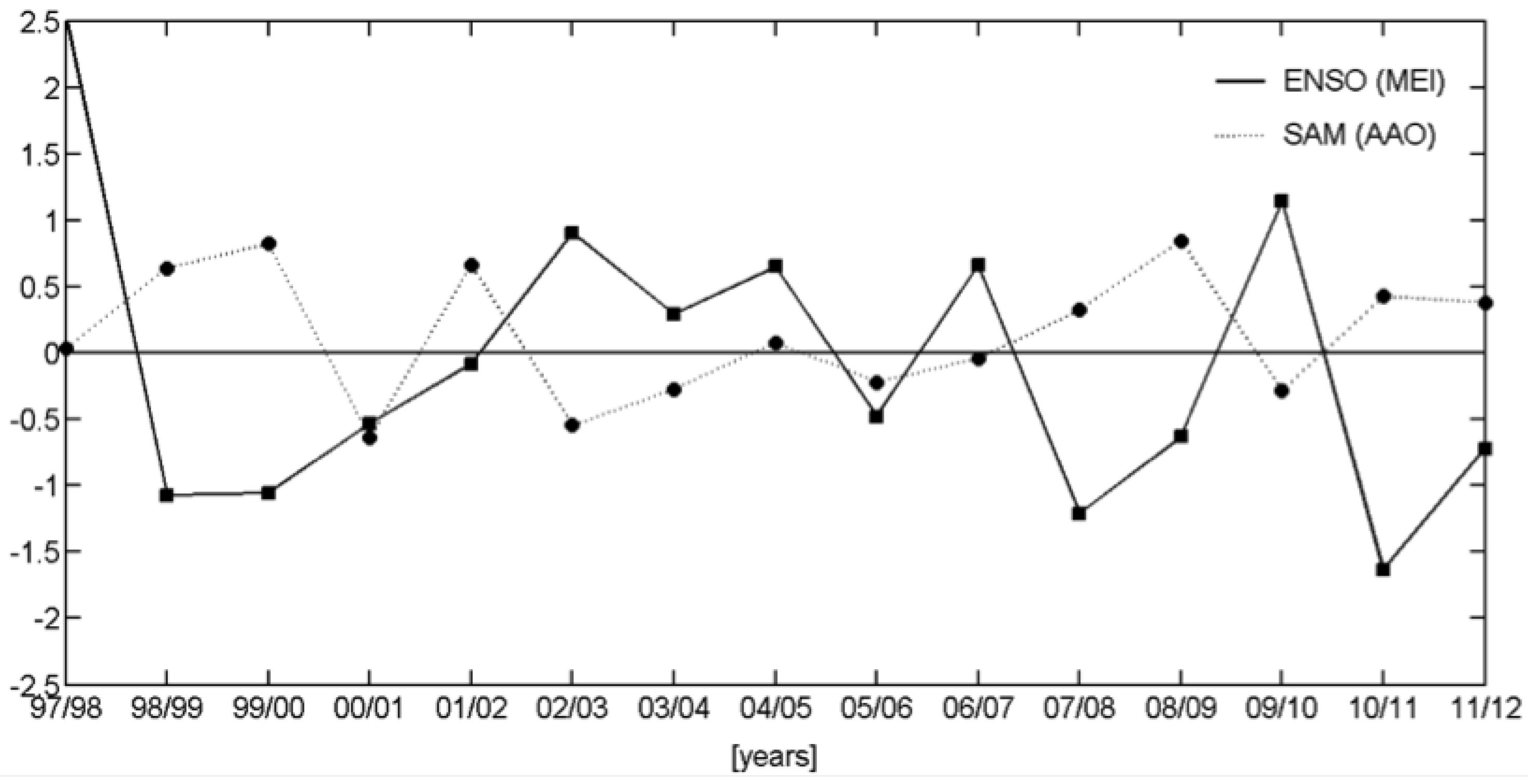
2.4. Climate Indices

To investigate if the Dia-Chla phenology in the Southern Ocean is influenced by ENSO and SAM climate oscillations, we used two indices: the Multivariate El Niño Southern Oscillation index (MEI) and the Antarctic Oscillation (AAO) index. The MEI, available at http://www.esrl.noaa.gov/ psd/enso/mei/#loadings, is based on six variables (cloudiness, sea surface temperature, sea-level pressure, surface air temperature and the zonal and meridional components of the surface wind) over the tropical Pacific from 30 N to 30 S [46]. Positive MEI values can characterize El Niño events while negative values indicate La Niña events. The Antarctic Oscillation (AAO) index, available at http://www.cpc.ncep.noaa.gov/products/precip/CWlink/daily_ao index/ aao/monthly.aao.index.b79.current.ascii.table, is based on the first principal component of monthly mean pressure anomalies at 700 mb for the region south of 30 S [47]. Positive/negative phases of the Southern Annular Mode (SAM) are associated with positive/negative values of AAO, respectively.
Annual ENSO and SAM indices were calculated by averaging their respective indices from September of the previous year to April of the following year, the same period used to estimate the phenological indices. During the 1997–2012 period there were six El Niño years (1997/1998, 2002/2003, 2003/2004, 2004/2005, 2006/2007, 2009/2010), eight La Niña years (1998/1999, 1999/2000, 2000/2001, 2005/2006, 2007/2008, 2008/2009, 2010/2011, 2011/2012), seven years of a positive phase of SAM (1998/1999, 1999/2000, 2001/2002, 2007/2008, 2008/2009, 2010/2011, 2011/2012) and four of a negative phase (2000/2001, 2002/2003, 2003/2004, 2009/2010) (Figure 1 and Table 1).

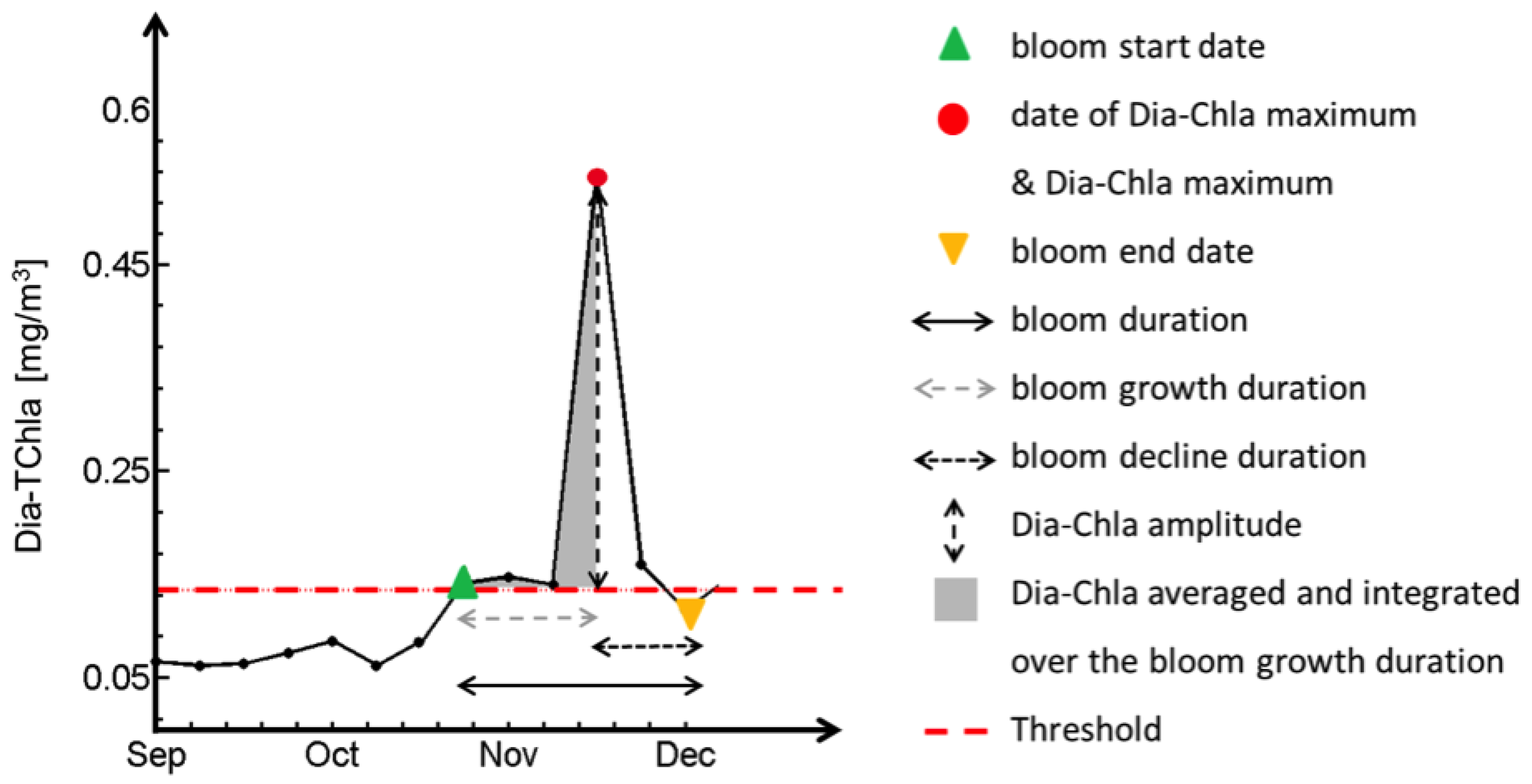
2.5. Phenological Indices

We assessed the diatom phenology using a threshold method initially developed based on the total chlorophyll-a concentration [48]. We note that there are different methods to estimate the bloom phenology. Here we use a robust and widely applied method to investigate phytoplankton phenology from ocean colour data [5,9,48,49,50,51].
Phytoplankton blooms start (defining the bloom start date - BSD) when the Chla value exceeds a value of 5% above the median [48] and remains above this threshold for at least two consecutive weeks [9] (Table 2 and Figure 2). To isolate primary blooms from secondary blooms, we first identified the maximum Dia-Chla of the time series and then looked backwards in time to find the bloom start date [51]. The bloom end date (BED) was determined as the first week when Dia-Chla level fell below the threshold. The period between bloom start date and end date defines the total bloom duration (BD). Within this period the Dia-Chla reaches a maximum (CM) at the date of Dia-Chla maximum (CMD). The sub-periods before and after the maximum determine the bloom growth duration (BGD) and bloom decline duration (BDD), respectively. During the growth duration, the average (CAV) and integrated Dia-Chla values (CI) are calculated. In addition, the amplitude of the bloom (CA) is determined as the difference between maximum and threshold Dia-Chla value.
Using these indices, we analyzed the phenology of the entire time series (1997 to 2012), from September to April of the following year (e.g., September 2002–April 2003). Before computing the phenological indices, the time series were linearly interpolated in time to fill gaps less than 3 weeks in length [49]. After the temporal interpolation, if there were remaining gaps of more than two weeks between the date of Dia-Chla maximum and the estimated bloom start or bloom end date, these phenological indices were not calculated to avoid erroneous detection of the bloom timing. This led to slightly different data coverage of the phenological indices. The best data coverage is achieved for date of Dia-Chla maximum, Dia-Chla maximum and amplitude of the bloom.

2.6. Statistical Analysis

The mean spatial patterns were obtained by averaging the 15 years of phenological indices. To examine the interannual variability of the diatom phenology, we estimated the trends, correlations with ENSO and SAM indices and composite maps of the anomaly of the phenological indices. The analyses were performed using the standardized anomaly data. Standardized anomalies (dimensionless and hereafter termed as anomalies) were produced by subtracting the average (15-yr) from the annual phenology data (e.g., 2002–2003) and dividing by the standard deviation (15-yr), pixel by pixel. Trends were investigated with non-parametric Kendall’s tau test with Sen’s method at the 95% confidence level for each grid cell (only when 100% of data were available). End-point bias was not accounted for. The correlation between the climate indices and anomalies of the phenological indices was determined using Spearman correlation. Partial correlations were used to study the influence of both oscillations separately, for example, by considering the relationship between SAM and Dia-Chla maximum after removal of the effect of ENSO [21], since the correlation between the annual ENSO and SAM indices is −0.58 (p-value = 0.03). Composite maps of the anomalies of the phenological indices were computed by averaging the anomalies from the different phases (positive/negative) of ENSO and SAM. Using composite maps we investigated the dominant patterns of the anomalies associated with the different phases and oscillations [52]. Unfortunately, because of the short length of our time series it was not possible to distinguish between amplified (e.g., El Niño coincided with negative phase of SAM) and non-amplified years (Table 1).

3. Results and Discussion
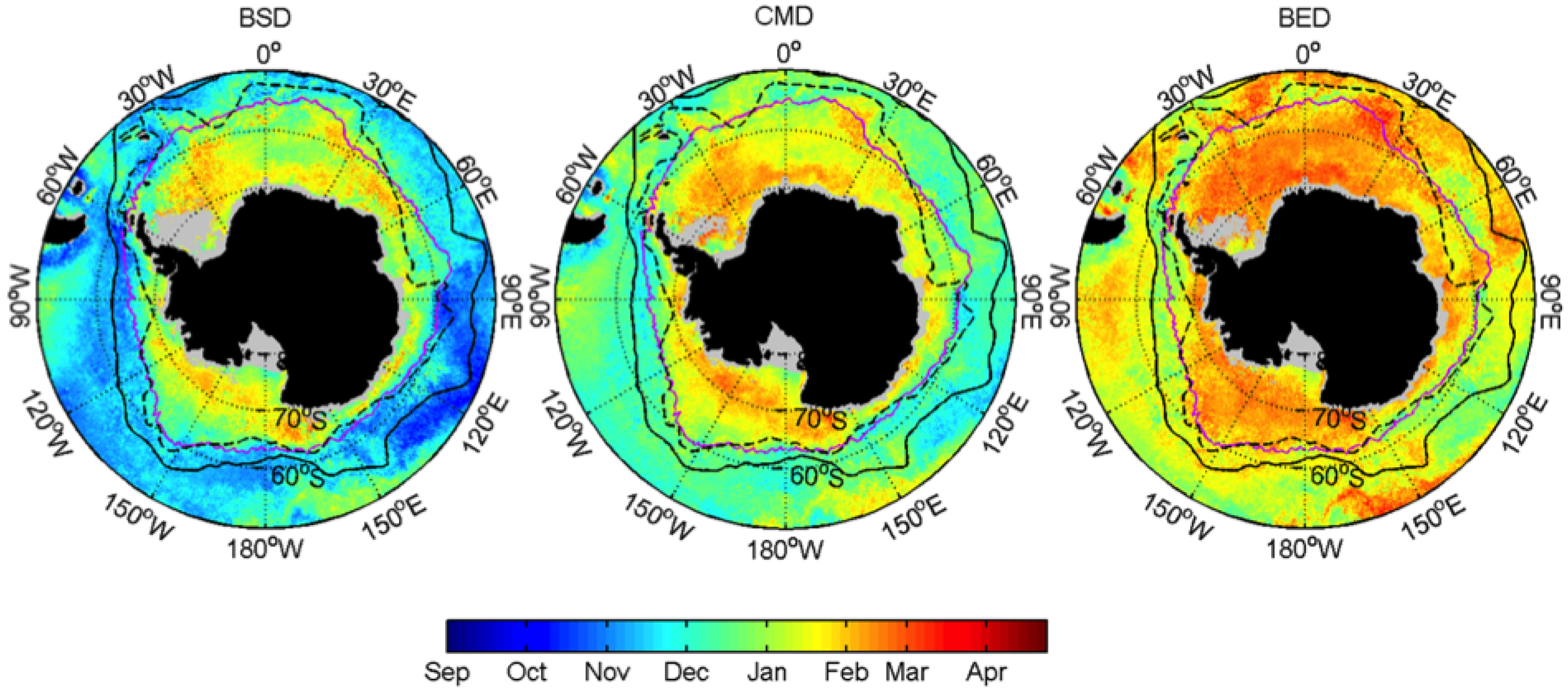
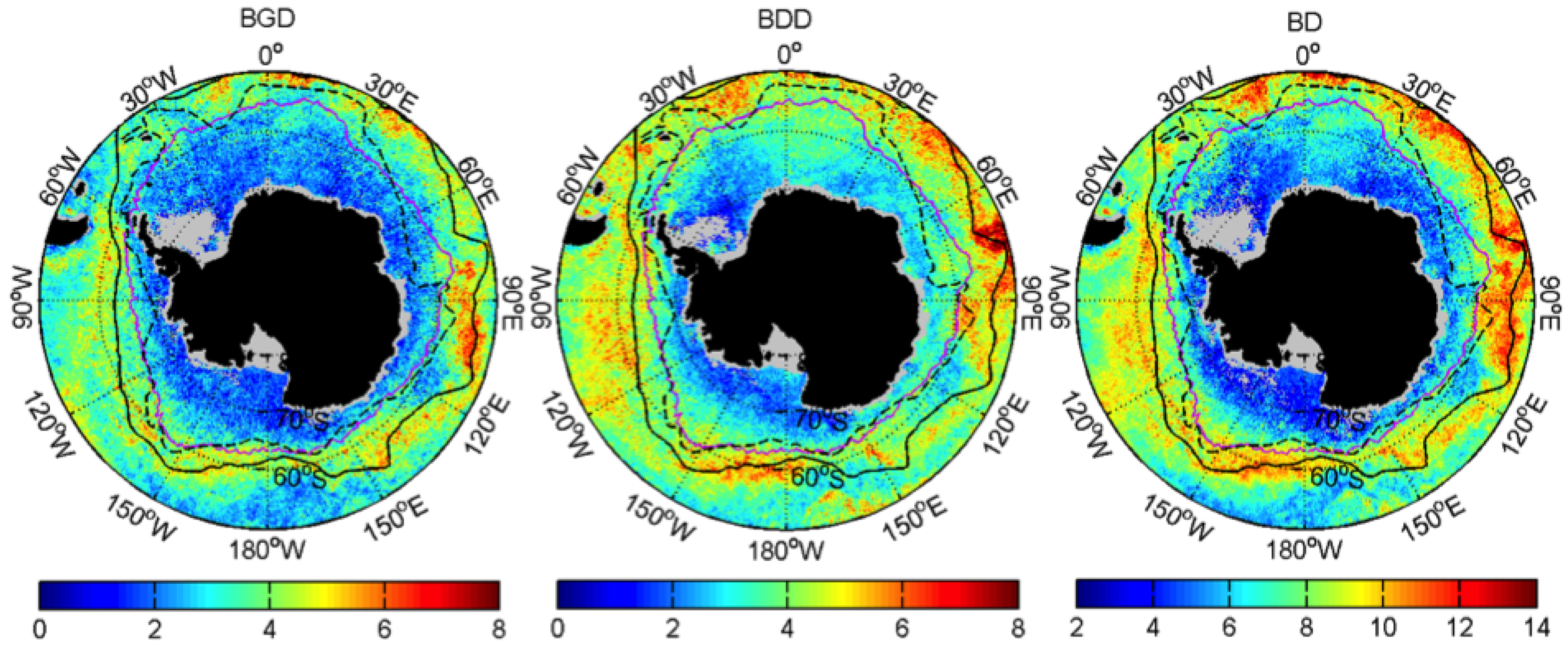
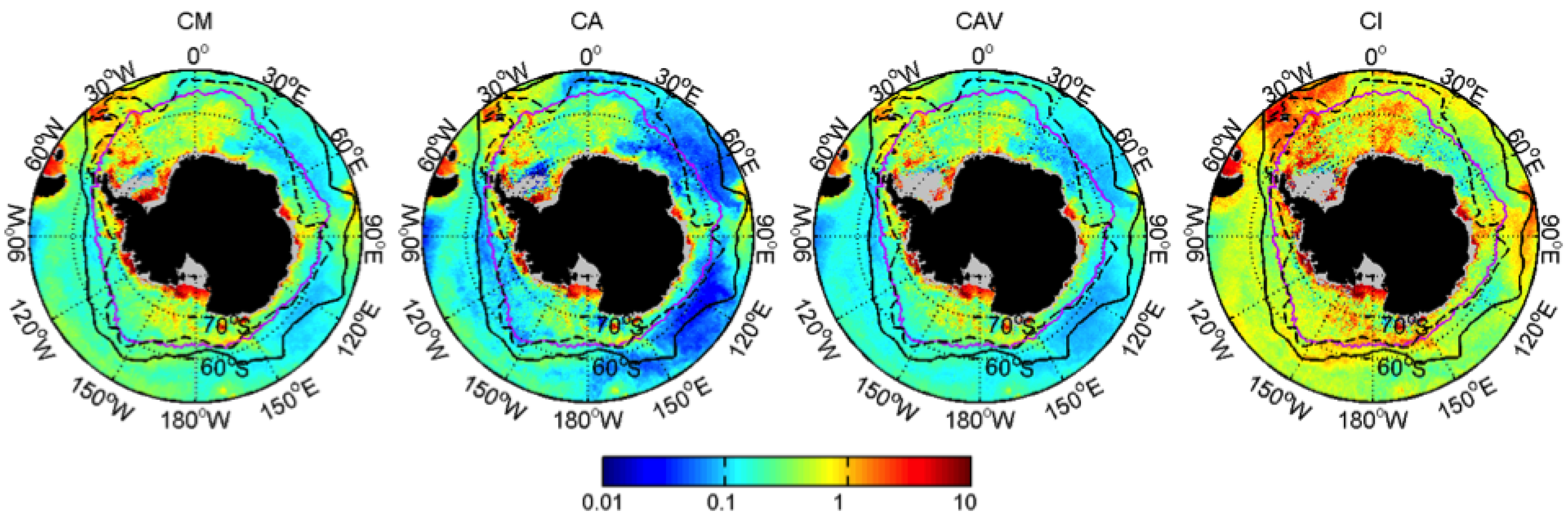
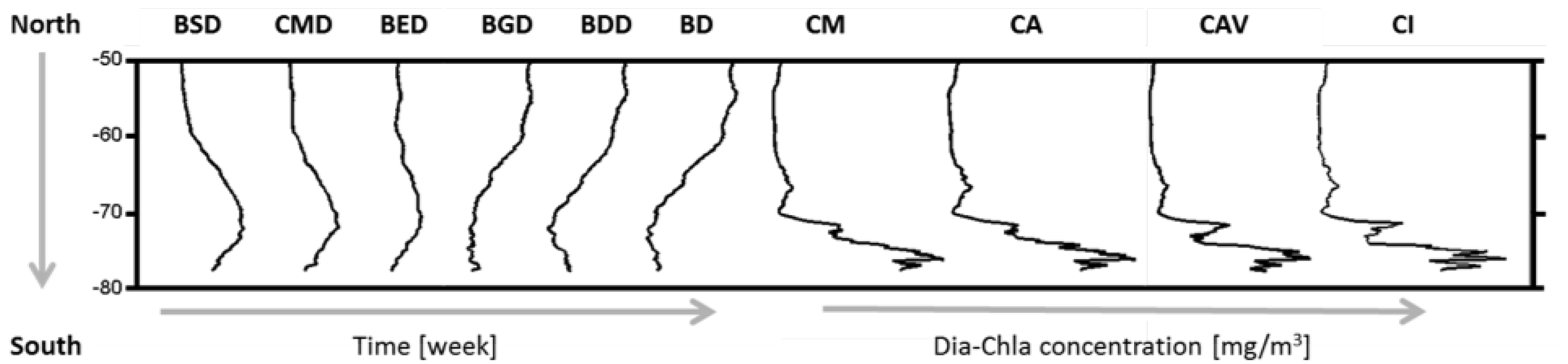
3.1. Mean Patterns

The spatial patterns of the diatom phenological indices averaged over the 15-year period are presented in Figure 3 to Figure 5, together with the corresponding latitudinal variation in Figure 6. Overall, the spatial patterns are associated to the location of the contour of the SACCF and of the maximum sea ice extent. This association is particularly clear for the bloom start date, maximum date, growth duration and total duration of the diatom blooms. The diatom blooms start and reach their maximum earlier north of the SACCF–outside the seasonal ice zone (Figure 3). The spatial pattern of the bloom start date is consistent with [9] and mainly follows the increase in light availability [5,9]. On the other hand, the end of the bloom is more likely related to the exhaustion of nutrients [25,26,28]. In the South Georgia region the exhaustion of silicate is thought to be a limiting factor for the end of the spring diatom bloom [11]. Grazing pressure is thought to control the diatom species composition and biomass, rather than the end of the diatom bloom [28]. In the seasonal ice zone, the start of the bloom is driven by light as well as water column stability; as the sea ice retreats, the melting of ice increases the stratification of the water column which favors to maintain the phytoplankton in the euphotic zone [12]. The end of the bloom occurs when the mixed layer deepens due to wind forcing, which dilutes the phytoplankton in the water column [12] and can bring them to lower light levels.
Particularly notable is the early start of the diatom blooms in the waters surrounding Antarctica in December (light green), caused by the opening of areas free of ice around the continent. Arrigo et al. [53] showed that in the Amundsen polynya small areas free of ice occur throughout the year and that their size increases with three factors: advection of sea ice offshore, increase in temperature and melting of ice. These factors, combined with an increase in solar radiation and water column stability, as shown by [12], are linked to the earlier bloom start date in these waters surrounding Antarctica as compared to other regions of the seasonal ice zone.
The duration of the diatom blooms is shorter south of the SACCF, in the seasonal ice zone, and vice versa (Figure 4). Outside this region it forms a belt of higher values (longer duration) around the Polar Front (PF), particularly between 30 W and 120 E. Previous phenology studies (e.g., [3,4,5,9]) based on total Chla data, which includes all PFTs, reported durations of phytoplankton blooms, which were longer than the durations of the diatom blooms observed in the present study. Specifically, the average duration of the blooms for the regions 50 S–60 S and 60 S–70 S was 8.3 and 6.5 weeks for the diatom blooms, while total chla blooms were shown to range between 14 and 11 weeks [5], respectively.
The duration of the bloom in the seasonal ice zone results from a combination of factors influencing the growth and decline phases of the bloom, mainly light and stability of the water column, while nutrients are less important [12]. The belt of ’longer lasting’ blooms outside the seasonal ice zone is likely linked to a complex inter-play of different forcings: longer light periods and deeper mixed layers [54] that enhance the supply of nutrients at surface as well as reduce the grazing pressure by zooplankton [55]. The mixed layer depth is deeper in the vicinity the fronts; around 100 m in the summer and up to 400 m in the winter [54].
The deepening of the mixed layer in the winter together with diapycnal diffusion replenishes the surface with nutrients from subsurface waters, including iron [56]. It is known that iron is a limiting nutrient in the surface waters of the Southern Ocean controlling phytoplankton growth, particularly in the open ocean. This micronutrient is rapidly depleted by spring blooms. In late spring and summer, phytoplankton relies on the pelagic recycling until the following deepening of the mixed layer in autumn [56]. Open ocean diatoms have the ability to reduce their requirement of iron [23] which can help to sustain their blooms for longer periods. Other important factors controlling the duration of the bloom are the increasing of grazing pressure and algal viruses [28,55].
The relationship of the biomass indices with the fronts is not as evident as for the other indices (Figure 5). The spatial distribution shows that more intense diatom blooms (higher biomass) occur in coastal regions, in the seasonal ice zone and in the Atlantic sector of the Southern Ocean. Diatom blooms around Antarctica can be considered as more efficient blooms, with short duration and high biomass. Sokolov and Rintoul [57] have shown that at a broader scale the distribution of Chla is mainly controlled by the upwelling of nutrients via Ekman transport while the upwelling associated with bathymetric features is responsible for the magnitude and duration of the blooms. In regions where the Antarctic Circumpolar Front (ACC) interacts with the topography, the nutrient supply is enhanced [57] leading to higher Chla and consequently, higher amplitude of the blooms. This occurs for example in the Pacific Antarctic Ridge (see Figure 7 in [57]). The enrichment from the coastal and shelf sediments close to islands (e.g., Kerguelen, Crozet and South Georgia Islands) are also important sources of nutrients, especially iron [58,59,60].
The latitudinal variability displays, from north to south, a progressive delay in the start, maximum and end date of the diatom blooms until about 73 S (Figure 6). The opposite is observed for the duration; there is a decrease in the growth, decline and total duration of the diatom blooms from north to south. South of 73 S the trend is reversed except by the growth duration which holds at about the same duration. The biomass indices present similar latitudinal variations, but are rather small until the first peak at ~67 S, followed by two steep peaks at ~72 S and at ~76 S, and then decreasing towards the south.
The computation of the phenological indices reported here may not only be affected by the data drawbacks mentioned in the methods (missing the deep Chla maximum, gaps), but also satellite pixels contaminated by white caps, sea ice or sun glint can potentially affect the results. Ocean colour data in polar oceans are known to have issues related to sea ice, low sun elevation, clouds and polar aerosols [61]. Adjacency effect and sea ice contaminated pixels can lead to overestimation of the satellite Chla and standard SeaWiFS and MODIS flags may not remove all impacted pixels [62,63]. The extent of these issues in the timing of the diatom blooms has not been yet quantified and needs more attention. By using the OC-CCI Chla product in this study, where POLYMER is used for the MERIS atmospheric correction, we believe to work with the best long term dataset available for the Southern Ocean.

3.2. Interannual Variability
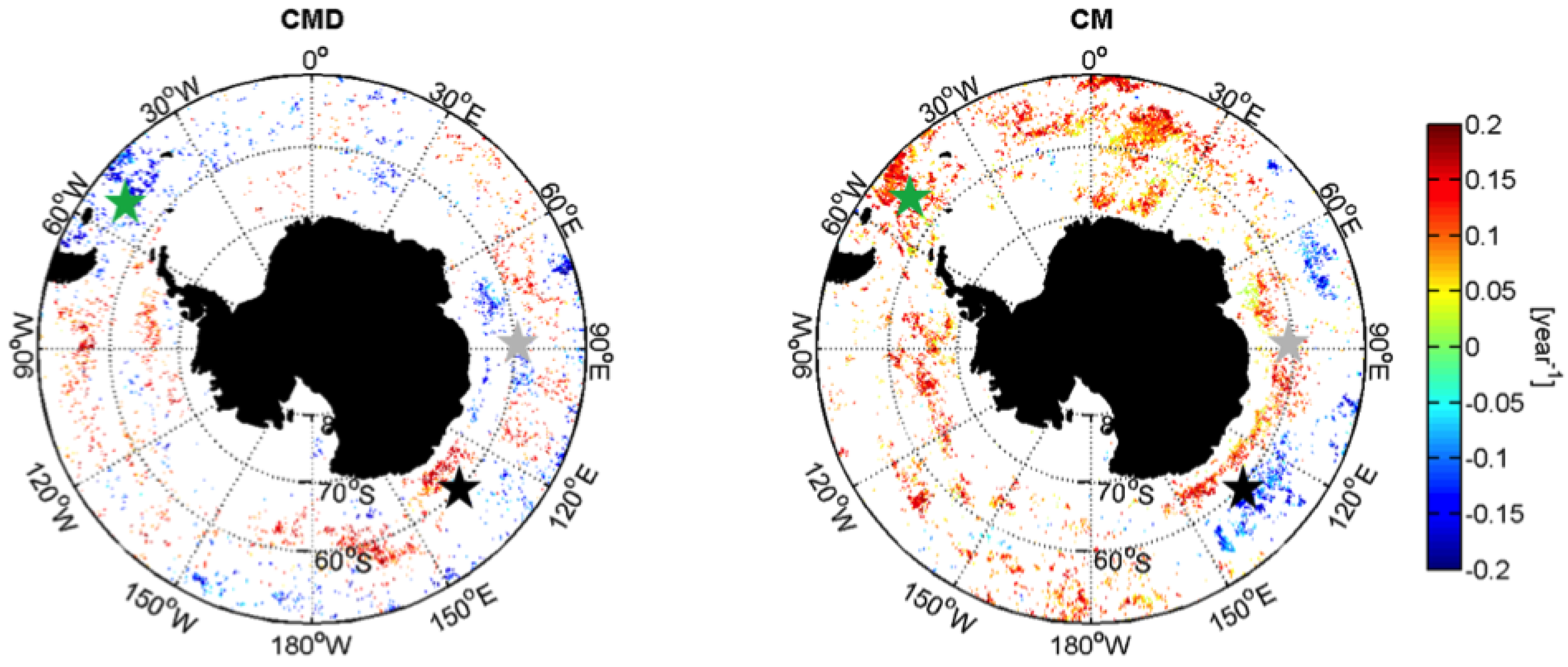
3.2.1. Trends

Because among the phenological indices only the Dia-Chla maximum, Dia-Chla maximum and amplitude indices are gap free, trends could only be determined for those indices. Trends in the Dia-Chla amplitude are very similar to Dia-Chla maximum and not shown.
Coherent patches of significant positive and negative trends were detected for the date of Dia-Chla maximum and Dia-Chla maximum (Figure 7). For example, in the region between the Malvinas and South Georgia Islands (Figure 7, green star) there is a trend towards an earlier maximum of the bloom leading to higher biomass (Dia-Chla maximum). However, the opposite relationship where a later start of the bloom leads to an increase in biomass can also be observed (e.g., in the region south of 60 S and between 120 E and 150 E) (Figure 7, black star). Although we could not estimate trends in the bloom start date and bloom end date, we can expect a similar pattern to the ones detected for date of Dia-Chla maximum since these indices are highly correlated (Figure S1 in the supplement).
These observations combined with recent studies on the trends in sea surface temperature [64] and sea ice cover [65] over the last three decades, suggest a link between these two variables and the diatom phenology. For example, in the region south of 60 S and from 60 E to 120 E (Figure 7, grey star) the earlier date of Dia-Chla maximum and the increased Dia-Chla maximum coincide with the observed increase trend in SST and decrease in sea ice cover (earlier sea ice melt).
Compared to literature, the spatial distribution of trends in Dia-Chla maximum are similar to trends in total Chla from SeaWiFS reported by [66] and [67] for the 1997–2007 and 1997–2010 periods, respectively. Recent decadal trends (1998–2012) in diatom concentration have been investigated by [68] based on model results, where large areas in the Southern Ocean with positive trends have been observed as in this study (e.g., off the Patagonian shelf), but also positive trends between the 60 E and 150 E north of 60 S whereas we observed negative trends. Furthermore, the general increase in Dia-Chla maximum observed here coincide with regions where [68] observed a shallowing of the MLD and an increase in silicate, iron and nitrate.

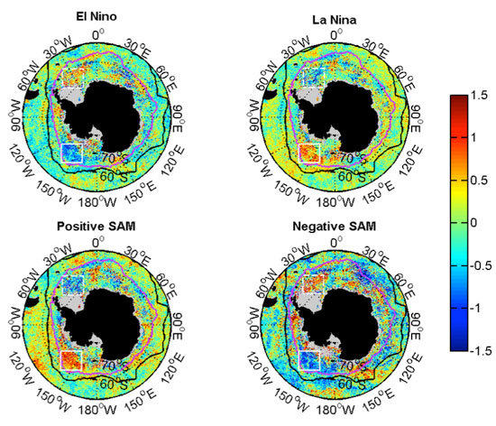
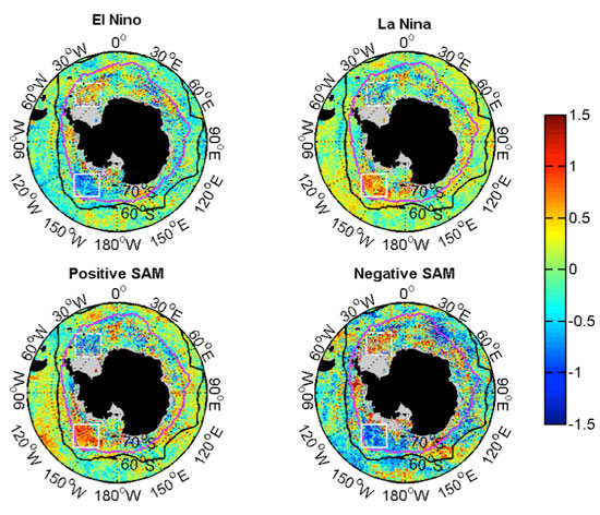
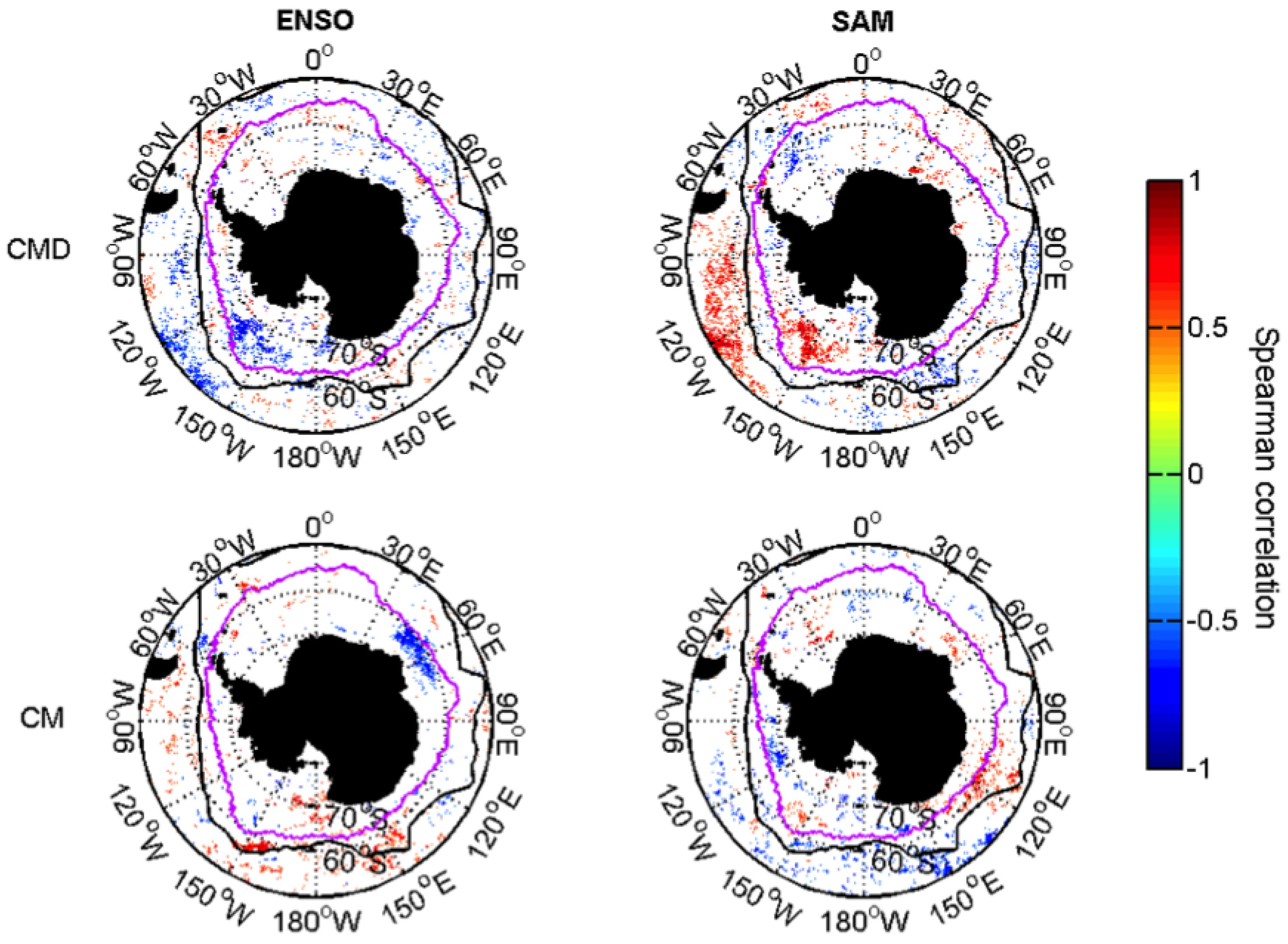
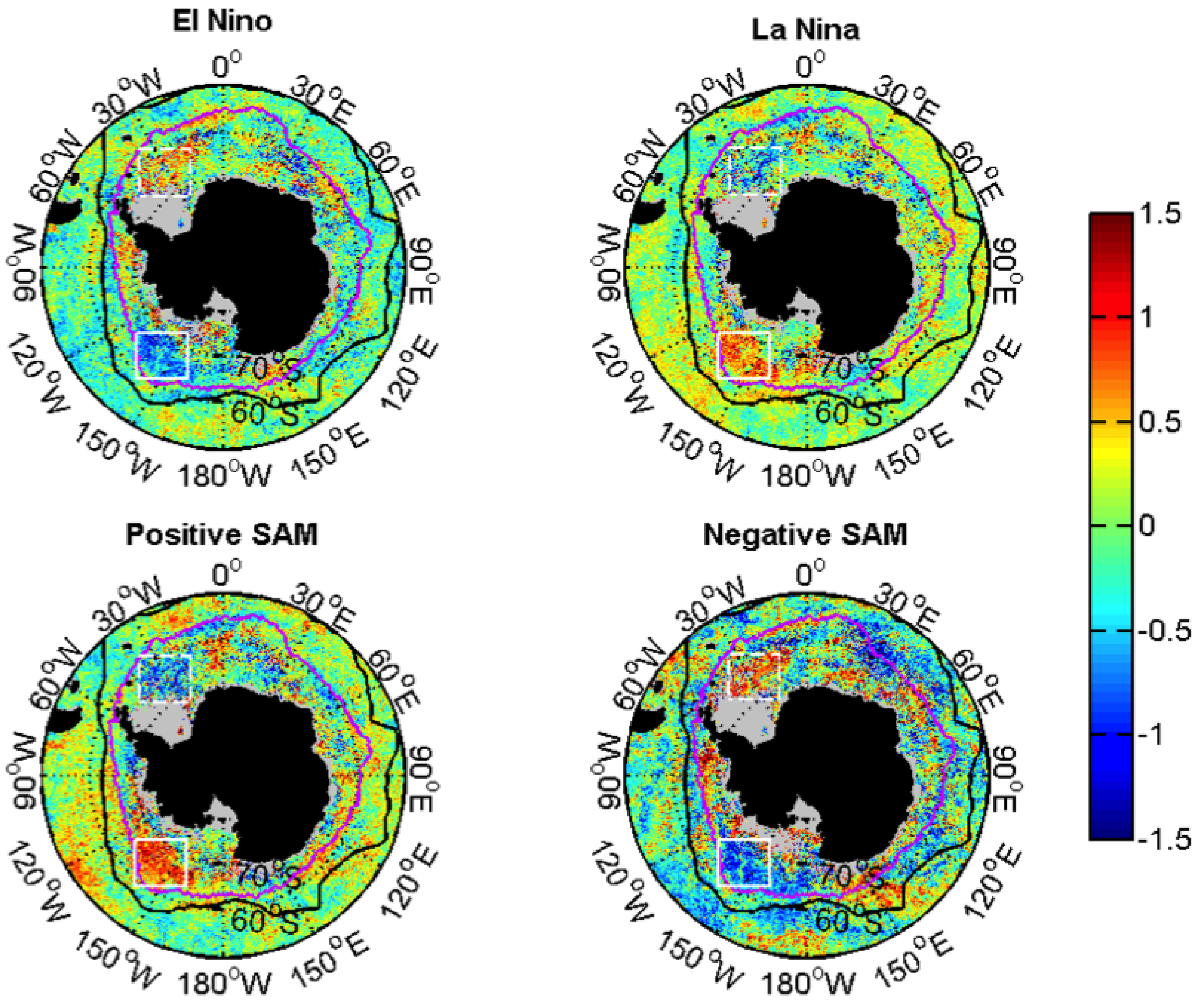
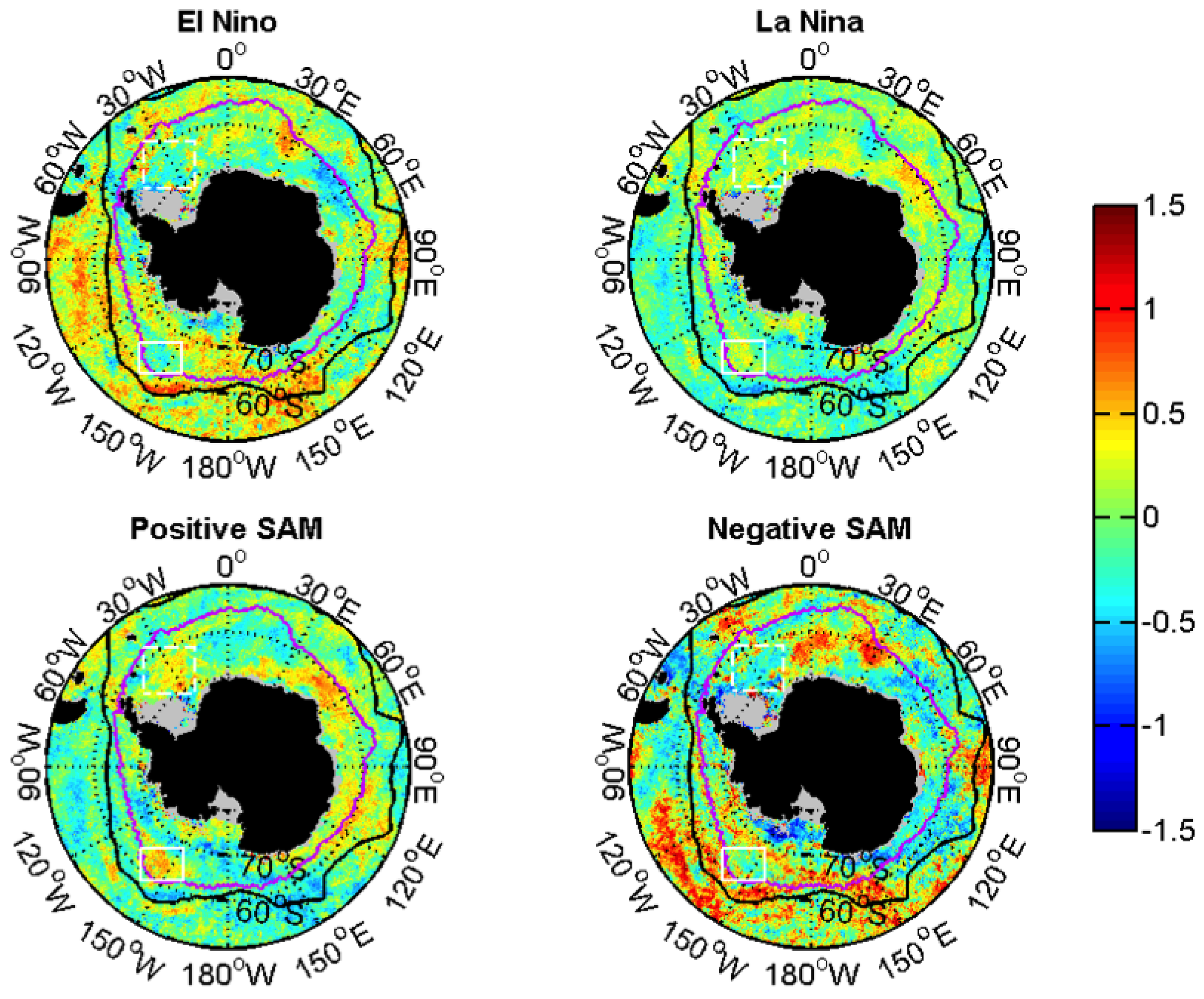
3.2.2. Relationships with ENSO and SAM

To further explore the interannual variability of the diatom phenology, we examined the relationship of the annual phenological indices with ENSO and SAM. The correlation maps are presented in Figure 8 for date of Dia-Chla maximum and Dia-Chla maximum as representative of the date indices and biomass indices, respectively. Significant positive (negative) correlations indicate that the anomalies are in (out of) phase with ENSO and SAM. Consistent areas in the duration indices are less evident for the duration indices.
Several areas show significant correlation between ENSO and SAM and the diatom phenology. The correlation coefficients for ENSO are opposite to that of SAM. For example, the date of Dia-Chla maximum in the sector of the seasonal ice zone between 120 W and 150 W is negatively correlated with ENSO and positively correlated with SAM. Moreover, the patterns in El Niño (La Niña) years and negative (positive) SAM are similar. These results are in line with observations of the sea ice concentration, SST, Chla and wind speed and direction in the Southern Ocean [20,21]. Smith et al. [15] also observed that high Chla biomass offshore the Western Antarctic Peninsula region was associated La Niña and/or positive SAM events. Hence, we can expect the spatial patterns of the anomalies of phenological indices during El Niño (La Niña) years and negative (positive) phase of SAM to resemble each other.
The most remarkable feature in the correlation maps of the date of Dia-Chla maximum can be seen in the Pacific Sector (90 W to 150 W), north of the PF and south of the maximum sea ice extent. This is consistent with patterns observed by [52,69] for earlier periods, 1982–1998 and 1980–1999 and using satellite and model data, respectively. For the same region, Kwok and Comiso [52] observed an increase in SST and a decline in sea ice concentration associated with El Niño. Lefebvre et al. [69] showed that the winter sea ice concentration decreases in negative SAM events. As a result, an earlier start, maximum and end of the bloom can be expected in El Niño or negative SAM events.
The Dia-Chla maximum displays less significant correlations, but the general pattern of Dia-Chla maximum is consistent with the correlations of satellite Chla and SAM presented by [22] for an earlier period (1997–2004). The observed lower Dia-Chla maximum at 60 E during El Niño (negative correlation) can be linked to lower SST in El Niño years, as shown by [52] (see Figure 6 in [52]). In contrast, the general increase in diatom concentration between 50 S and 70 S during positive SAM event showed by [70] was not observed in our results. The authors used a coupled ecosystem-general circulation model and lagged correlations (4 months) to investigate the relationship and these might be the cause for disagreement between the results, as well as the different periods analyzed in their study (1948–2010) and in the present study (1997–2012).
Because SAM and ENSO are not linearly independent at interannual time scales during the austral summer season [21,71], we expect that some of the variability we observed related to SAM may be influenced by ENSO, or vice versa. This was in part confirmed by the partial correlations (Figure S2 in the supplement), but the differences between the correlations and partial correlations are in general small. Higher differences were observed between the date of Dia-Chla maximum and MEI. The correlations between the date of Dia-Chla maximum and SAM, and Dia-Chla maximum and MEI or SAM did not change. One possible reason for not observing differences is that the short time series used here might not allow to distinguish the influence of the respective oscillations, reinforcing the need for continuous and longer ocean colour records.
The composite maps of the anomalies of bloom start date, Dia-Chla maximum and bloom duration are shown in Figure 9 and Figure 10 and Figure S3 in the supplement, respectively, and provide insight into the magnitude of the anomalies during the ENSO and SAM events. In the seasonal ice zone there are two regions with inverse patterns and high anomalies of bloom start date: the Weddell Sea region (white dashed box) and the sector between 120 W and 180 W (white box), north of 70 S. In the Weddell Sea, El Niño/negative SAM years are characterized by later start, shorter duration and slightly higher diatom biomass, which are likely a response of more extensive ice cover in these years [52,69]. In the sector between 120 W and 180 W the pattern presents opposite sign.

4. Conclusions

Over the last decade, the phenology of phytoplankton blooms in the Southern Ocean has been examined using satellite-derived estimates of Chla [3,9,10]. However, by looking at the total Chla provided by satellite no information about the phytoplankton community composition (and changes in) is provided [72]. In this study we were able to look specifically at the diatom biomass by using a satellite-derived diatom concentration. We investigated the mean spatial and temporal patterns of diatom phenology and their interannual variability. We find a clear correspondence between ENSO and SAM and the phenology of diatoms, as revealed by the correlation and the anomaly composite maps. The influence of the climate oscillations varies depending on the region. It is also evident that ENSO and SAM have opposite effects in the diatom phenology. These results emphasize the influence of climate oscillations on the diatom phenology in the Southern Ocean.
A next step would be to investigate in more detail the relationship between climate oscillations, environmental variables and diatom phenology. Such investigation is not straight forward and requires a comprehensive dataset of, at least, weekly temporal resolved data including not only information on SST and PAR, as usual used in phytoplankton phenology studies since these variables are freely available from remote sensing, but also information on e.g., water column mixing, sea ice concentration, dissolved iron and silicate and grazing pressure. Combining remote sensing and model data can help to explain the missing link between climate oscillations, environmental anomalies and diatom bloom phenology.
Last, the knowledge of other phytoplankton types forming blooms in the Southern Ocean, mainly haptophytes, is essential to understand phytoplankton community shift and the factors controlling it. E. huxleyi are known to occur along the ’Great Calcite Belt’ and dense blooms are often observed at the shelf break and off the Patagonian shelf after the spring bloom of diatoms. Moreover, while it is generally accepted that diatoms dominate the spring bloom in the Southern Ocean [26] this might not be true everywhere as the spring bloom of P. antarctica in the Ross Sea [73].

Supplementary Files

Supplementary File 1

Acknowledgments

We would like to acknowledge the Ocean Colour CCI project for the production and distribution of the chlorophyll data. This work was partially supported by the Alfred-Wegener-Institute, the Total Foundation Project “Phytoscope” and the ESA-SEOM SY-4SCI SYNERGY project “SynSenPFT”.

Author Contributions

Mariana Soppa led the study, performed data analysis and wrote the manuscript. Christoph Völker and Astrid Bracher were involved in discussions and assisted in writing the manuscript.

Conflicts of Interest

The authors declare no conflict of interest.

References

  1. Kahru, M.; Brotas, V.; Manzano-sarabia, M.; Mitchell, B. Are phytoplankton blooms occurring earlier in the Arctic? Glob. Change Biol. 2011, 17, 1733–1739. [Google Scholar] [CrossRef]
  2. Ardyna, M.; Babin, M.; Gosselin, M.; Devred, E.; Rainville, L.; Tremblay, J.É. Recent Arctic Ocean sea ice loss triggers novel fall phytoplankton blooms. Geophys. Res. Lett. 2014, 41, 6207–6212. [Google Scholar] [CrossRef]
  3. Carranza, M.M.; Gille, S.T. Southern Ocean wind-driven entrainment enhances satellite chlorophyll-a through the summer. J. Geophys. Res.: Oceans 2015, 120, 304–323. [Google Scholar] [CrossRef]
  4. Cole, H.S.; Henson, S.; Martin, A.P.; Yool, A. Basin-wide mechanisms for spring bloom initiation: How typical is the North Atlantic? ICES J. Mar. Sci.: J. Conseil 2015, 72, 2029–2040. [Google Scholar] [CrossRef]
  5. Racault, M.F.; Le Quéré, C.; Buitenhuis, E.; Sathyendranath, S.; Platt, T. Phytoplankton phenology in the global ocean. Ecol. Indic. 2012, 14, 152–163. [Google Scholar] [CrossRef]
  6. Edwards, M.; Richardson, A.J. Impact of climate change on marine pelagic phenology and trophic mismatch. Nature 2004, 430, 881–884. [Google Scholar] [CrossRef] [PubMed]
  7. Platt, T.; Fuentes-Yaco, C.; Frank, K.T. Marine ecology: Spring algal bloom and larval fish survival. Nature 2003, 423, 398–399. [Google Scholar] [CrossRef] [PubMed]
  8. Koeller, P.; Fuentes-Yaco, C.; Platt, T.; Sathyendranath, S.; Richards, A.; Ouellet, P.; Orr, D.; Skúladóttir, U.; Wieland, K.; Savard, L.; et al. Basin-scale coherence in phenology of shrimps and phytoplankton in the North Atlantic Ocean. Science 2009, 324, 791–793. [Google Scholar] [CrossRef] [PubMed]
  9. Thomalla, S.; Fauchereau, N.; Swart, S.; Monteiro, P. Regional scale characteristics of the seasonal cycle of chlorophyll in the Southern Ocean. Biogeosciences 2011, 8, 2849–2866. [Google Scholar] [CrossRef]
  10. Sallée, J.B.; Llort, J.; Tagliabue, A.; Lévy, M. Characterization of distinct bloom phenology regimes in the Southern Ocean. ICES J. Mar. Sci.: J. Conseil 2015, 72, 1985–1998. [Google Scholar] [CrossRef]
  11. Borrione, I.; Schlitzer, R. Distribution and recurrence of phytoplankton blooms around South Georgia, Southern Ocean. Biogeosciences 2013, 10, 217–231. [Google Scholar] [CrossRef] [Green Version]
  12. Taylor, M.H.; Losch, M.; Bracher, A. On the drivers of phytoplankton blooms in the Antarctic marginal ice zone: A modeling approach. J. Geophys. Res.: Oceans 2013, 118, 63–75. [Google Scholar] [CrossRef] [Green Version]
  13. Arrigo, K.R.; van Dijken, G.L. Annual cycles of sea ice and phytoplankton in Cape Bathurst polynya, southeastern Beaufort Sea, Canadian Arctic. Geophys. Res. Lett. 2004. [Google Scholar] [CrossRef]
  14. Montes-Hugo, M.; Vernet, M.; Martinson, D.; Smith, R.; Iannuzzi, R. Variability on phytoplankton size structure in the western Antarctic Peninsula (1997–2006). Deep Sea Res. Part II: Top. Stud. Oceanogr. 2008, 55, 2106–2117. [Google Scholar] [CrossRef]
  15. Smith, R.C.; Martinson, D.G.; Stammerjohn, S.E.; Iannuzzi, R.A.; Ireson, K. Bellingshausen and western Antarctic Peninsula region: Pigment biomass and sea-ice spatial/temporal distributions and interannual variabilty. Deep Sea Res. Part II: Top. Stud. Oceanogr. 2008, 55, 1949–1963. [Google Scholar] [CrossRef]
  16. Alvain, S.; Le Quéré, C.; Bopp, L.; Racault, M.F.; Beaugrand, G.; Dessailly, D.; Buitenhuis, E.T. Rapid climatic driven shifts of diatoms at high latitudes. Remote Sens. Environ. 2013, 132, 195–201. [Google Scholar] [CrossRef]
  17. McPhaden, M.J.; Zebiak, S.E.; Glantz, M.H. ENSO as an integrating concept in earth science. Science 2006, 314, 1740–1745. [Google Scholar] [CrossRef] [PubMed]
  18. Thompson, D.W.; Wallace, J.M. Annular modes in the extratropical circulation. Part I: Month-to-month variability*. J. Clim. 2000, 13, 1000–1016. [Google Scholar] [CrossRef]
  19. Penland, C.; Sun, D.Z.; Capotondi, A.; Vimont, D.J. A brief introduction to El Nino and La Nina. In Climate Dynamics: Why Does Climate Vary? Elsevier: Amsterdam, The Netherlands, 2010; pp. 53–64. [Google Scholar]
  20. Lovenduski, N.S. Impact of the Southern Annular Mode on Southern Ocean Circulation and Biogeochemistry; University of California: Los Angeles, CA, USA, 2007. [Google Scholar]
  21. Pohl, B.; Fauchereau, N.; Reason, C.; Rouault, M. Relationships between the Antarctic Oscillation, the Madden-Julian Oscillation, and ENSO, and consequences for rainfall analysis. J. Clim. 2010, 23, 238–254. [Google Scholar] [CrossRef]
  22. Lovenduski, N.S.; Gruber, N. Impact of the Southern Annular Mode on Southern Ocean circulation and biology. Geophys. Res. Lett. 2005. [Google Scholar] [CrossRef]
  23. Armbrust, E.V. The life of diatoms in the world’s oceans. Nature 2009, 459, 185–192. [Google Scholar] [CrossRef] [PubMed]
  24. Kooistra, W.; Gersonde, R.; Medlin, L.K.; Mann, D.G. The origin and evolution of the diatoms: Their adaptation to a planktonic existence. In Evolution of Primary Producers in the Sea; Elsevier: Amsterdam, The Netherlands, 2007; pp. 207–249. [Google Scholar]
  25. Smetacek, V. Diatoms and the ocean carbon cycle. Protist 1999, 150, 25–32. [Google Scholar] [CrossRef]
  26. Smetacek, V. Role of sinking in diatom life-history cycles: Ecological, evolutionary and geological significance. Mar. Biol. 1985, 84, 239–251. [Google Scholar] [CrossRef]
  27. Raven, J.; Waite, A. The evolution of silicification in diatoms: Inescapable sinking and sinking as escape? New Phytol. 2004, 162, 45–61. [Google Scholar] [CrossRef]
  28. Smetacek, V.; Assmy, P.; Henjes, J. The role of grazing in structuring Southern Ocean pelagic ecosystems and biogeochemical cycles. Antarct. Sci. 2004, 16, 541–558. [Google Scholar] [CrossRef]
  29. Assmy, P.; Smetacek, V.; Montresor, M.; Klaas, C.; Henjes, J.; Strass, V.H.; Arrieta, J.M.; Bathmann, U.; Berg, G.M.; Breitbarth, E.; et al. Thick-shelled, grazer-protected diatoms decouple ocean carbon and silicon cycles in the iron-limited Antarctic Circumpolar Current. Proc. Natl. Acad. Sci. USA 2013, 110, 20633–20638. [Google Scholar] [CrossRef] [PubMed] [Green Version]
  30. Rousseaux, C.S.; Gregg, W.W. Interannual variation in phytoplankton primary production at a global scale. Remote Sens. 2013, 6, 1–19. [Google Scholar] [CrossRef]
  31. Tréguer, P.J.; De La Rocha, C.L. The world ocean silica cycle. Annu. Rev. Mar. Sci. 2013, 5, 477–501. [Google Scholar] [CrossRef] [PubMed]
  32. Tréguer, P.J. The southern ocean silica cycle. Comptes Rendus Geosci. 2014, 346, 279–286. [Google Scholar] [CrossRef]
  33. Sathyendranath, S.; Krasemann, H. Climate Assessment Report: Ocean Colour Climate Change Initiative (OC-CCI) – Phase One. Technical Report, ESA OC-CCI. 2014. Available online: http://www.esa-oceancolour-cci.org/?q=documents (accessed on 9 May 2016).
  34. Steinmetz, F.; Deschamps, P.Y.; Ramon, D. Atmospheric correction in presence of sun glint: Application to MERIS. Opt. Express 2011, 19, 9783–9800. [Google Scholar] [CrossRef] [PubMed]
  35. Wang, M.; Gordon, H.R. A simple, moderately accurate, atmospheric correction algorithm for SeaWiFS. Remote Sens. Environ. 1994, 50, 231–239. [Google Scholar] [CrossRef]
  36. Krasemann, H.; Belo-Couto, A.; Brando, V.; Brewin, R.J.; Brockmann, C.; Brotas, V.; Doerffer, R.; Feng, H.; Frouin, R.; Gould, R.; et al. Product Validation and Inter–Comparison Report; Technical Report 1, Ocean Colour Climate Change Initiative; Helmholtz-Zentrum Geesthacht: Geesthacht, Germany, 2014. [Google Scholar]
  37. Soppa, M.A.; Hirata, T.; Silva, B.; Dinter, T.; Peeken, I.; Wiegmann, S.; Bracher, A. Global Retrieval of Diatom Abundance Based on Phytoplankton Pigments and Satellite Data. Remote Sens. 2014, 6, 10089–10106. [Google Scholar] [CrossRef] [Green Version]
  38. Hirata, T.; Hardman-Mountford, N.; Brewin, R.; Aiken, J.; Barlow, R.; Suzuki, K.; Isada, T.; Howell, E.; Hashioka, T.; Noguchi-Aita, M.; et al. Synoptic relationships between surface Chlorophyll-a and diagnostic pigments specific to phytoplankton functional types. Biogeosciences 2011, 8, 311–327. [Google Scholar] [CrossRef]
  39. Holm-Hansen, O.; Kahru, M.; Hewes, C.D. Deep chlorophyll a maxima (DCMs) in pelagic Antarctic waters. II. Relation to bathymetric features and dissolved iron concentrations. Mar. Ecol. Progr. Ser. 2005, 297, 71–81. [Google Scholar] [CrossRef]
  40. Fennel, K.; Boss, E. Subsurface maxima of phytoplankton and chlorophyll: Steady-state solutions from a simple model. Limnol. Oceanogr. 2003, 48, 1521–1534. [Google Scholar] [CrossRef]
  41. Parslow, J.S.; Boyd, P.W.; Rintoul, S.R.; Griffiths, F.B. A persistent subsurface chlorophyll maximum in the Interpolar Frontal Zone south of Australia: Seasonal progression and implications for phytoplankton-light-nutrient interactions. J. Geophys. Res.: Oceans 2001, 106, 31543–31557. [Google Scholar] [CrossRef]
  42. Racault, M.F.; Sathyendranath, S.; Platt, T. Impact of missing data on the estimation of ecological indicators from satellite ocean-colour time-series. Remote Sens. Environ. 2014, 152, 15–28. [Google Scholar] [CrossRef]
  43. Sallée, J.; Speer, K.; Morrow, R. Southern Ocean fronts and their variability to climate modes. J. Clim. 2008, 21, 3020–3039. [Google Scholar] [CrossRef]
  44. Orsi, A.H.; Whitworth, T.; Nowlin, W.D. On the meridional extent and fronts of the Antarctic Circumpolar Current. Deep Sea Res. Part I: Oceanogr. Res. Pap. 1995, 42, 641–673. [Google Scholar] [CrossRef]
  45. Fetterer, F.; Knowles, K.; Meier, W.; Savoie, M. Sea Ice Index. Boulder, CO: National Snow and Ice Data Center. Digit. Media 2002, 6. Available online: ftp://sidads.colorado.edu/DATASETS/NOAA/G02135/shapefiles/ (accessed on 13 May 2016). [Google Scholar]
  46. Wolter, K.; Timlin, M.S. Monitoring ENSO in COADS with a seasonally adjusted principal component index. In Proceedings of the 17th Climate Diagnostics Workshop, Norman, OK, USA, 18–23 October1993; pp. 52–57.
  47. Mo, K.C. Relationships between low-frequency variability in the Southern Hemisphere and sea surface temperature anomalies. J. Clim. 2000, 13, 3599–3610. [Google Scholar] [CrossRef]
  48. Siegel, D.; Doney, S.; Yoder, J. The North Atlantic spring phytoplankton bloom and Sverdrup’s critical depth hypothesis. Science 2002, 296, 730–733. [Google Scholar] [CrossRef] [PubMed]
  49. Henson, S.A.; Thomas, A.C. Interannual variability in timing of bloom initiation in the California Current System. J. Geophys. Res.: Oceans 2007. [Google Scholar] [CrossRef]
  50. Henson, S.A.; Raitsos, D.; Dunne, J.P.; McQuatters-Gollop, A. Decadal variability in biogeochemical models: Comparison with a 50-year ocean colour dataset. Geophys. Res. Lett. 2009. [Google Scholar] [CrossRef]
  51. Brody, S.R.; Lozier, M.S.; Dunne, J.P. A comparison of methods to determine phytoplankton bloom initiation. J. Geophys. Res.: Oceans 2013, 118, 2345–2357. [Google Scholar] [CrossRef]
  52. Kwok, R.; Comiso, J. Southern Ocean climate and sea ice anomalies associated with the Southern Oscillation. J. Clim. 2002, 15, 487–501. [Google Scholar] [CrossRef]
  53. Arrigo, K.R.; Lowry, K.E.; van Dijken, G.L. Annual changes in sea ice and phytoplankton in polynyas of the Amundsen Sea, Antarctica. Deep Sea Res. Part II: Top. Stud. Oceanogr. 2012, 71, 5–15. [Google Scholar] [CrossRef]
  54. Sallée, J.; Speer, K.; Rintoul, S. Zonally asymmetric response of the Southern Ocean mixed-layer depth to the Southern Annular Mode. Nat. Geosci. 2010, 3, 273–279. [Google Scholar] [CrossRef]
  55. Behrenfeld, M.J.; Doney, S.C.; Lima, I.; Boss, E.S.; Siegel, D.A. Annual cycles of ecological disturbance and recovery underlying the subarctic Atlantic spring plankton bloom. Glob. Biogeochem. Cycles 2013, 27, 526–540. [Google Scholar] [CrossRef]
  56. Tagliabue, A.; Sallée, J.B.; Bowie, A.R.; Lévy, M.; Swart, S.; Boyd, P.W. Surface-water iron supplies in the Southern Ocean sustained by deep winter mixing. Nat. Geosci. 2014, 7, 314–320. [Google Scholar] [CrossRef]
  57. Sokolov, S.; Rintoul, S.R. On the relationship between fronts of the Antarctic Circumpolar Current and surface chlorophyll concentrations in the Southern Ocean. J. Geophys. Res.: Oceans 2007. [Google Scholar] [CrossRef]
  58. Blain, S.; Quéguiner, B.; Armand, L.; Belviso, S.; Bombled, B.; Bopp, L.; Bowie, A.; Brunet, C.; Brussaard, C.; Carlotti, F.; et al. Effect of natural iron fertilization on carbon sequestration in the Southern Ocean. Nature 2007, 446, 1070–1074. [Google Scholar] [CrossRef] [PubMed]
  59. Planquette, H.; Statham, P.J.; Fones, G.R.; Charette, M.A.; Moore, C.M.; Salter, I.; Nedelec, F.H.; Taylor, S.L.; French, M.; Baker, A.R.; et al. Dissolved iron in the vicinity of the Crozet Islands, Southern Ocean. Deep Sea Res. Part II: Top. Stud. Oceanogr. 2007, 54, 1999–2019. [Google Scholar] [CrossRef]
  60. Borrione, I.; Aumont, O.; Nielsdóttir, M.; Schlitzer, R. Sedimentary and atmospheric sources of iron around South Georgia, Southern Ocean: A modelling perspective. Biogeosciences 2014, 11, 1981–2001. [Google Scholar] [CrossRef] [Green Version]
  61. IOCCG. Ocean Colour Remote Sensing in Polar Seas; IOCCG Report Series, No. 16; International Ocean-Colour Coordinating Group: Dartmouth, NS, Canada, 2015. [Google Scholar]
  62. Bélanger, S.; Ehn, J.K.; Babin, M. Impact of sea ice on the retrieval of water-leaving reflectance, chlorophyll a concentration and inherent optical properties from satellite ocean color data. Remote Sens. Environ. 2007, 111, 51–68. [Google Scholar] [CrossRef]
  63. Wang, M.; Son, S.; Shi, W. Evaluation of MODIS SWIR and NIR-SWIR atmospheric correction algorithms using SeaBASS data. Remote Sens. Environ. 2009, 113, 635–644. [Google Scholar] [CrossRef]
  64. Maheshwari, M.; Singh, R.K.; Oza, S.R.; Kumar, R. An investigation of the southern ocean surface temperature variability using long-term optimum interpolation SST data. ISRN Oceanogr. 2013, 2013, 392632. [Google Scholar] [CrossRef]
  65. Maksym, T.; Stammerjohn, S.E.; Ackley, S.; Massom, R. Antarctic sea ice—A polar opposite? Oceanography 2012, 25, 140–151. [Google Scholar] [CrossRef]
  66. Henson, S.A.; Sarmiento, J.L.; Dunne, J.P.; Bopp, L.; Lima, I.D.; Doney, S.C.; John, J.; Beaulieu, C. Detection of anthropogenic climate change in satellite records of ocean chlorophyll and productivity. Biogeosciences 2010, 7, 621–640. [Google Scholar] [CrossRef]
  67. Siegel, D.A.; Buesseler, K.O.; Doney, S.C.; Sailley, S.F.; Behrenfeld, M.J.; Boyd, P.W. Global assessment of ocean carbon export by combining satellite observations and food-web models. Glob. Biogeochem. Cycles 2014, 28, 181–196. [Google Scholar] [CrossRef]
  68. Rousseaux, C.S.; Gregg, W.W. Recent decadal trends in global phytoplankton composition. Glob. Biogeochem. Cycles 2015, 29, 1674–1688. [Google Scholar] [CrossRef]
  69. Lefebvre, W.; Goosse, H.; Timmermann, R.; Fichefet, T. Influence of the Southern Annular Mode on the sea ice–ocean system. J. Geophys. Res.: Oceans 2004. [Google Scholar] [CrossRef]
  70. Hauck, J.; Völker, C.; Wang, T.; Hoppema, M.; Losch, M.; Wolf-Gladrow, D.A. Seasonally different carbon flux changes in the Southern Ocean in response to the southern annular mode. Glob. Biogeochem. Cycles 2013, 27, 1236–1245. [Google Scholar] [CrossRef] [PubMed]
  71. L’Heureux, M.L.; Thompson, D.W. Observed relationships between the El Niño-Southern Oscillation and the extratropical zonal-mean circulation. J. Clim. 2006, 19, 276–287. [Google Scholar] [CrossRef]
  72. Hopkins, J.; Henson, S.A.; Painter, S.C.; Tyrrell, T.; Poulton, A.J. Phenological characteristics of global coccolithophore blooms. Glob. Biogeochem. Cycles 2015, 29, 239–253. [Google Scholar] [CrossRef]
  73. Smith, W.O., Jr.; Sedwick, P.N.; Arrigo, K.R.; Ainley, D.G.; Orsi, A.H. The Ross Sea in a sea of change. Oceanography 2012, 25, 90–103. [Google Scholar] [CrossRef]
Figure 1. Time series (dimensionless) of the annual Multivariate ENSO Index (representing the ENSO, solid line) and the Antarctic Oscillation index (representing the SAM, dashed line).
Remotesensing 08 00420 g001
Figure 2. Schematic of the indices used to describe the diatom phenology.
Remotesensing 08 00420 g002
Figure 3. Spatial distribution of the mean diatom phenology in 1997–2012: (left) bloom start date–BSD, (center) date of Dia-Chla maximum–CMD, (right) bloom end date–BED. Grey areas represent missing data. Black solid lines show the mean position of the Polar Front [43] over 1997–2012. Dashed lines show the Southern Antarctic Circumpolar Front [44]. Purple line displays the median position of the maximum sea ice extent over 1997–2012 [45].
Remotesensing 08 00420 g003
Figure 4. Same as Figure 3, but for bloom growth duration (BGD), bloom decline duration (BDD) and total duration (BD) of the diatom blooms. Units are in weeks.
Remotesensing 08 00420 g004
Figure 5. Same as Figure 3, but for Dia-Chla maximum (CM), Dia-Chla amplitude (CA), Dia-Chla average (CAV) and Dia-Chla integrated over the growth duration (CI). Units are in mg·m - 3 .
Remotesensing 08 00420 g005
Figure 6. Schematic representation of the latitudinal variability (longitudinal average) of the phenological indices: bloom start date (BSD), date of Dia-Chla maximum (CMD), bloom end date (BED), bloom growth duration (BGD), bloom decline duration (BDD), bloom duration (BD), Dia-Chla maximum (CM), Dia-Chla amplitude (CA), Dia-Chla averaged BGD (CAV), Dia-Chla integrated over BGD (CI).
Remotesensing 08 00420 g006
Figure 7. Trends of the annual standardized anomalies of date of Dia-Chla maximum (CMD) and Dia-Chla maximum (CM). Reddish colour indicates a positive trend and bluish indicates a negative trend. Only statistically significant trends (p < 0.05) are shown. The stars highlight the regions between Malvinas and South Georgia Islands (green) and south of 60 S between 120 E to 150 E (black) and 60 E to 120 E (grey).
Remotesensing 08 00420 g007
Figure 8. Correlation coefficients of the standardized anomalies of date of Dia-Chla maximum (CMD) and Dia-Chla maximum (CM) vs. ENSO (MEI) and SAM (AAO) indices. Only statistically significant trends (p < 0.05) are shown. Black lines show the mean position of the Polar Front [43] over 1997–2012. Purple line displays the median position of the maximum sea ice extent [45] over 1997–2012.
Remotesensing 08 00420 g008
Figure 9. Composites of bloom start date (BSD) standardized anomalies during El Niño (N = 6), La Niña (N = 8), positive SAM (N = 7) and negative SAM (N = 4) years. Grey areas represent missing data. Black lines show the mean position of the Polar Front [43] over 1997–2012. Purple line displays the median position of the maximum sea ice extent [45] over 1997–2012. The white boxes depict the Weddell Sea region (dashed) and the sector between 120 W and 180 W.
Remotesensing 08 00420 g009
Figure 10. Same as Figure 9 but for Dia-Chla maximum.
Remotesensing 08 00420 g010
Table 1. List of ENSO and SAM events. El Niño and positive SAM events are represented by + and La Niña and negative SAM by −.
EventsENSOSAM
1997/1998+
1998/1999+
1999/2000+
2000/2001
2001/2002 +
2002/2003+
2003/2004+
2004/2005+
2005/2006
2006/2007+
2007/2008+
2008/2009+
2009/2010+
2010/2011+
2011/2012+
Table 2. Phenological indices as used in this study.
IndexAbbreviationUnit
Bloom Start DateBSDWeek
Date of Dia-Chla MaximumCMDWeek
Bloom End DateBEDWeek
Bloom DurationBDWeek
Bloom Growth DurationBGDWeek
Bloom Decline DurationBDDWeek
Dia-Chla AmplitudeCAmg·m - 3
Dia-Chla MaximumCMmg·m - 3
Dia-Chla averaged over BGDCAVmg·m - 3
Dia-Chla integrated over BGDCImg·m - 3

