
An ESTARFM Fusion Framework for the Generation of Large-Scale Time Series in Cloud-Prone and Heterogeneous Landscapes


Abstract
:
1. Introduction
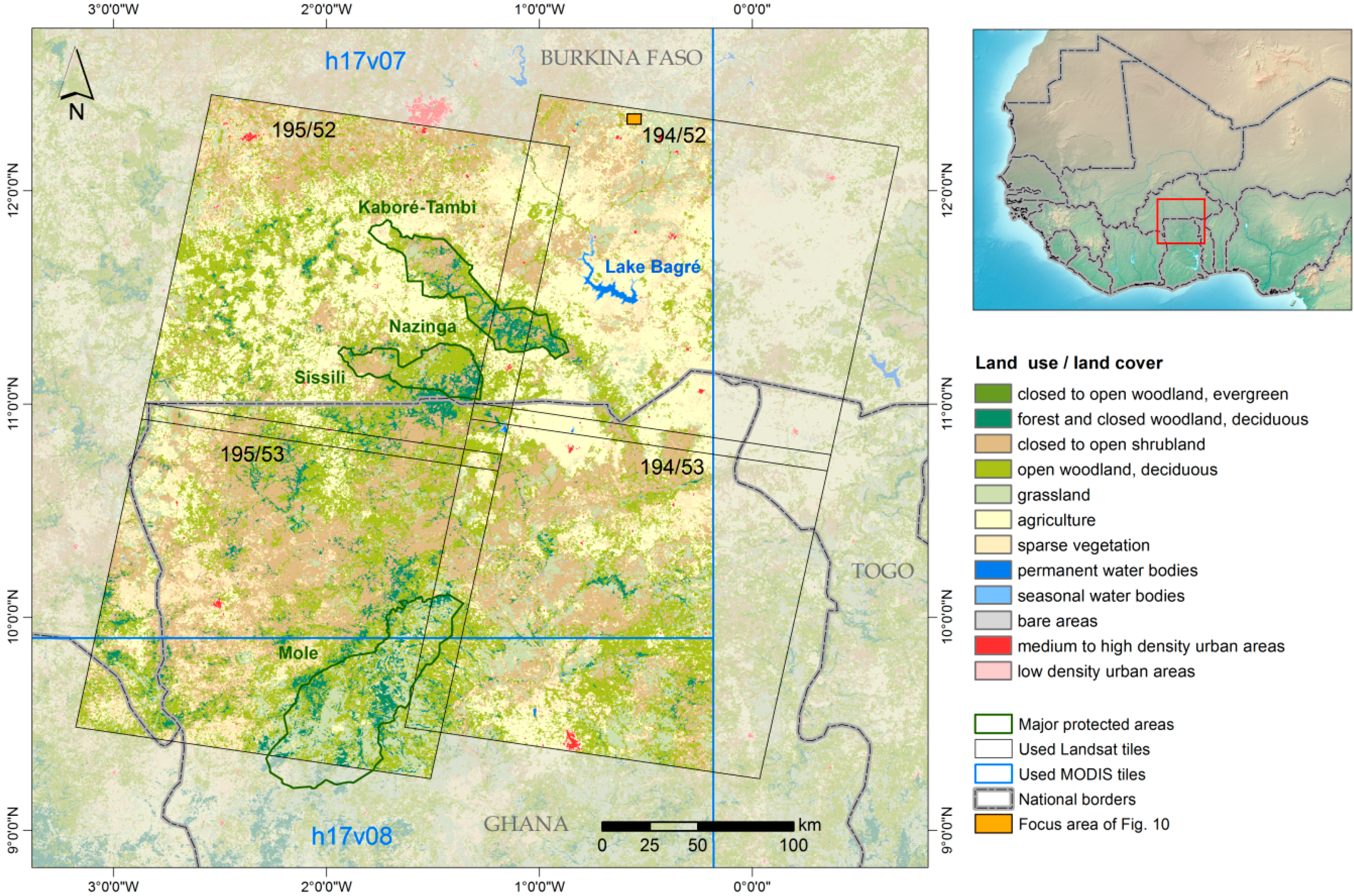
2. Study Area
3. Materials and Methods
3.1. Landsat-8 Operational Land Imager (OLI)
3.2. Terra/Aqua Moderate Resolution Imaging Spectroradiometer (MODIS) MCD43A4, Collection 6
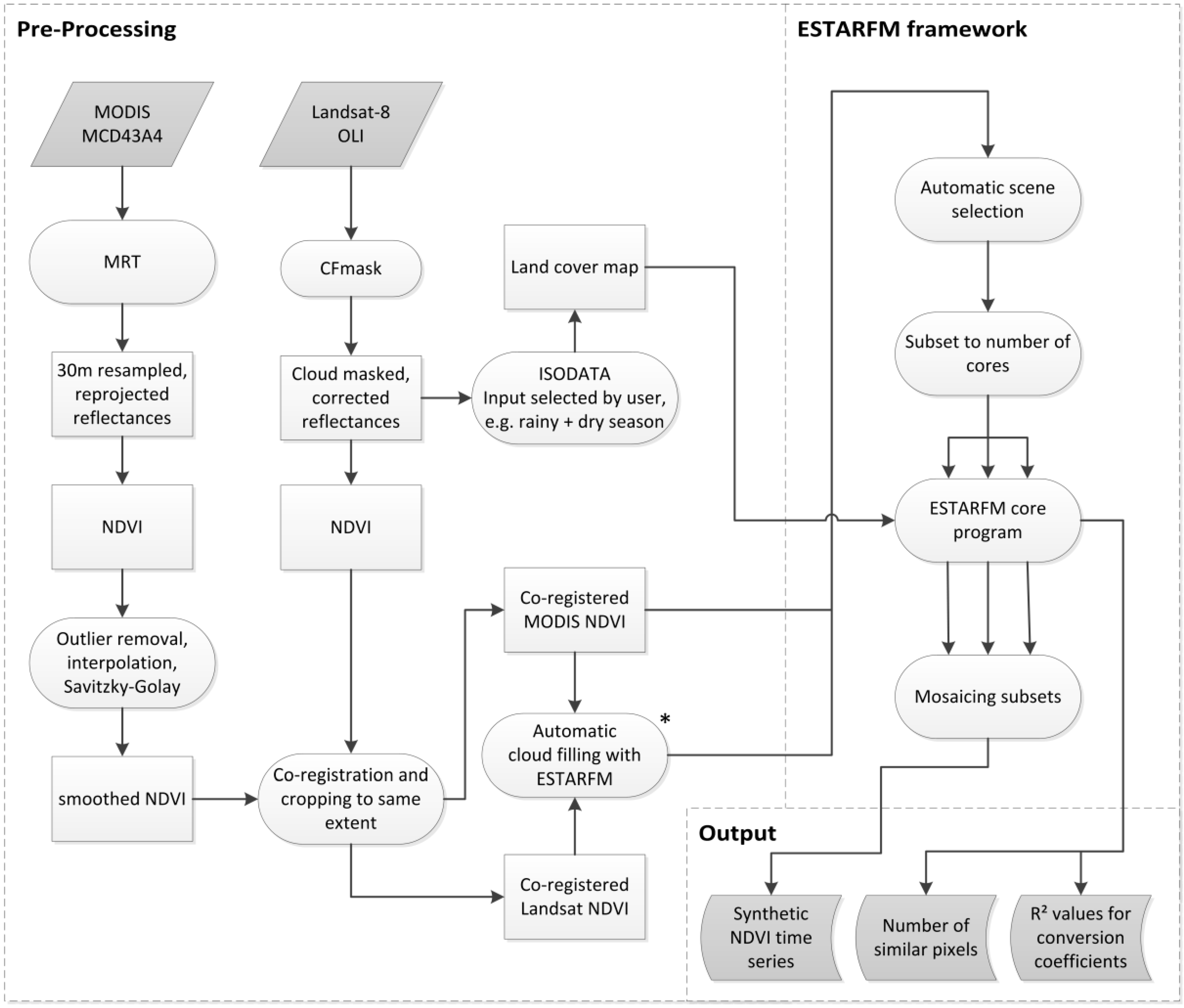
3.3. Method for the Generation of High Temporal Resolution Time Series
3.3.1. Modified Selection of Similar Pixels
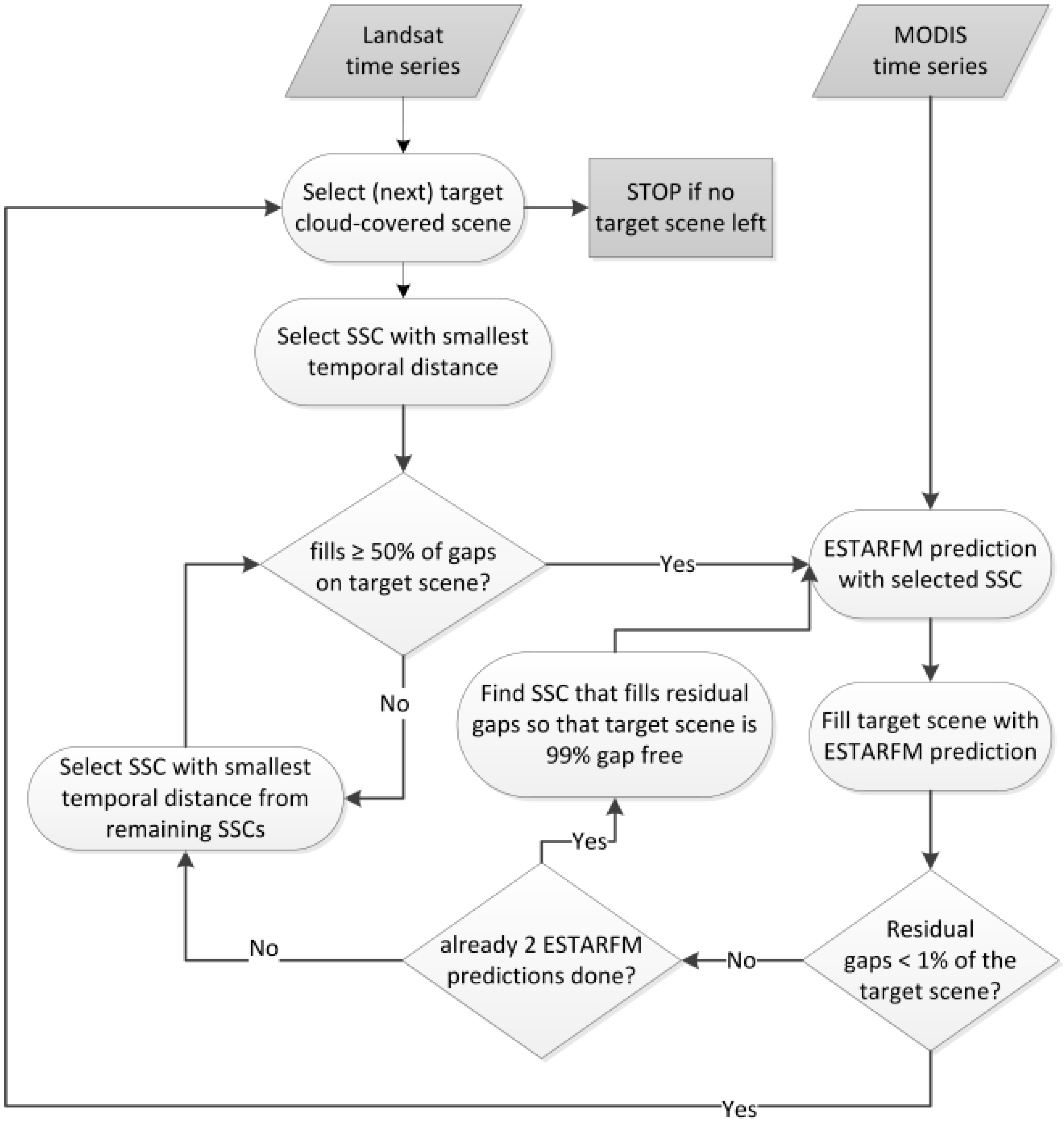
3.3.2. Integration of Cloud-Affected Landsat Scenes
3.3.3. Quality Information
3.3.4. Automation and Improvement of Performance
3.3.5. Application of the Enhance Spatial and Temporal Adaptive Reflectance Fusion Model (ESTARFM) Framework in the Study Area
3.4. Accuracy Assessment
4. Results
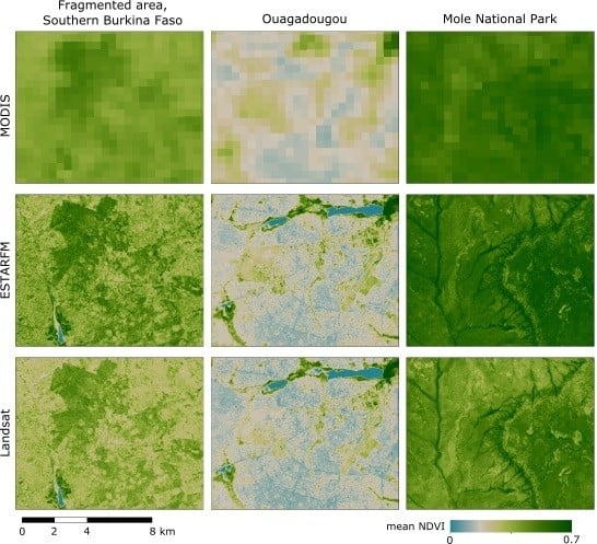
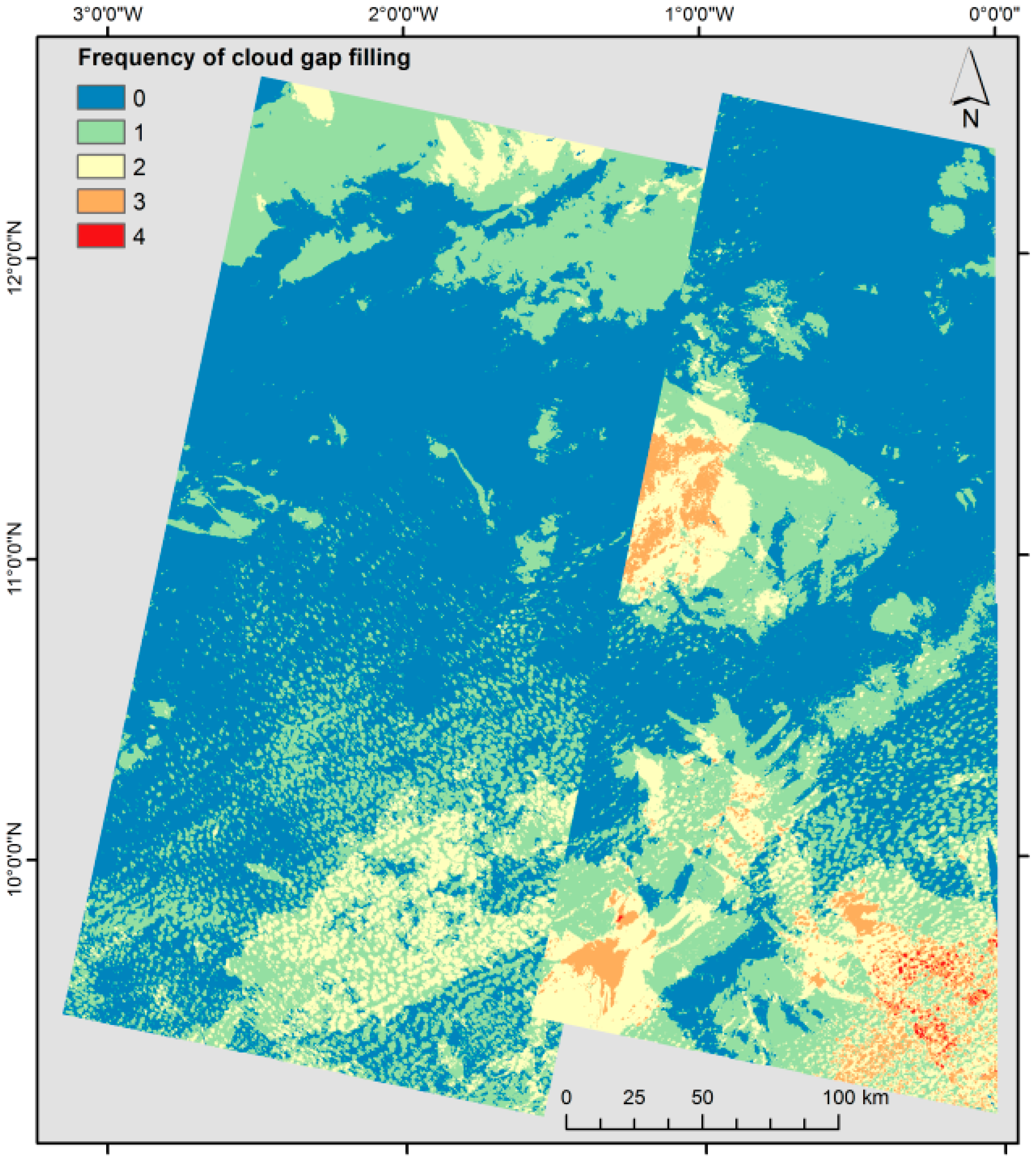
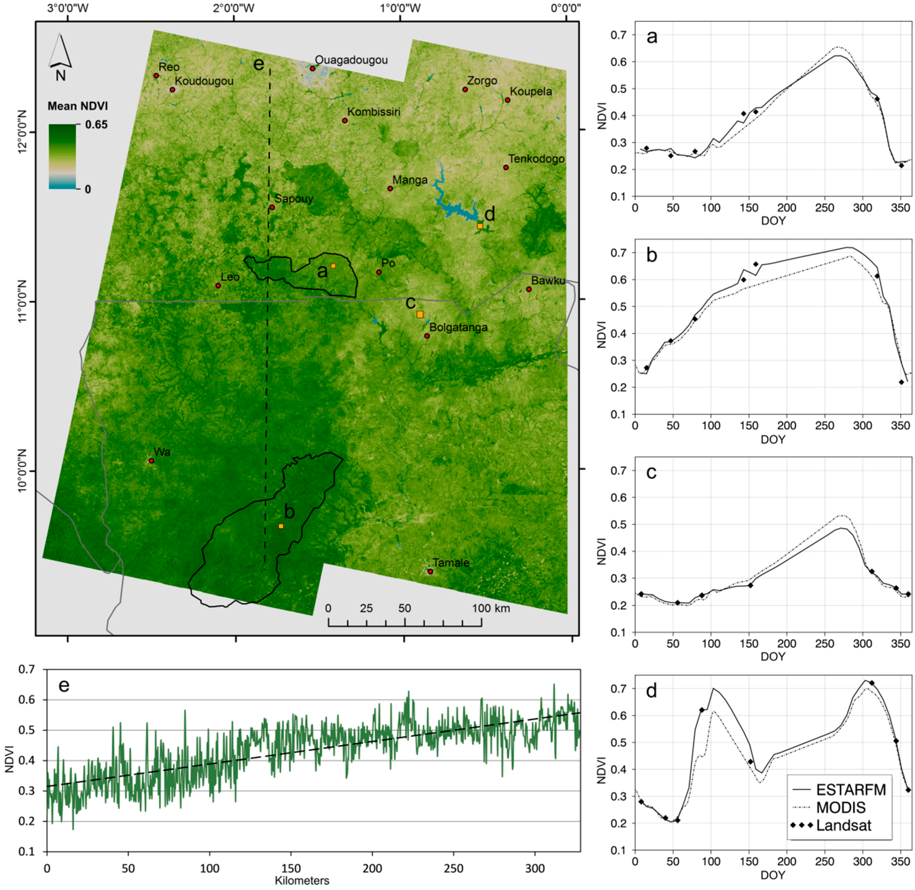
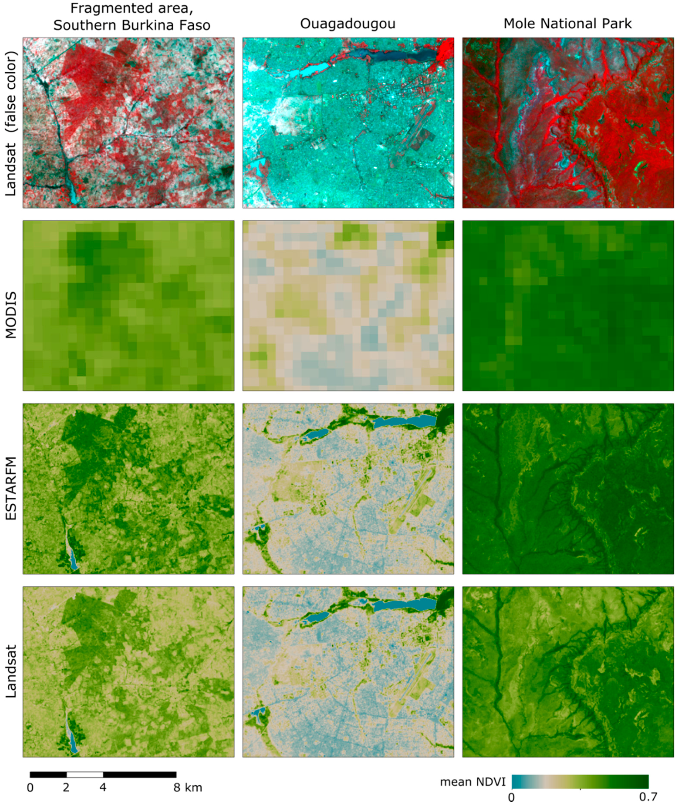
4.1. Spatio-Temporal Patterns of the ESTARFM Time Series
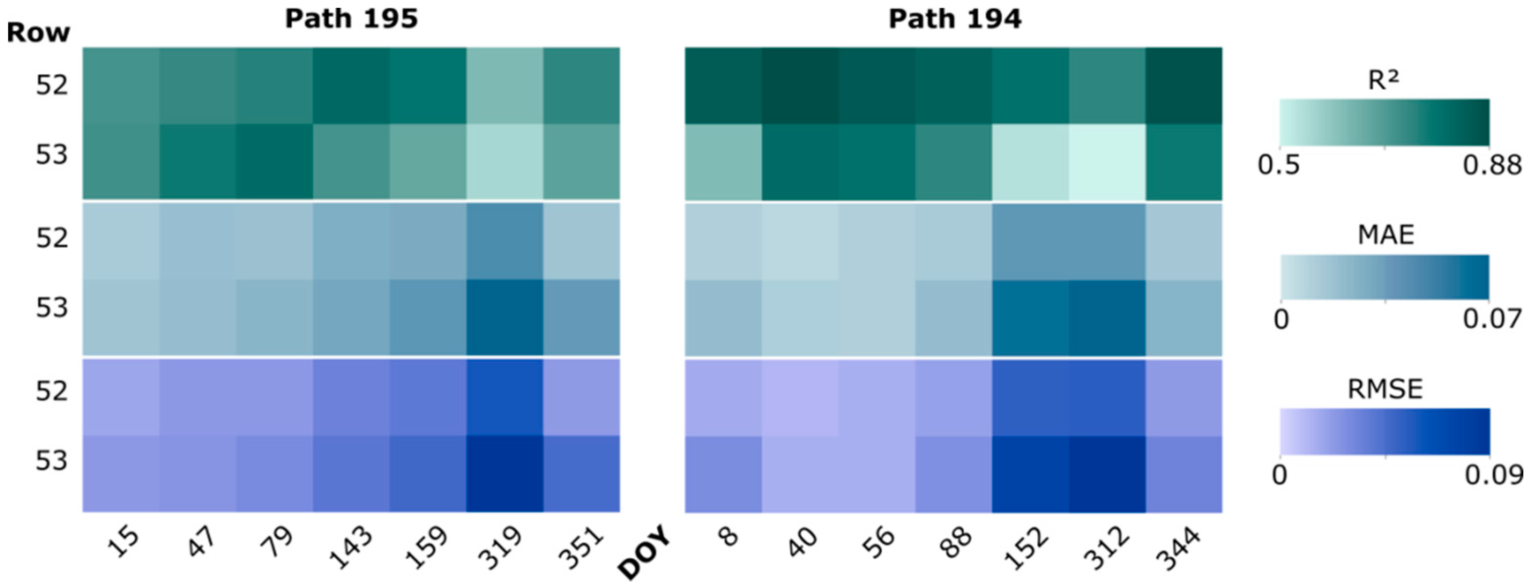
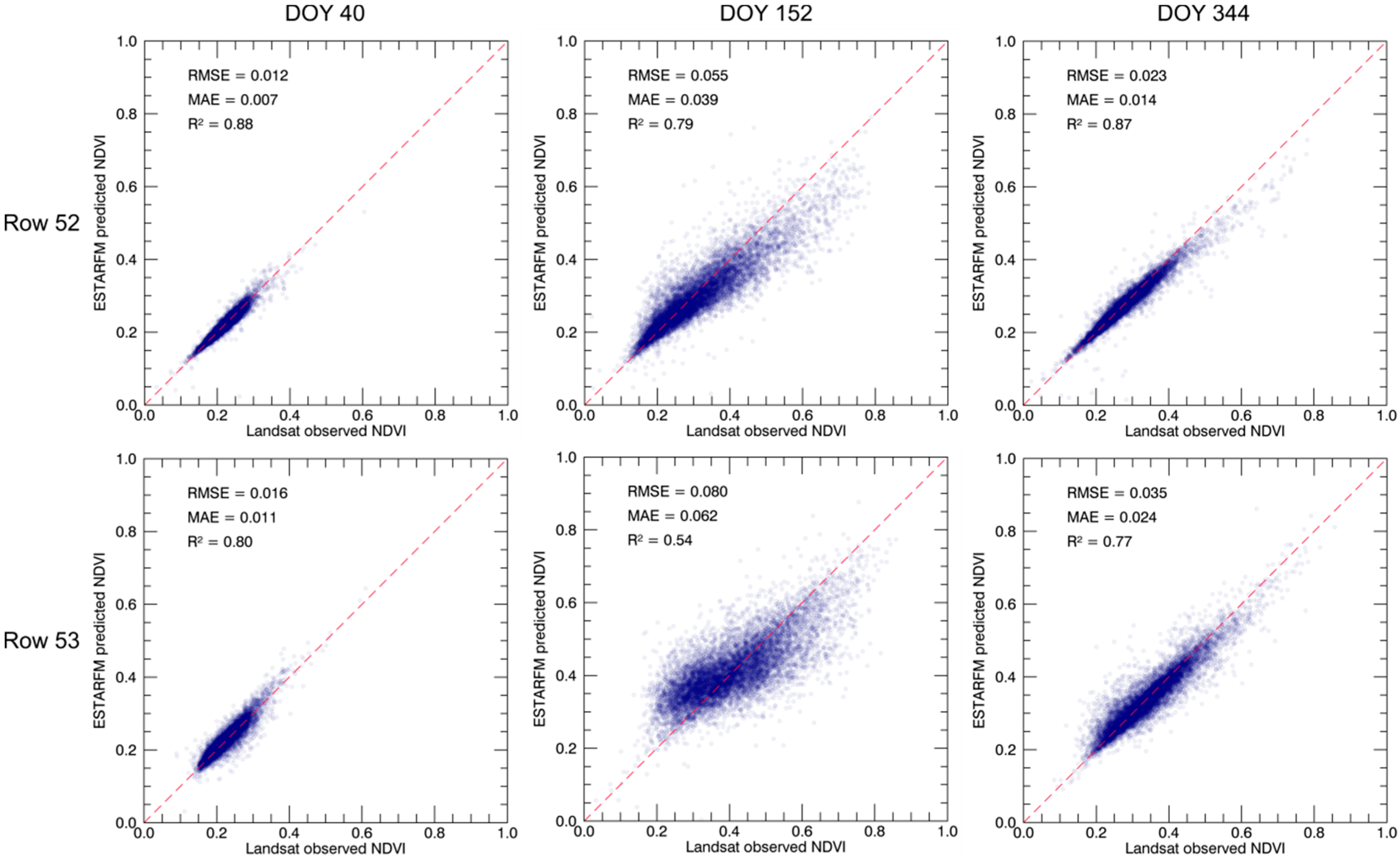
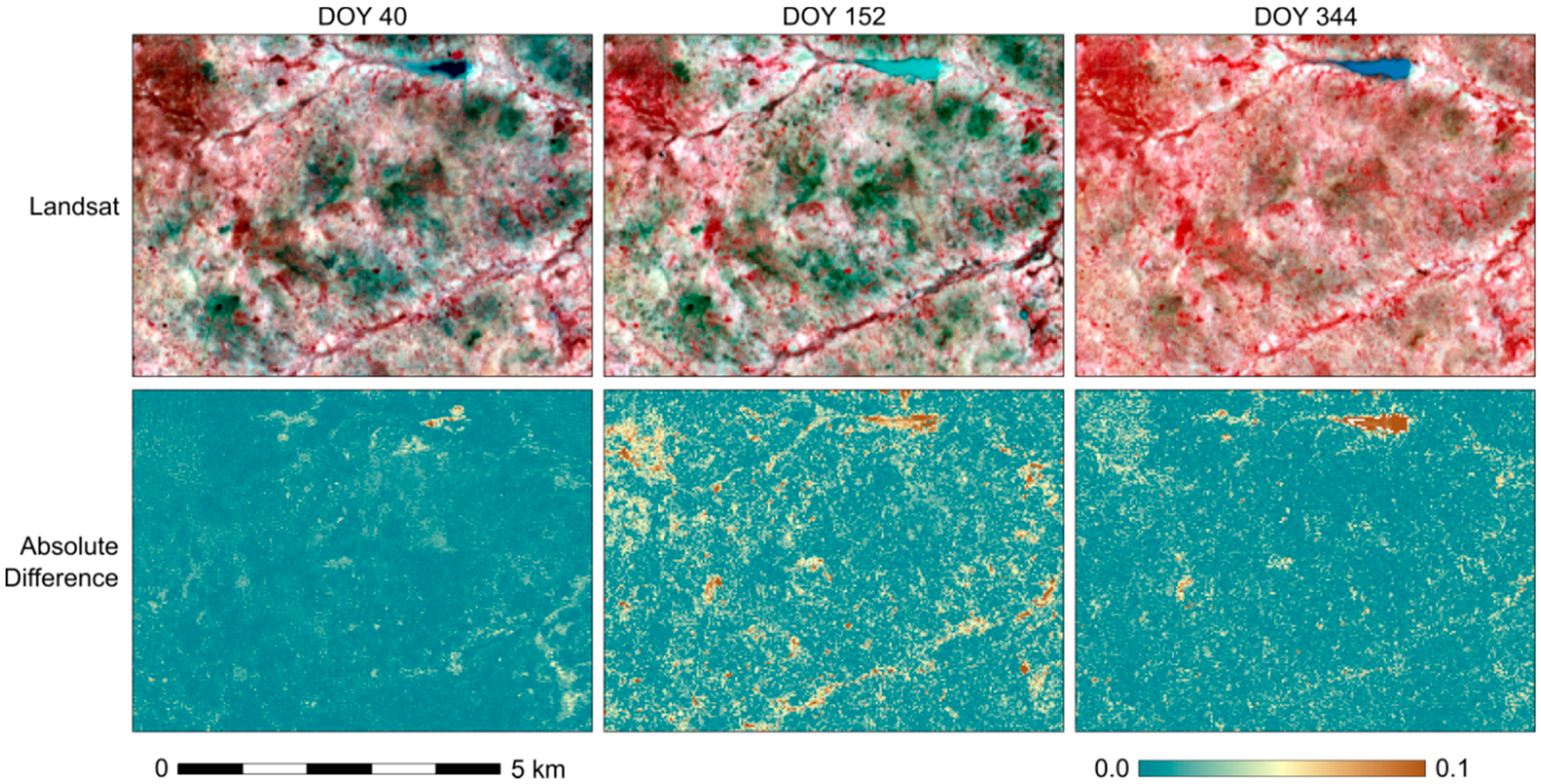
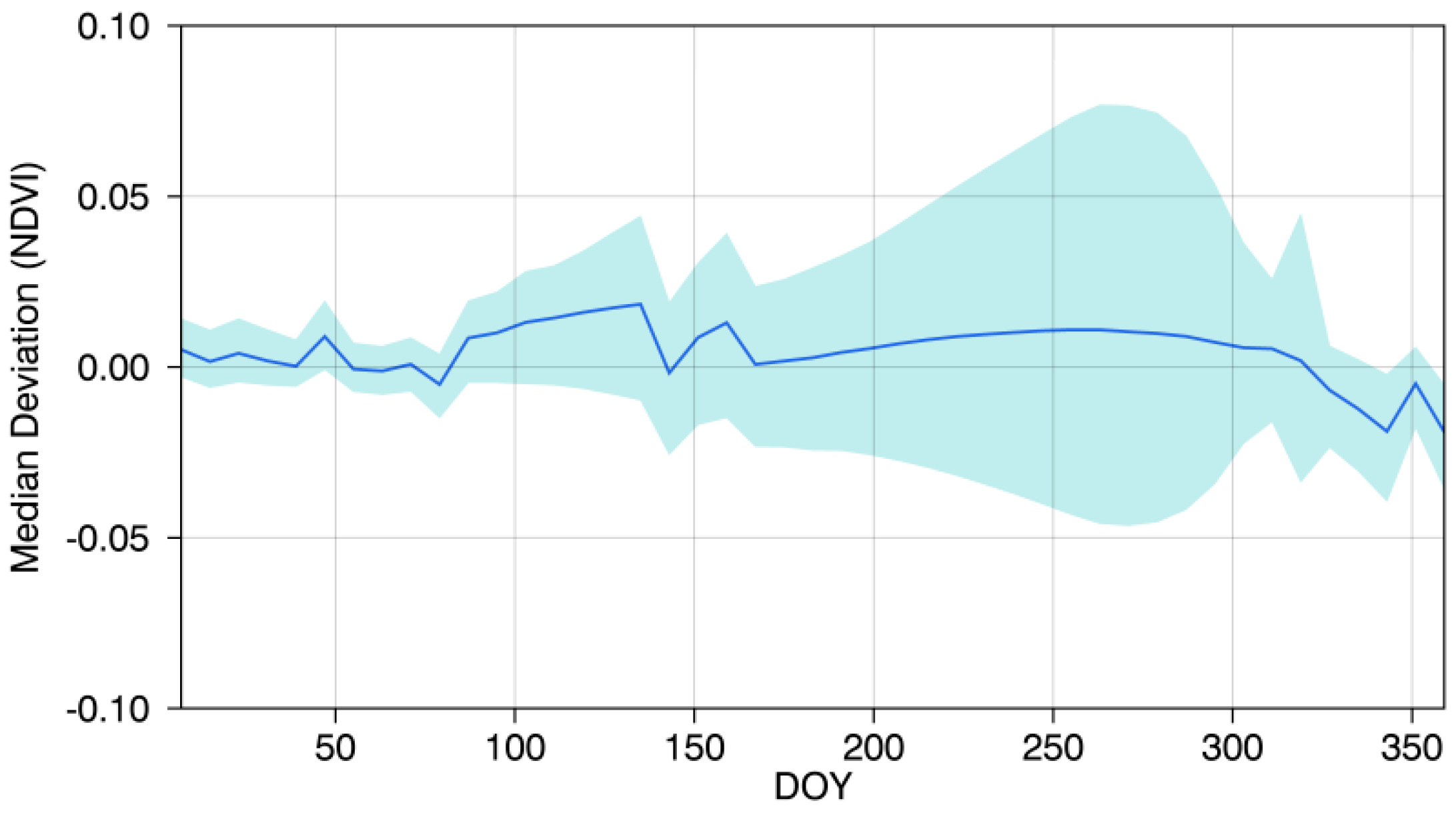
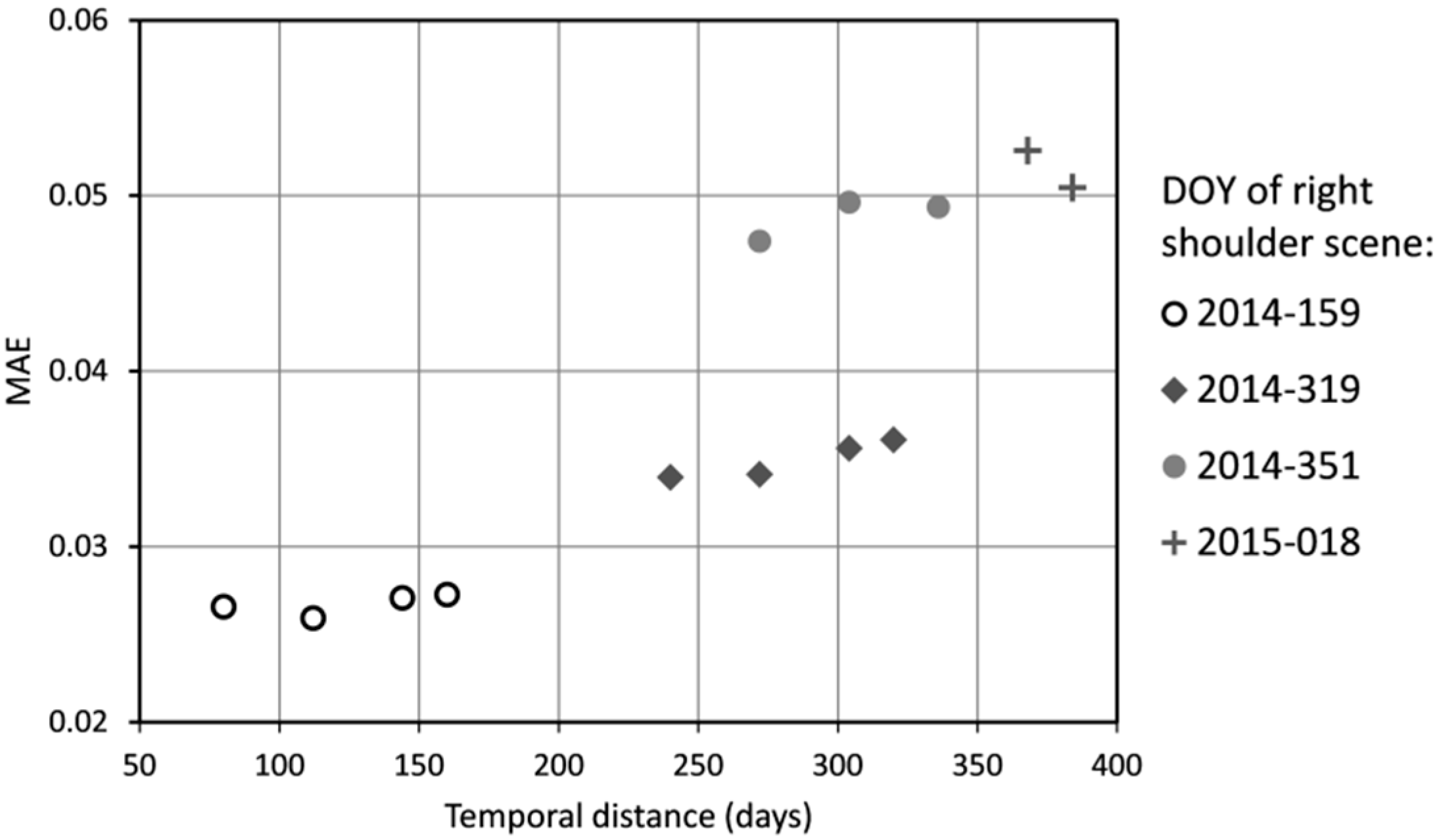
4.2. Accuracy Assessment of the ESTARFM Predictions
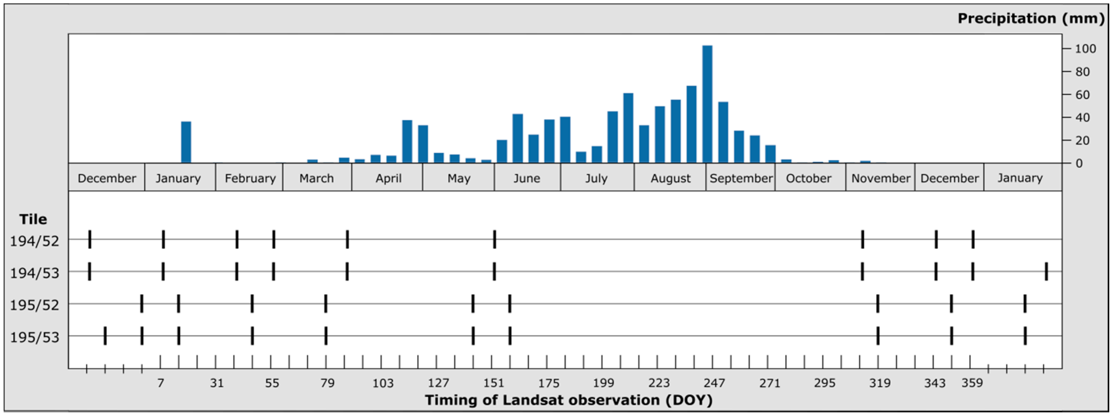
4.3. Input Data Availability and Influence on ESTARFM Predictions
5. Discussion
5.1. Uncertainties in the Prediction with ESTARFM
5.2. Added Value of the ESTARFM Framework for Cloud-Prone Areas
5.3. Added Value of the ESTARFM Framework for Large-Scale Analyses
6. Conclusions and Outlook
Acknowledgments
Author Contributions
Conflicts of Interest
References
- Knauer, K.; Gessner, U.; Dech, S.; Kuenzer, C. Remote sensing of vegetation dynamics in West Africa. Int. J. Remote Sens. 2014, 35, 37–41. [Google Scholar] [CrossRef]
- Gao, F.; Masek, J.G.; Schwaller, M.; Hall, F. On the blending of the Landsat and MODIS surface reflectance: Predicting daily Landsat surface reflectance. IEEE Trans. Geosci. Remote Sens. 2006, 44, 2207–2218. [Google Scholar]
- Zhu, X.; Chen, J.; Gao, F.; Chen, X.; Masek, J.G. An enhanced spatial and temporal adaptive reflectance fusion model for complex heterogeneous regions. Remote Sens. Environ. 2010, 114, 2610–2623. [Google Scholar] [CrossRef]
- Chen, B.; Huang, B.; Xu, B. Comparison of spatiotemporal fusion models: A review. Remote Sens. 2015, 7, 1798–1835. [Google Scholar] [CrossRef]
- Tewes, A.; Thonfeld, F.; Schmidt, M.; Oomen, R.; Zhu, X.; Dubovyk, O.; Menz, G.; Schellberg, J. Using RapidEye and MODIS data fusion to monitor vegetation dynamics in semi-arid rangelands in South Africa. Remote Sens. 2015, 7, 6510–6534. [Google Scholar] [CrossRef]
- Walker, J.; de Beurs, K.; Wynne, R. Phenological response of an Arizona dryland forest to Short-term climatic extremes. Remote Sens. 2015, 7, 10832–10855. [Google Scholar] [CrossRef]
- Doña, C.; Chang, N.-B.; Caselles, V.; Sánchez, J.M.; Camacho, A.; Delegido, J.; Vannah, B.W. Integrated satellite data fusion and mining for monitoring lake water quality status of the Albufera de Valencia in Spain. J. Environ. Manag. 2015, 151, 416–426. [Google Scholar]
- Bisquert, M.; Bégué, A.; Poncelet, P.; Teisseire, M. Evaluation of fusion methods for crop monitoring purposes. In Proceedings of the 2014 IEEE Geoscience and Remote Sensing Symposium, Quebec, QC, Canada, 13–18 July 2014; pp. 1429–1432.
- Emelyanova, I.V.; McVicar, T.R.; van Niel, T.G.; Li, L.T.; van Dijk, A.I.J.M. Assessing the accuracy of blending Landsat-MODIS surface reflectances in two landscapes with contrasting spatial and temporal dynamics: A framework for algorithm selection. Remote Sens. Environ. 2013, 133, 193–209. [Google Scholar] [CrossRef]
- Jarihani, A.; McVicar, T.; Van Niel, T.; Emelyanova, I.; Callow, J.; Johansen, K. Blending Landsat and MODIS data to generate multispectral indices: A comparison of “Index-then-Blend” and “Blend-then-Index” approaches. Remote Sens. 2014, 6, 9213–9238. [Google Scholar] [CrossRef] [Green Version]
- Gao, F.; Wang, P.; Masek, J. Integrating remote sensing data from multiple optical sensors for ecological and crop condition monitoring. Proc. SPIE 2013, 8869. [Google Scholar] [CrossRef]
- Schmidt, M.; Lucas, R.; Bunting, P.; Verbesselt, J.; Armston, J. Multi-resolution time series imagery for forest disturbance and regrowth monitoring in Queensland, Australia. Remote Sens. Environ. 2015, 158, 156–168. [Google Scholar] [CrossRef] [Green Version]
- Verbesselt, J.; Hyndman, R.; Newnham, G.; Culvenor, D. Detecting trend and seasonal changes in satellite image time series. Remote Sens. Environ. 2010, 114, 106–115. [Google Scholar] [CrossRef]
- Zhang, F.; Zhu, X.; Liu, D. Blending MODIS and Landsat images for urban flood mapping. Int. J. Remote Sens. 2014, 35, 3237–3253. [Google Scholar] [CrossRef]
- Olson, D.M.; Dinerstein, E.; Wikramanayake, E.D.; Burgess, N.D.; Powell, G.V.N.; Underwood, E.C.; D’amico, J.A.; Itoua, I.; Strand, H.E.; Morrison, J.C.; et al. Terrestrial ecoregions of the world: A new map of life on earth. Bioscience 2001, 51, 933–938. [Google Scholar] [CrossRef]
- Gessner, U.; Knauer, K.; Kuenzer, C.; Dech, S. Land surface phenology in a west African savanna: Impact of land use, land cover and fire. In Remote Sensing Time Series; Kuenzer, C., Dech, S., Wagner, W., Eds.; Springer International Publishing: Berlin, Germany; Heidelberg, Germany, 2015; pp. 203–223. [Google Scholar]
- FAO FAOSTAT. Available online: http://faostat3.fao.org/faostat-gateway/go/to/home/E (accessed on 13 May 2016).
- Forkuor, G. Agricultural Land Use Mapping in West Africa Using Multi-sensor Satellite Imagery; University of Wuerzburg: Wuerzburg, Germany, 2014. [Google Scholar]
- Gessner, U.; Machwitz, M.; Esch, T.; Tillack, A.; Naeimi, V.; Kuenzer, C.; Dech, S. Multi-sensor mapping of West African land cover using MODIS, ASAR and TanDEM-X/TerraSAR-X data. Remote Sens. Environ. 2015, 164, 282–297. [Google Scholar] [CrossRef]
- USGS Landsat Data Access. Available online: http://landsat.usgs.gov/Landsat_Search_and_Download.php (accessed on 3 December 2015).
- USGS. Product Guide—Provisional Landsat 8 Surface Reflectance Product; Department of the Interior USA Geological Survey: Reston, VA, USA, 2016.
- Zhu, Z.; Woodcock, C.E. Object-based cloud and cloud shadow detection in Landsat imagery. Remote Sens. Environ. 2012, 118, 83–94. [Google Scholar] [CrossRef]
- Bliefernicht, J.; Kunstmann, H.; Hingerl, L.; Rummler, T.; Andresen, S.; Mauder, M.; Steinbrecher, R.; Frieß, R.; Gochis, D.; Gessner, U.; et al. Field and simulation experiments for investigating regional land-atmosphere interactions in West Africa: Experimental setup and first results. Clim. Land Surf. Chang. Hydrol. 2013, 359, 226–232. [Google Scholar]
- Quansah, E.; Mauder, M.; Balogun, A.A.; Amekudzi, L.K.; Hingerl, L.; Bliefernicht, J.; Kunstmann, H. Carbon dioxide fluxes from contrasting ecosystems in the Sudanian Savanna in West Africa. Carbon Balance Manag. 2015, 10, 1–17. [Google Scholar] [CrossRef] [PubMed]
- Professor Crystal Schaaf’s Lab MODIS User Guide V006. Available online: https://www.umb.edu/spectralmass/terra_aqua_modis/v006 (accessed on 14 March 2016).
- LP DAAC MODIS Reprojection Tool. Available online: https://lpdaac.usgs.gov/tools/modis_reprojection_tool (accessed on 3 December 2015).
- Eklundh, L.; Jönsson, P. TIMESAT 3.2 with Parallel Processing Software Manual; Lund University: Lund, Sweden, 2015. [Google Scholar]
- Savitzky, A.; Golay, M.J.E. Smoothing and differentiation of data by simplified least squares procedures. Anal. Chem. 1964, 36, 1627–1639. [Google Scholar] [CrossRef]
- Tou, J.T.; Gonzalez, R.C. Pattern Recognition Principles; NASA: Washington, DC, USA, 1974.
- Tian, F.; Wang, Y.; Fensholt, R.; Wang, K.; Zhang, L.; Huang, Y. Mapping and evaluation of NDVI trends from synthetic time series obtained by blending Landsat and MODIS data around a coalfield on the loess plateau. Remote Sens. 2013, 5, 4255–4279. [Google Scholar] [CrossRef]
- Fu, D.; Chen, B.; Wang, J.; Zhu, X.; Hilker, T. An improved image fusion approach based on enhanced spatial and temporal the adaptive reflectance fusion model. Remote Sens. 2013, 5, 6346–6360. [Google Scholar] [CrossRef]
- Gao, F.; Hilker, T.; Zhu, X.; Anderson, M.; Masek, J.; Wang, P.; Yang, Y. Fusing Landsat and MODIS data for vegetation monitoring. IEEE Geosci. Remote Sens. Mag. 2015, 3, 47–60. [Google Scholar] [CrossRef]
- Walker, J.J.; de Beurs, K.M.; Wynne, R.H. Dryland vegetation phenology across an elevation gradient in Arizona, USA, investigated with fused MODIS and Landsat data. Remote Sens. Environ. 2014, 144, 85–97. [Google Scholar] [CrossRef]
- Zhu, X.; Helmer, E.H.; Gao, F.; Liu, D.; Chen, J.; Lefsky, M.A. A flexible spatiotemporal method for fusing satellite images with different resolutions. Remote Sens. Environ. 2016, 172, 165–177. [Google Scholar] [CrossRef]
- Walker, J.J.; de Beurs, K.M.; Wynne, R.H.; Gao, F. Evaluation of Landsat and MODIS data fusion products for analysis of dryland forest phenology. Remote Sens. Environ. 2012, 117, 381–393. [Google Scholar] [CrossRef]
- Fensholt, R.; Sandholt, I.; Proud, S.R.; Stisen, S.; Rasmussen, M.O. Assessment of MODIS sun-sensor geometry variations effect on observed NDVI using MSG SEVIRI geostationary data. Int. J. Remote Sens. 2010, 31, 6163–6187. [Google Scholar] [CrossRef]
- Bréon, F.M.; Vermote, E. Correction of MODIS surface reflectance time series for BRDF effects. Remote Sens. Environ. 2012, 125, 1–9. [Google Scholar] [CrossRef]
- Fensholt, R.; Anyamba, A.; Stisen, S.; Sandholt, I.; Pak, E.; Small, J. Comparisons of compositing period length for vegetation index data from polar-orbiting and geostationary satellites for the cloud-prone region of West Africa. Photogramm. Eng. Remote Sens. 2007, 73, 297–309. [Google Scholar] [CrossRef]
- Brandt, M.; Mbow, C.; Diouf, A.A.; Verger, A.; Samimi, C.; Fensholt, R. Ground- and satellite-based evidence of the biophysical mechanisms behind the greening Sahel. Glob. Chang. Biol. 2015, 21, 1610–1620. [Google Scholar] [CrossRef] [PubMed]
- Fensholt, R.; Rasmussen, K.; Kaspersen, P.S.; Huber, S.; Horion, S.; Swinnen, E. Assessing land degradation/recovery in the African Sahel from long-term earth observation based primary productivity and precipitation relationships. Remote Sens. 2013, 5, 664–686. [Google Scholar] [CrossRef] [Green Version]
- Leroux, L.; Jolivot, A.; Bégué, A.; Seen, D.; Zoungrana, B. How reliable is the MODIS land cover product for crop mapping sub-saharan agricultural landscapes? Remote Sens. 2014, 6, 8541–8564. [Google Scholar] [CrossRef] [Green Version]
- Vintrou, E.; Desbrosse, A.; Bégué, A.; Traoré, S.; Baron, C.; lo Seen, D. Crop area mapping in West Africa using landscape stratification of MODIS time series and comparison with existing global land products. Int. J. Appl. Earth Observ. Geoinf. 2012, 14, 83–93. [Google Scholar] [CrossRef]


| Input | Original ESTARFM | ESTARFM Framework (9 Cores) |
|---|---|---|
| 4 bands | 24 h 49 min | 4 h 38 min |
| NDVI | 15 h 32 min | 1 h 45 min |
| Row | DOY 191 | DOY 271 | DOY 287 | DOY 303 | ||||||||
|---|---|---|---|---|---|---|---|---|---|---|---|---|
| MAE | RMSE | R2 | MAE | RMSE | R2 | MAE | RMSE | R2 | MAE | RMSE | R2 | |
| 52 | 0.05 | 0.07 | 0.74 | 0.10 | 0.12 | 0.41 | 0.07 | 0.10 | 0.53 | 0.03 | 0.05 | 0.76 |
| 53 | 0.06 | 0.07 | 0.58 | 0.07 | 0.09 | 0.30 | 0.06 | 0.08 | 0.33 | 0.05 | 0.06 | 0.56 |
© 2016 by the authors; licensee MDPI, Basel, Switzerland. This article is an open access article distributed under the terms and conditions of the Creative Commons Attribution (CC-BY) license (http://creativecommons.org/licenses/by/4.0/).
Share and Cite
Knauer, K.; Gessner, U.; Fensholt, R.; Kuenzer, C. An ESTARFM Fusion Framework for the Generation of Large-Scale Time Series in Cloud-Prone and Heterogeneous Landscapes. Remote Sens. 2016, 8, 425. https://0-doi-org.brum.beds.ac.uk/10.3390/rs8050425
Knauer K, Gessner U, Fensholt R, Kuenzer C. An ESTARFM Fusion Framework for the Generation of Large-Scale Time Series in Cloud-Prone and Heterogeneous Landscapes. Remote Sensing. 2016; 8(5):425. https://0-doi-org.brum.beds.ac.uk/10.3390/rs8050425
Chicago/Turabian StyleKnauer, Kim, Ursula Gessner, Rasmus Fensholt, and Claudia Kuenzer. 2016. "An ESTARFM Fusion Framework for the Generation of Large-Scale Time Series in Cloud-Prone and Heterogeneous Landscapes" Remote Sensing 8, no. 5: 425. https://0-doi-org.brum.beds.ac.uk/10.3390/rs8050425