Production of the Japan 30-m Land Cover Map of 2013–2015 Using a Random Forests-Based Feature Optimization Approach

Abstract

Achieving more timely, accurate and transparent information on the distribution and dynamics of the world’s land cover is essential to understanding the fundamental characteristics, processes and threats associated with human-nature-climate interactions. Higher resolution (~30–50 m) land cover mapping is expected to advance the understanding of the multi-dimensional interactions of the human-nature-climate system with the potentiality of representing most of the biophysical processes and characteristics of the land surface. However, mapping at 30-m resolution is complicated with existing manual techniques, due to the laborious procedures involved with the analysis and interpretation of huge volumes of satellite data. To cope with this problem, an automated technique was explored for the production of a high resolution land cover map at a national scale. The automated technique consists of the construction of a reference library by the optimum combination of the spectral, textural and topographic features and predicting the results using the optimum random forests model. The feature-rich reference library-driven automated technique was used to produce the Japan 30-m resolution land cover (JpLC-30) map of 2013–2015. The JpLC-30 map consists of seven major land cover types: water bodies, deciduous forests, evergreen forests, croplands, bare lands, built-up areas and herbaceous. The resultant JpLC-30 map was compared to the existing 50-m resolution JAXA High Resolution Land-Use and Land-Cover (JHR LULC) map with reference to Google Earth™ images. The JpLC-30 map provides more accurate and up-to-date land cover information than the JHR LULC map. This research recommends an effective utilization of the spectral, textural and topographic information to increase the accuracy of automated land cover mapping.

1. Introduction

Land cover and land use change is a paramount global environmental issue. Achieving more timely, accurate and transparent information on the distribution and dynamics of the world’s land cover is essential to understand the fundamental characteristics, processes and threats associated with human-nature-climate interactions, including, among others, biogeochemical and hydrological cycles, biodiversity and genetic variations, land degradation and environmental pollution, climate change and poverty, globalization and sustainability and environmental scarcity and societal conflicts. Higher resolution (~30–50 m) land cover mapping is expected to advance the understanding of the multi-dimensional interactions of the human-nature-climate system with the potentiality of representing most of the biophysical processes and characteristics of the surface of the Earth required for environmental conservation and management, hydro-climatic characterization and modeling and ensuring crop insurance and food security.

Dramatic alteration of the Earth’s land surface by human activities has caused significant impact on the atmospheric carbon budget, chemical fluxes, fresh water and biodiversity; resulting in a human-dominated planet [1,2]. Local changes in land use driven by increased human requirements of food, fiber, water and shelter have accelerated energy, water and fertilizer consumption; undermining the capacity of ecosystems to sustain food production and biodiversity and to regulate climate and air quality; challenging the capacity of the biosphere to provide goods and services in the long term [3]. Understanding the dynamics of land cover and land use is crucial to address theory, concepts, models and applications relevant to socio-environmental problems [4]. The Earth system and society’s use of ecological resources are tightly coupled through exchanges of water, energy and nutrients. However, land cover conversion, cultivation of favorable species and the transfer of organisms between locations are the primary interfaces between human society and the Earth system [5]. Both natural and anthropogenic land use change can substantially impact global air quality with significant radiative effects on global and local climate [6] and even pollinators necessary for maintaining plant communities [7].

Land cover is also an important variable required for the arena of socio-environmental studies, such as climate change analysis [8,9,10,11], carbon cycle modeling [12,13,14,15], habitat and biodiversity studies [16,17] and public health [18]. In spite of the wider applicability of the land cover information, scientific understanding of the distribution and dynamics of land use and land cover change is limited [19]. A number of global land cover maps are available mostly at moderate spatial resolution (~500 m), such as Moderate Resolution Imaging Spectroradiometer (MODIS) Land Cover Type product (MCD12Q1 2012; [20]) and Global Land Cover by National Mapping Organizations (GLCNMO 2008; [21]), as some examples. Apart from multi-class land cover maps, a number of individual class maps are also produced at a global scale, for example agricultural lands [22,23], water bodies [24,25], urban and built-up areas [26,27], inundation areas [28] and forest cover [29,30].

Moderate resolution maps have limited ability to discriminate mixed classes (mixed pixels effect) characterized by a mosaic of trees, shrubs and herbaceous vegetation [31]. Moreover, existing global datasets have considerable disagreements and uncertainties across the regional or continental level [32]. A comparison of classification schemes of different maps has shown many inconsistencies between the definition of map classes; and the classification scheme and validation methodology have contributed the highest error [33]. Meta-analysis of hundreds of land-cover mapping research works has concluded that more spectral bands or a combination of data types resulted in increased mapping accuracies, whereas the complexity of a classification scheme decreases the overall accuracy [34]. A review of 23 global and 41 regional land cover products has emphasized the need for international coordination and harmonization initiatives for compatible land cover product generation [35]. Higher resolution (~30–50 m) land cover characterization and monitoring permit the detection of land change at the scale of most human activities and offer the increased flexibility of environmental model parameterization needed for global change studies [36]. Recently, there have been some efforts in the production of high-resolution land cover maps at national, regional and global scales.

In the United States, a partnership of 10 federal agencies has provided a 30-m resolution land cover map of the year 2011 [37,38,39]. It is based on Landsat Thematic Mapper (TM) and Enhanced TM plus (ETM+) imagery, Digital Elevation Model (DEM) and Defense Meteorological Satellite Program (DMSP) Operational Linescan System (OLS)-based nighttime light data. The eighteen land cover types classified by the NLCD 2011 product are comprised of open water, perennial snow/ice, four types of urban areas, barren land, deciduous forest, evergreen forest, mixed forest, shrub/scrub, grassland/herbaceous, pasture/hay, cultivated cropland, woody wetlands and herbaceous wetlands.

The National Administration of Surveying, Mapping and Geo-information (NASG) of China has produced a 30-m resolution Global Land Cover data Product (GlobeLand30) of the year 2010 by using multispectral data from Landsat TM, ETM+, the China Environmental Disaster Alleviation Satellite (HJ-1A/B) and various auxiliary data, such as existing land cover maps, MODIS Normalized Difference Vegetation Index (NDVI) data and global DEM data. The GlobeLand30 has classified ten land cover types, namely cultivated land, forest, grassland, shrub land, wetlands, water bodies, tundra, artificial surfaces, bare land and permanent snow/ice. It utilizes the integration of pixel- and object-based classification approaches, integration of reference data and knowledge-based verification procedures. It is a hierarchical classification strategy accompanied by a rule-based workflow [40].

Giri and Long [41] produced Landsat-based high-resolution land cover map of South America for the year 2010 by using decision tree classification based on NDVI and the Shuttle Radar Topography Mission (SRTM) DEM data. They mapped only five discrete land cover classes: trees, open water, barren, perennial snow/ice and other vegetation.

In Japan, the Japan Aerospace Exploration Agency (JAXA) has produced the JAXA High Resolution Land-Use and Land-Cover map (JHR LULC map) using multi-year (2006–2011) optical data acquired from the Advanced Visible and Near-Infrared Radiometer Type 2 (AVNIR-2), Panchromatic Remote-sensing Instrument for Stereo Mapping (PRISM)-based DEM data, The Advanced Land Observing Satellite (ALOS) Phased Array type L-band Synthetic Aperture Radar (PALSAR)-based Synthetic Aperture Radar (SAR) mosaic data, Terra/MODIS-based NDVI data and transportation network data from the Geospatial Information Authority of Japan (GSI). It provides nine categorical land cover classes at ~50-m spatial resolution, mainly based on the decision tree method [42]. The nine land cover types classified by the JHR LULC map are water, urban, paddy, crops, grass, deciduous forest, evergreen forest, bare land and snow/ice.

Higher resolution land cover mapping is relevant to Japan because of the rapid pace of land use/cover changes. The wider topographic variation of Japan has supported all of the sub-tropical, warm-temperate, cool-temperate and boreal vegetation types; and Japan has maintained a stagnant forest cover over the last century. However, land cover and land use in Japan are no exception to urban and industrial development; yet more prone to damages from earthquakes, tsunamis and volcanoes; and likely to be susceptible to disaster-induced evacuation, out-migration and an aging society. Himiyama [43] analyzed land use/cover changes in Japan over the last hundred years; and projected that paddy-field is the largest type of land use that will have suffered from urban expansion by the 2020s in central Japan. Harada et al. [44] have described that despite the overall increase of forest cover from 72.1% in 1900 to 76.9% in 2001, in many areas, the climax of vegetation has been replaced by secondary forests, such as conifer timber plantations, especially in the warm and mid-temperate zones of western Japan. Tracking of higher resolution land use/cover changes in Japan is also expected to contribute to anthropogenic carbon reduction strategies and the maintenance of biological diversity and ecological processes.

However, available techniques on higher resolution land cover mapping as used by the existing maps at local, regional and global scales involve labor-intensive and massively time-consuming procedures. On the other hand, a very low accuracy ranging from 53.88% (maximum likelihood classifier) to 64.89% (support vector machine) has been reported from a fully-automated classification of the 30-m resolution global land cover mapping [45]. Due to complexities associated with the handling, analysis and interpretation of a huge volume of satellite and ancillary data, the production of a more timely land cover map is very cumbersome with the existing knowledge-based workflow and manual procedures. This paper presents an automated approach for the production of a 30-m resolution land cover map at a national scale by optimizing the combination of multi-spectral, multi-textural and topographic features, all obtained from satellites.

2. Methodology

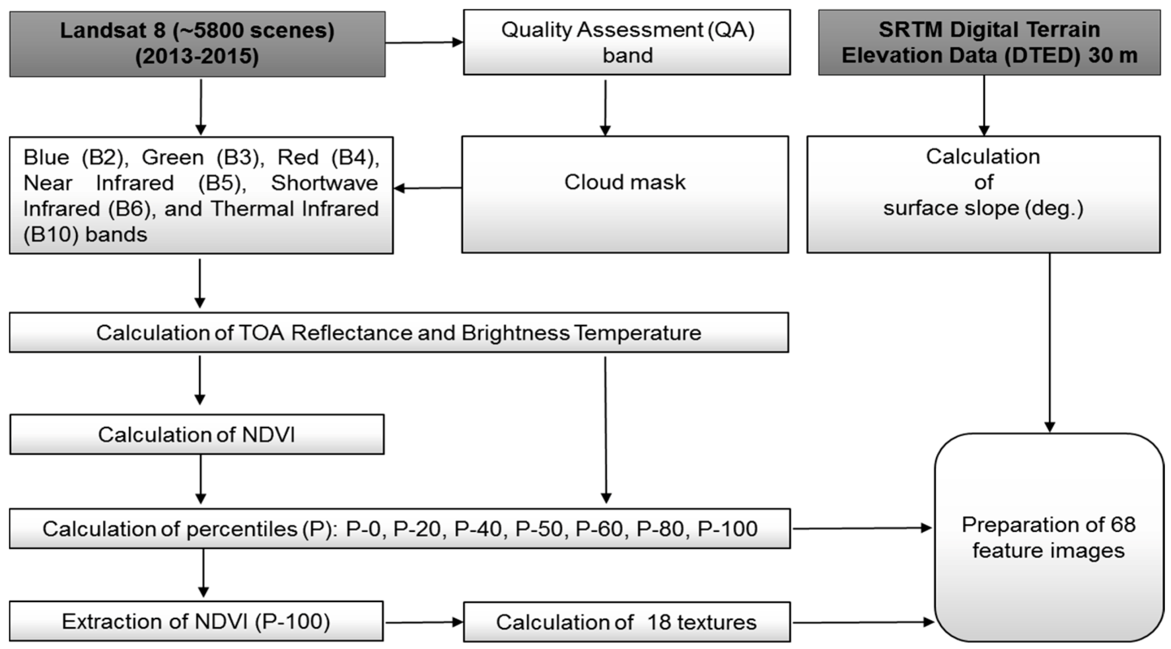
2.1. Processing of Satellite Data

All of the ~5800 standard terrain corrected (Level 1T) Landsat 8 Operational Land Imager (OLI) and Thermal Infrared Sensor (TIRS) scenes of 2013–2015 available from the United States Geological Survey (USGS) over Japan were processed. Landsat-8 has been monitoring global land surface since its launch on 11 February 2013 with a standard 16-day repeat cycle [46,47]. Quantized and calibrated scaled Digital Numbers (DNs) for each OLI and TIRS band delivered as 16-bit unsigned integers were converted into Top-Of-Atmosphere (TOA) spectral reflectance and brightness temperature (K) values using the rescaling coefficients found in the metadata file. Out of nine OLS and two TIRS bands of the Landsat 8 data, seven bands (blue, green, red, near infrared, shortwave infrared and thermal infrared) were extracted. The clouds were removed by using separate Quality Assessment (QA) band information available in the Landsat 8 data. Void data are a great nuisance for pipelining the machine learning and prediction procedures. Hence, the percentile-based image compositing technique was preferred over time period-based (such as monthly) composting techniques to avoid the void data resulting from the latter technique. Using all multi-temporal data of 2013–2015, multiple percentiles, 0, 20, 40, 50, 60, 80 and 100, were calculated pixel by pixel for each band to capture the temporal information of the land cover. In addition, the Normalized Difference Vegetation Index (NDVI; [48]) was calculated for each scene, and similarly, multiple NDVI percentiles, 0, 20, 40, 50, 60, 80 and 100, were calculated pixel by pixel. The temporal distribution of the NDVI data ranging between −1 and 1 varies with the land cover type. Therefore, a percentile, for instance the 40th percentile NDVI (the statistical value below which 40 percent of the multi-temporal NDVI data are found), also varies with the cover types. Using maximum NDVI (100th percentile) images, 18 types of image textures [49,50] were also calculated. The gray-level co-occurrence matrix (GLCM) functions implemented in OTB (https://www.orfeo-toolbox.org/), an open-source C++ library for image processing, were used to calculate the image textures using a 3 × 3 sliding window size with a single pixel offset. The maximum NDVI image representing the growing season signal of the vegetation was deliberately chosen to obtain drastic textural contrast between the vegetation and non-vegetation cover types. In this way, a stack of 67 feature images (~175 gigabytes) was prepared by exploiting a huge volume (~5 terabytes) of Landsat 8 data. In addition, land surface slope data were prepared from 30-m resolution SRTM-based Digital Terrain Elevation Data (DTED) available from the USGS. The satellite data were automatically processed through custom programming deployed for large-scale remote sensing applications. The processing steps involved in the preparation of feature images are shown in Figure 1. In machine learning, a feature is an individual measurable property of a phenomenon being observed [51].

Altogether, 68 feature images were used as an input dataset in the research. Feature images are also listed in

Table 1. List of spectral, textural and topographic feature images used in the research. DTED, Digital Terrain Elevation Data.

	Spectral	Textural	Topographic	Temporal	No. of Features
Landsat 8	Blue, Green, Red, Near Infrared, Shortwave Infrared, and Thermal Infrared	-	-	7	42
	NDVI	-	-	7	7
	NDVI (Max.)	Energy, Entropy, Sum Entropy, Difference Entropy, Sum Correlation, Maximal Correlation, Sum Variance, Difference Variance, Sum Squares Variance Homogeneity, Dissimilarity, Inertia, Measures of Correlation-1and 2, Contrast, Cluster Shade, and Prominence	-	-	18
SRTM DTED	-	-	Slope	-	1

.

2.2. Collection of Reference Data

The JpLC-30 map includes seven land cover types, namely water bodies, deciduous forests, evergreen forests, croplands, bare lands, built-up areas and herbaceous. The classification scheme is described as follows:

• Croplands land used for cultivated crops, such as paddy fields, irrigated or dry farmland and vegetables.
• Deciduous forests: land covered with trees, with vegetation cover over 30%, including broadleaf and coniferous forests, and sparse woodland, with cover of 10%–30%, that shed their leaves seasonally.
• Evergreen forests: land covered with trees, with vegetation cover over 30%, including broadleaf and coniferous forests, and sparse woodland with cover of 10%–30% that maintain leaves throughout the year.
• Herbaceous: land covered with vegetation, as grass or herbs, with cover over 10%.
• Water bodies: water bodies within the land area, including rivers, lakes, reservoirs and ponds.
• Built-up areas: land modified by human activities, including all kinds of impervious surfaces.
• Bare lands: land with vegetation cover lower than 10%, including sandy fields and bare rocks.

Approximately 100 polygons belonging to each land cover class as defined above were collected based on reference data and expert knowledge. The seasonal true-color (RGB) composite images prepared from Landsat 8 data and Google Earth ™-based time-lapse images were used to collect reference data. Reference polygons were collected by interactively viewing all seasonal RGB images and Google Earth™ images available for 2013–2015. Reference polygons were collected only from large homogenous areas that could be interpreted visually. Out of ~100 polygons for each land cover class, 22,500 geo-location points distributed at least 50 m apart and located inside the reference polygons were extracted randomly and used as the training data. Similarly, another set of ~50 polygons belonging to each class were also collected separately, and 7500 geo-location points for each class were used as the validation data. The distribution of 30,000 geo-location points belonging to each cover class are displayed in Figure 2.

2.3. Construction of the Reference Library

It should be noted that the reference (training and validation) data are geo-located points that are sensitive to the biophysical changes of the land surface. They cannot be used after a few months or years, since land cover may have changed considerably at that time. Therefore, altogether 210,000 reference points (30,000 points × 7 classes) prepared through visual interpretation and local knowledge were converted into a reference library with the support of 68 feature images (Table 1) prepared in the research. Both reference points and feature images were recorded during the same time period, i.e., 2013–2015. The input of a large number of feature images is expected to represent spectral, textural and topographic variation of the land cover types. The reference library constructed in this way was used to automate the mapping procedure. The spectral, textural and topographic information used for constructing the reference library is the standard measurements obtained from TOA reflectance, TOA brightness temperature and Digital Terrain Model (DTM) data, respectively. However, the spectral, textural and topographic characteristics of the land cover types in other geographical regions may vary significantly. Therefore, the constructed reference library is applicable to repeat monitoring of land cover dynamics of the same region it represents. The reference library includes seven major land cover types present in Japan.

2.4. Machine Learning and Prediction

The land cover exhibits wider spectral variation with respect to both space and time. To discriminate highly dynamic land cover and land use types efficiently, not only temporal variability of the multi-spectral data, but a robust classification algorithm is also required. Random forests [52,53] is a powerful machine learning classifier. Accurate land cover classification and better performance of the random forests model have been described by many researchers [54,55,56,57]. The random forests classifier uses bootstrap aggregating (bagging) to form an ensemble of trees by searching random subspaces from the given data (features) and the best splitting of the nodes by minimizing the correlation between the trees.

The reference library constructed in the research was used to yield an optimum random forests model by choosing the best features. The reference library is a collection of two subsets of data: training and validation data. The hierarchy of best features provided by the random forests model while running with the training data was grouped into 1–68 sets of best features. For each set of best features, the confusion matrix was computed with the validation data. The first set of best features includes only one feature, whereas the last set of best features includes all 68 features. The optimum features defined as the set of the lowest number of input features yielding the highest overall accuracy was selected. The optimum set of features chosen in this way was used to produce the JpLC-30 map in the research. The retrieval of optimum features not only extracts the best features required for discriminating the variability of land cover types, but also reduces the computational cost required for the production of the classification result. The random forests algorithm implemented in OpenCV (http://opencv.org/), an optimized C/C++ programming library for computer vision, machine learning and robotics, was exploited for the production of the JpLC-30 map.

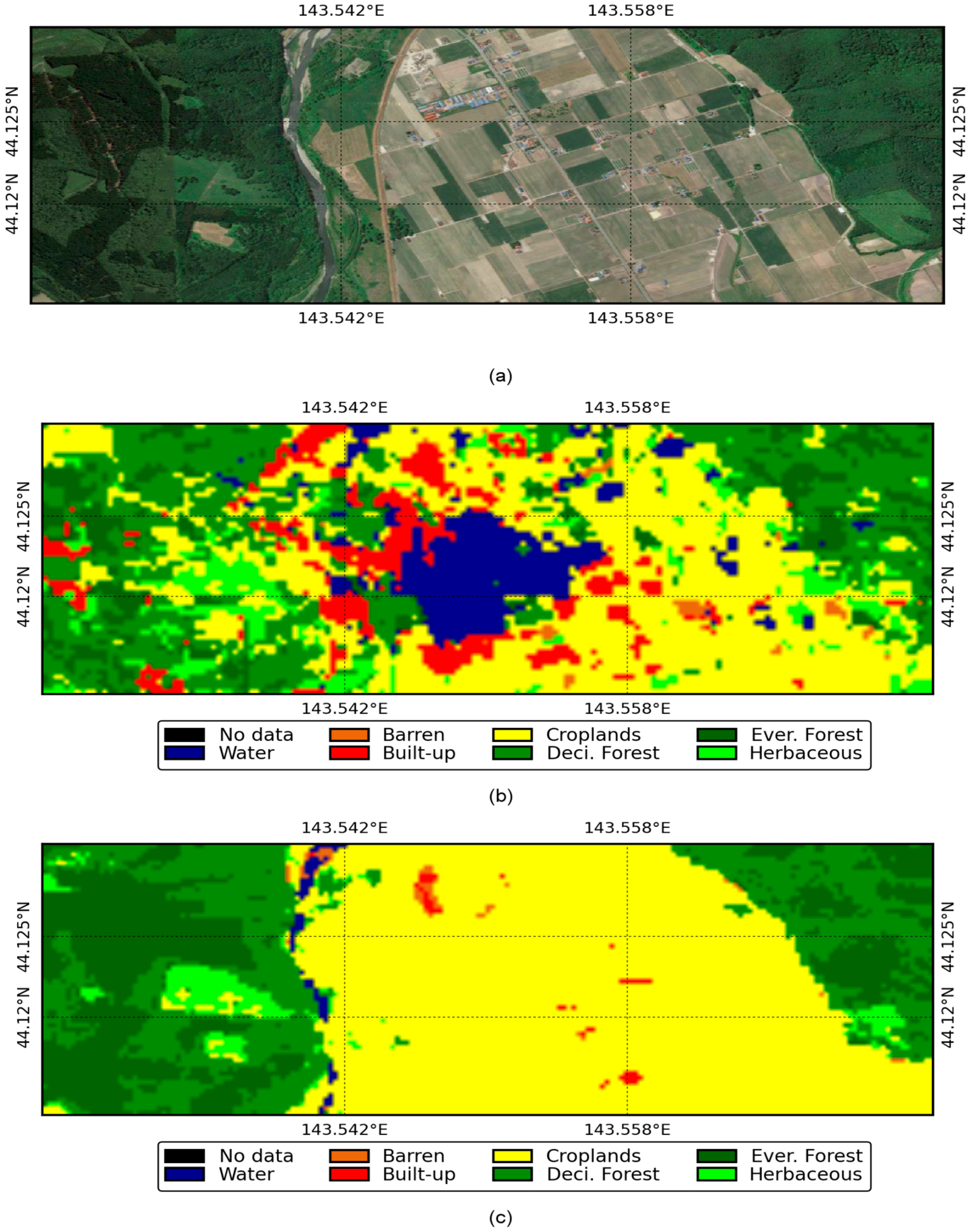
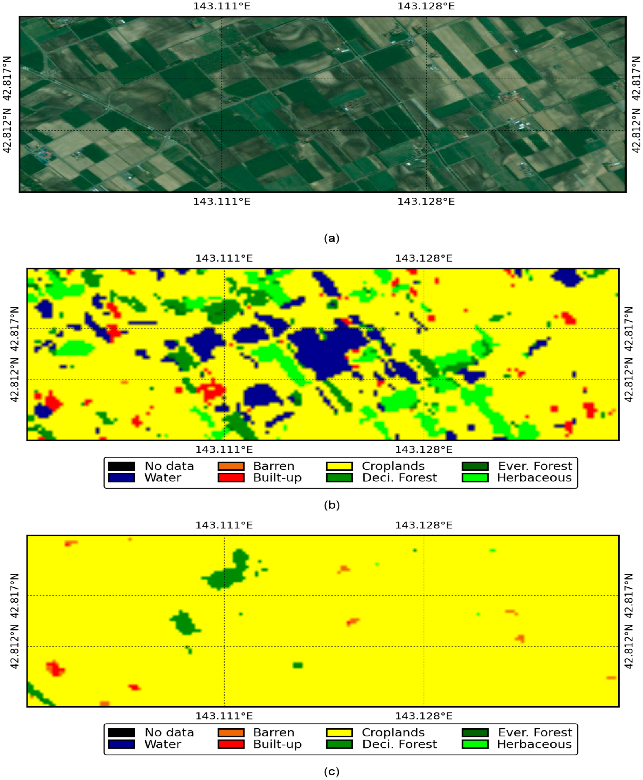
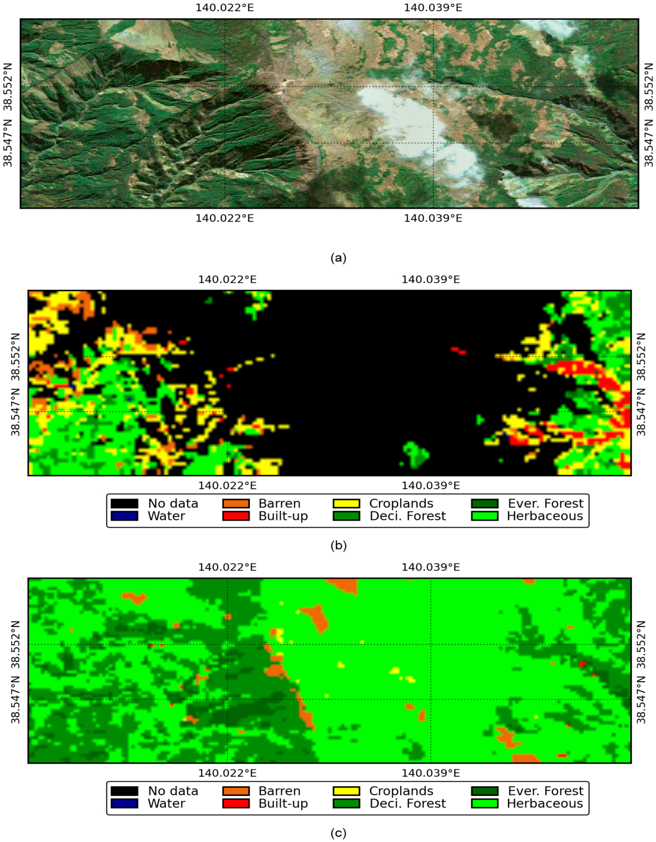
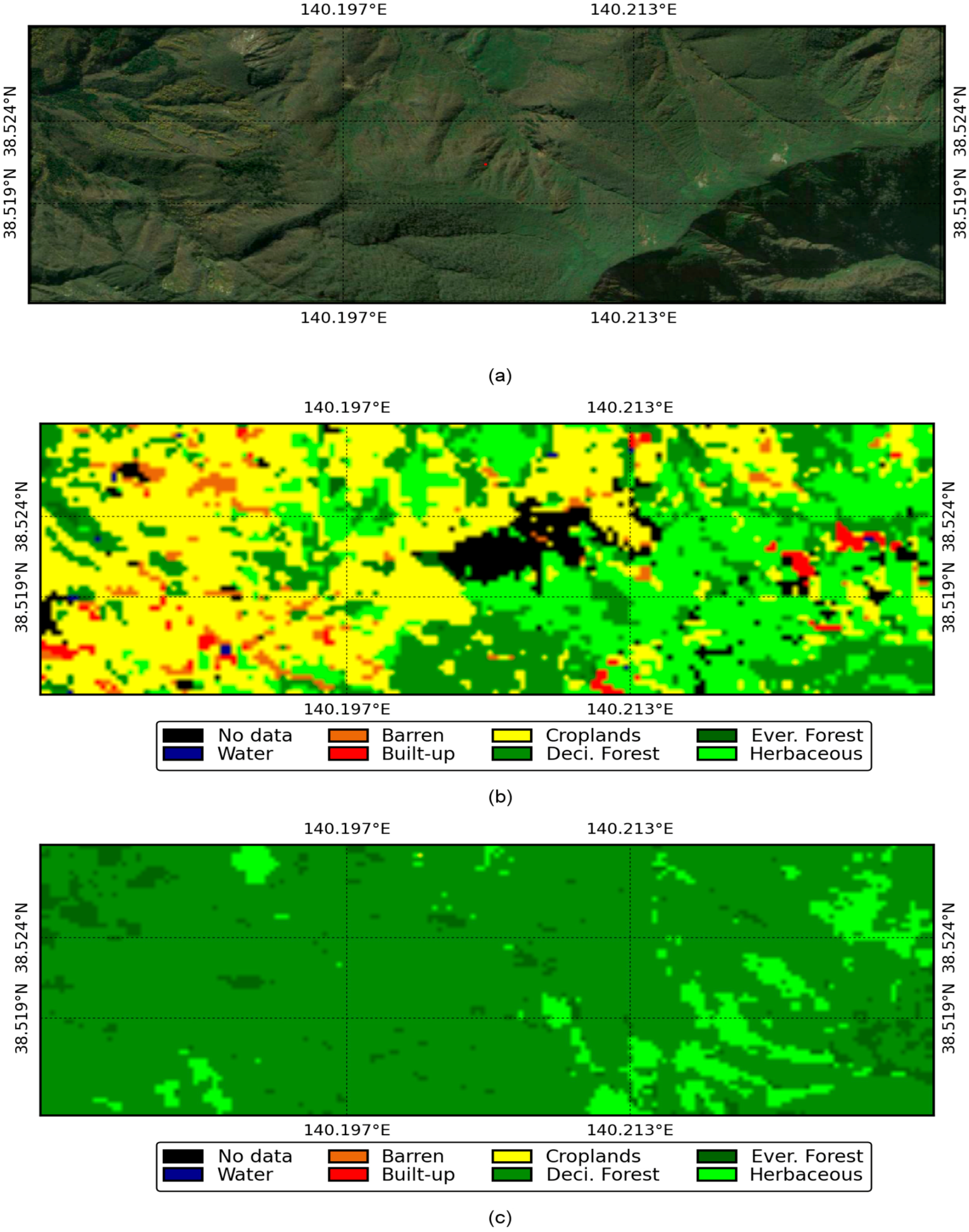
3. Results and Discussion

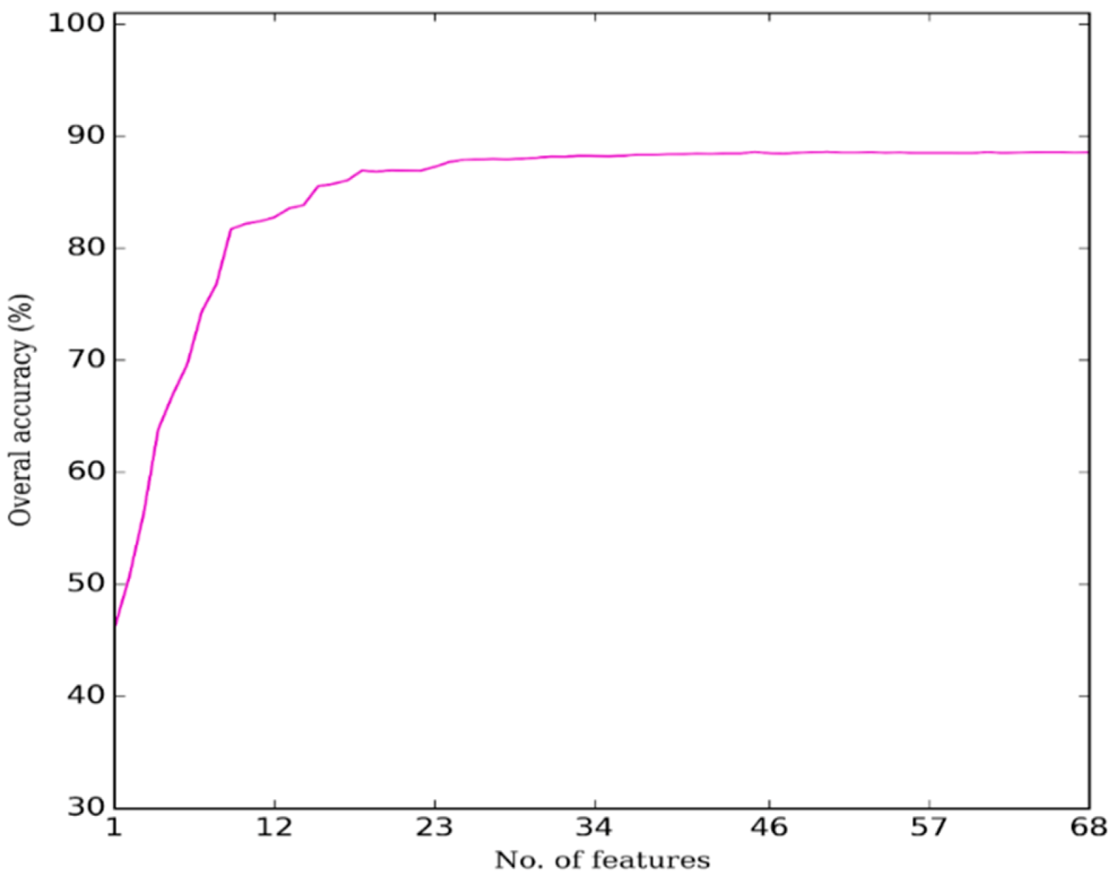
3.1. Selection of Optimum Features

The variation of confusion matrix-based overall accuracy (%) with respect to the number of features used during random forests-based classification of land cover types is demonstrated in Figure 3. The overall accuracy (%) started to elevate with the increase of input features until reaching an optimum point, after which it saturated.

Furthermore, a variation of the confusion matrix with respect to the number of features used is shown in Figure 4. The overall accuracy (%) achieved by using the maximum number of input features (i.e., 68 features) was 88.58% (Figure 4f); whereas the overall accuracy (%) achieved by using 45 features was 88.62% (Figure 4e).

This analysis suggested that out of 68 features, 45 features are sufficient for explaining the variability of land cover types. A lower number of features (i.e., 1–5 features) has resulted in very low accuracy mainly due to the poor discriminability of some classes, which are spectrally indifferent with respect to other classes. For example, as shown in Figure 4a, the built-up and barren classes and croplands and the herbaceous classes were not classified efficiently using a single feature only. The discrimination of land cover types started to increase with the increase of the number of best features used until 45 features were reached. Higher discrimination (overall accuracy = 88.62%) with the selection of 45 features is demonstrated in Figure 4e. After that, the increase of the number of best features did not improve the discrimination with the saturation of the overall accuracy. The optimum set of 45 features selected in this way was used to produce the JpLC-30 map.

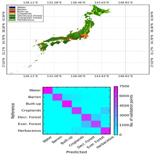
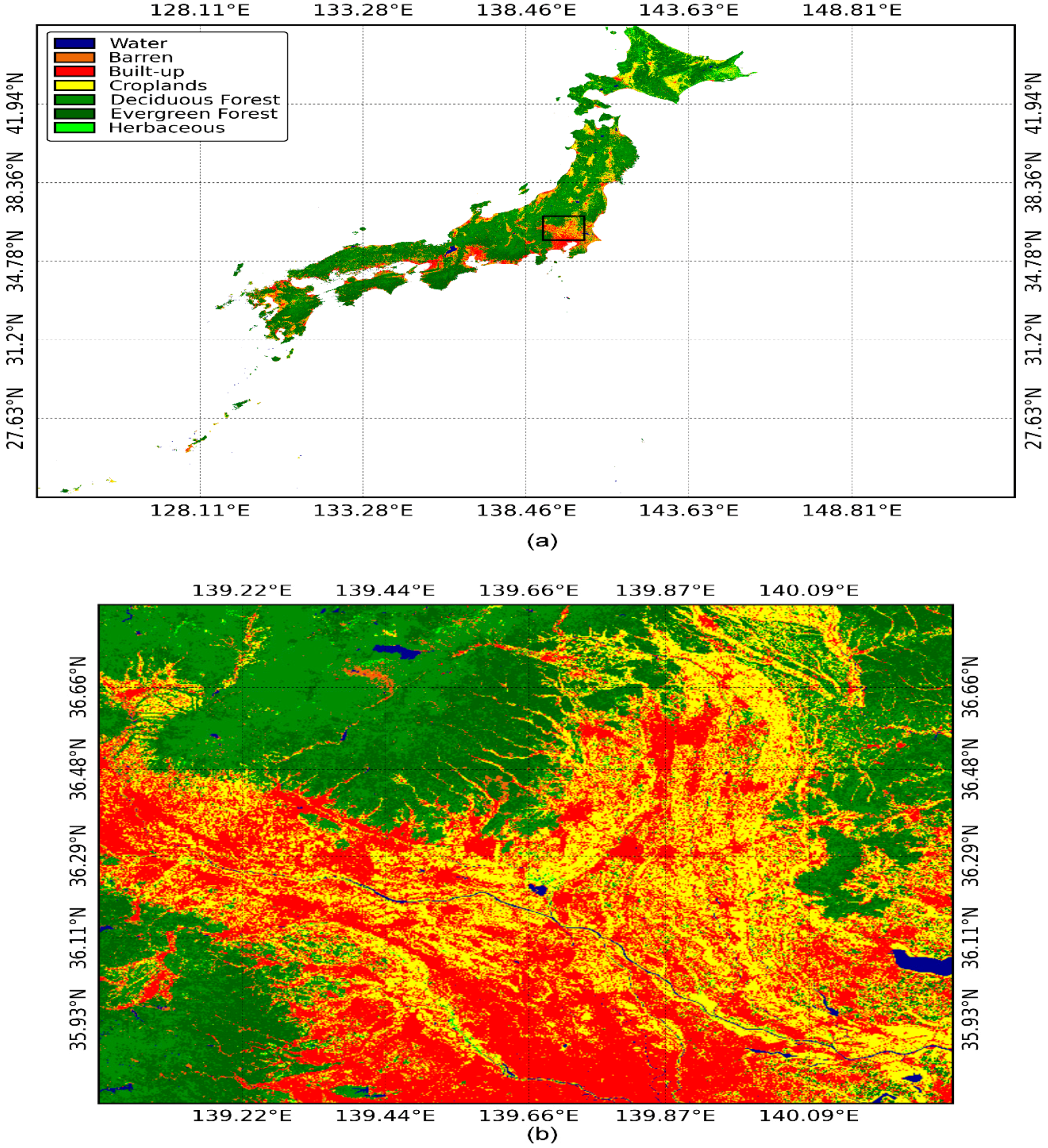
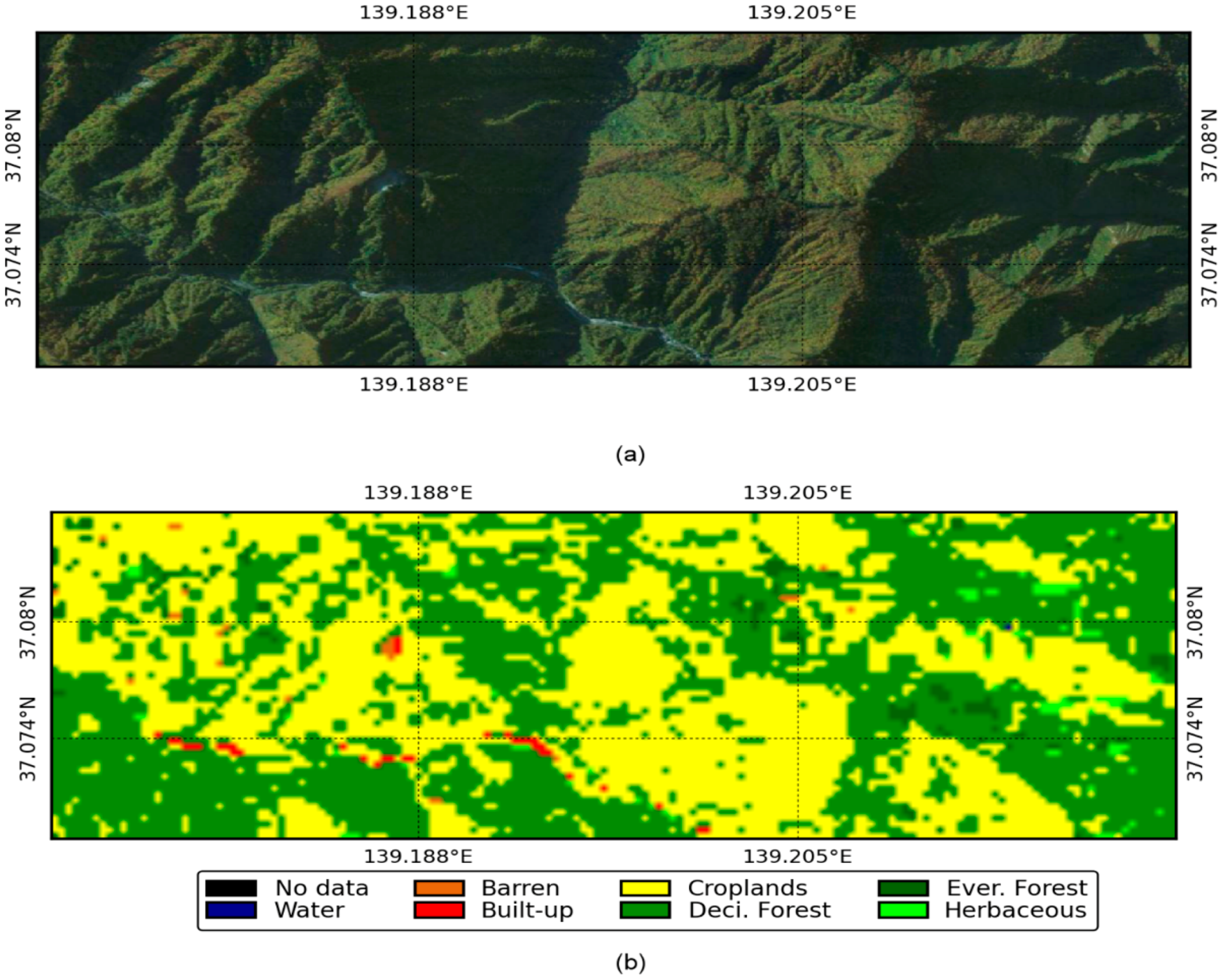
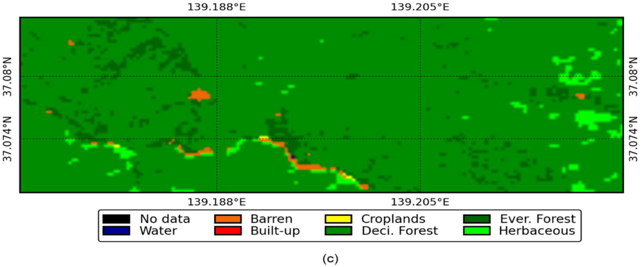
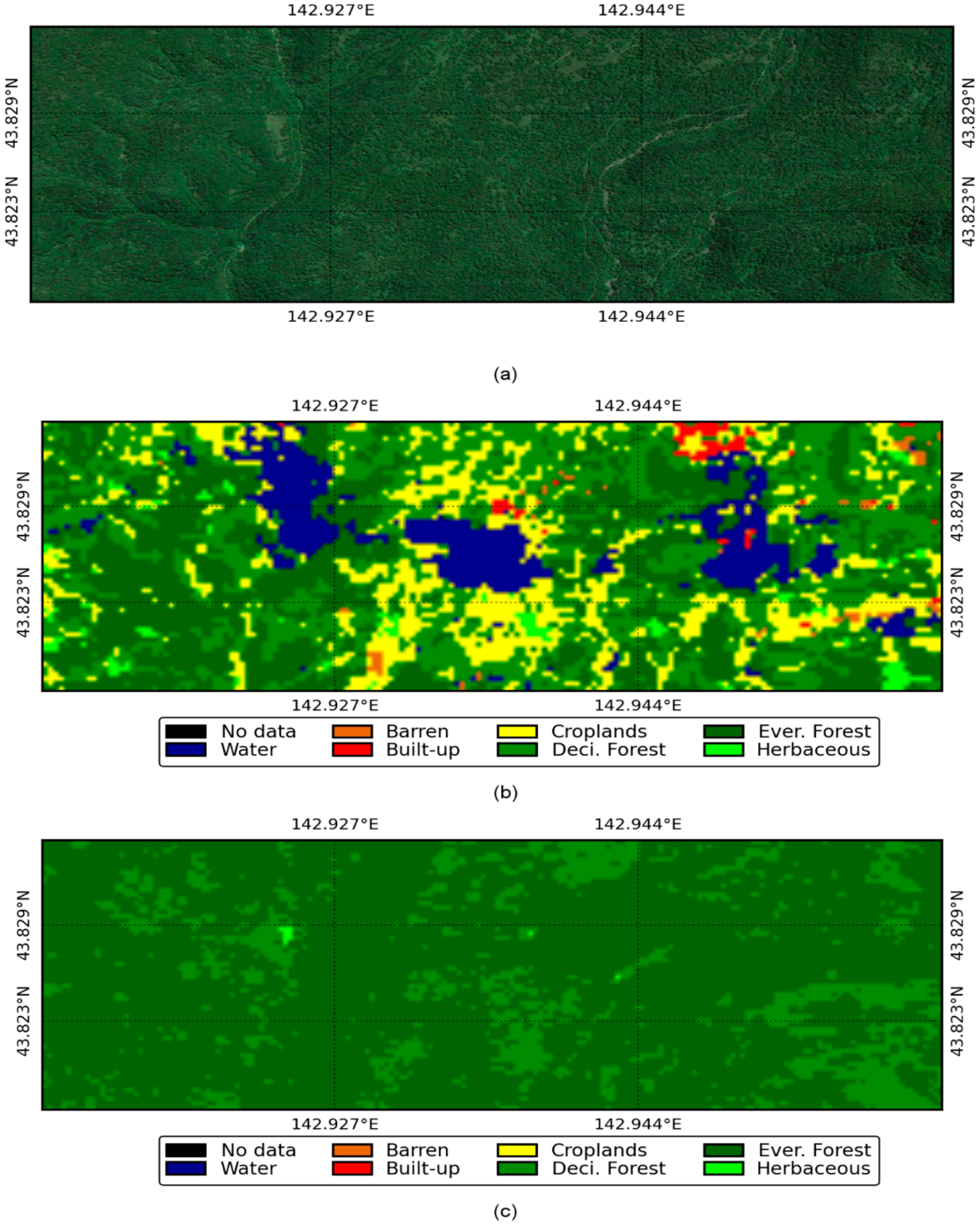
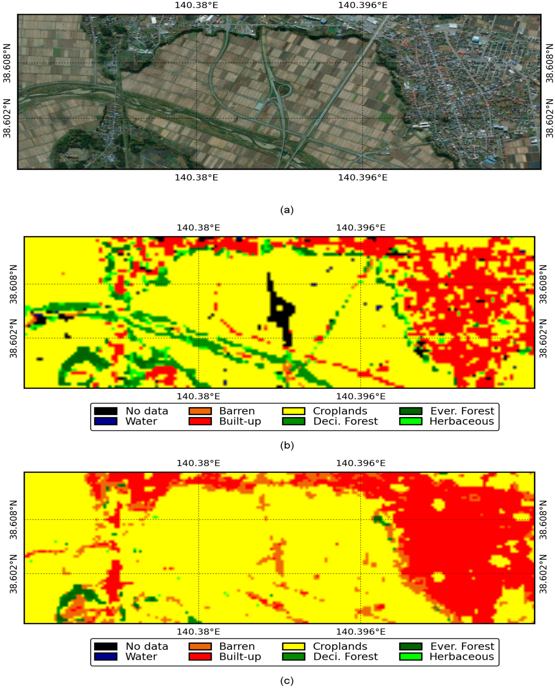
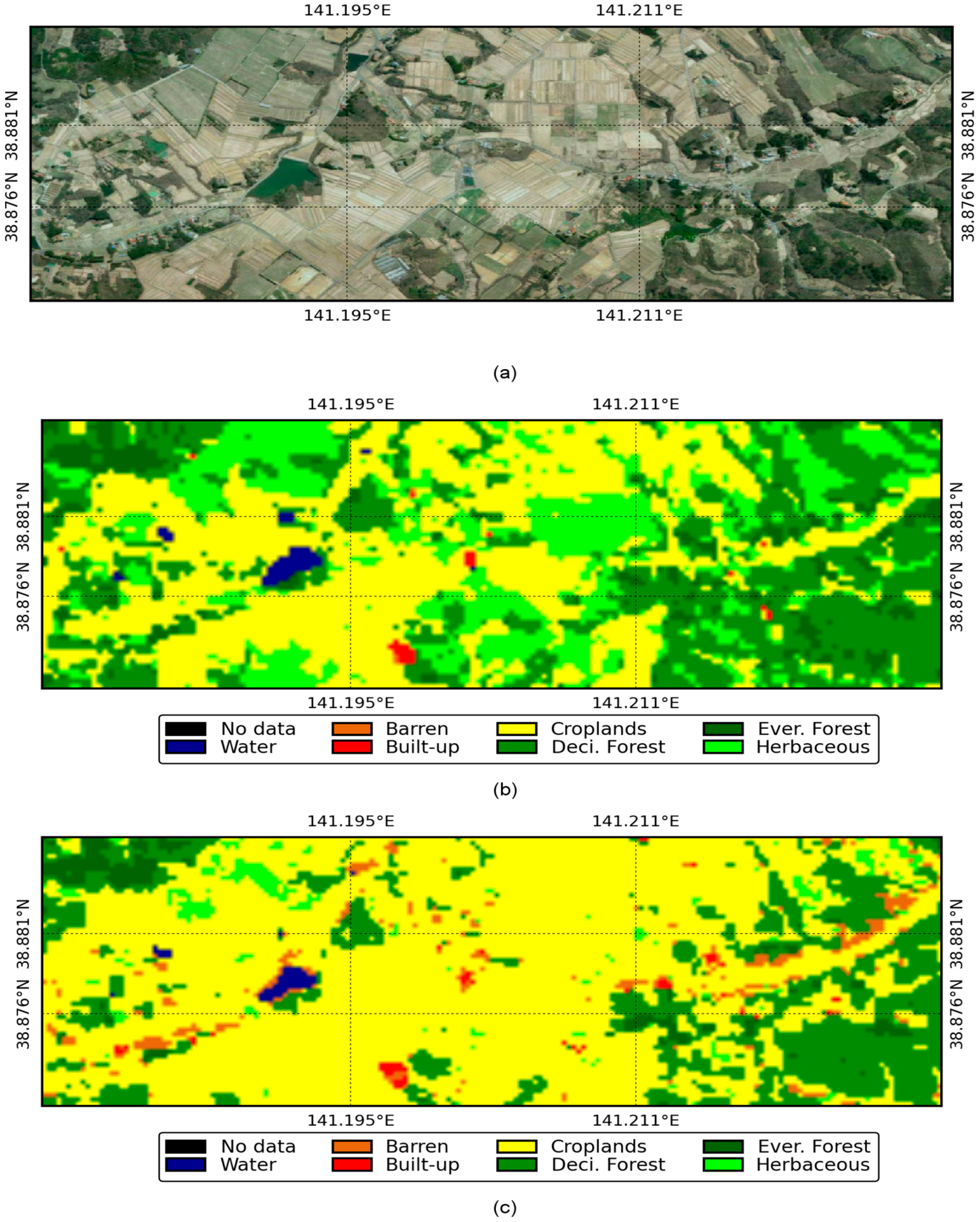
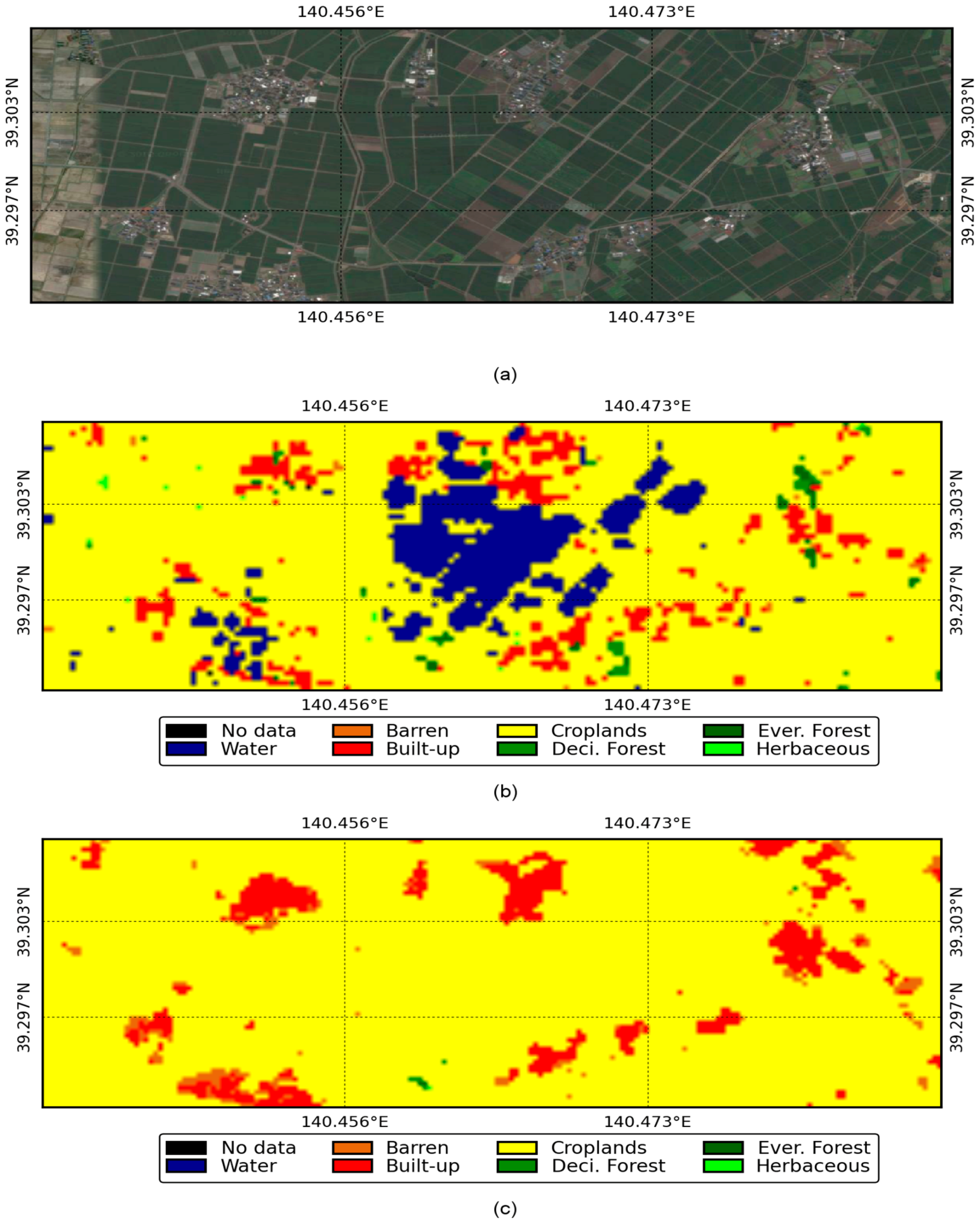
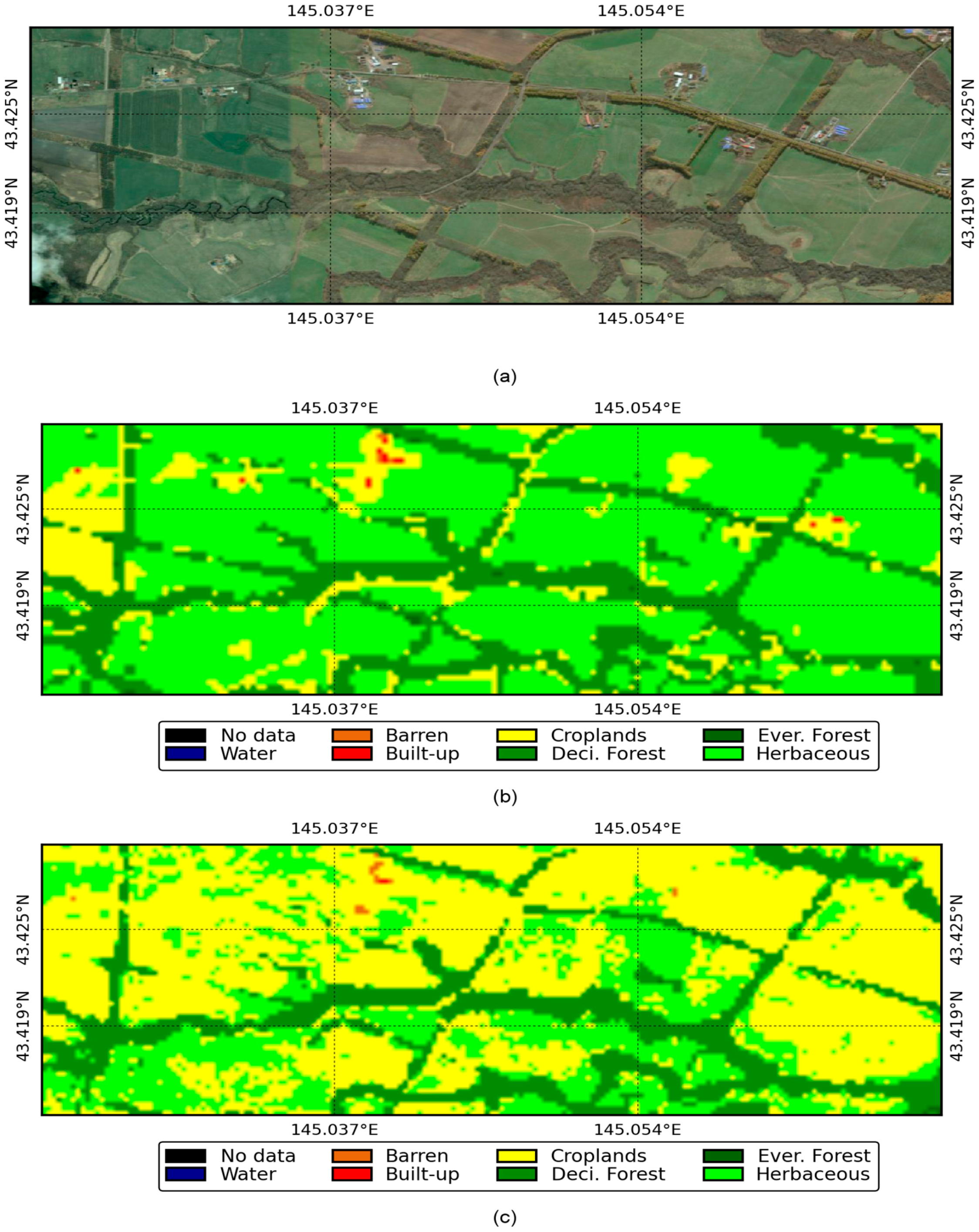
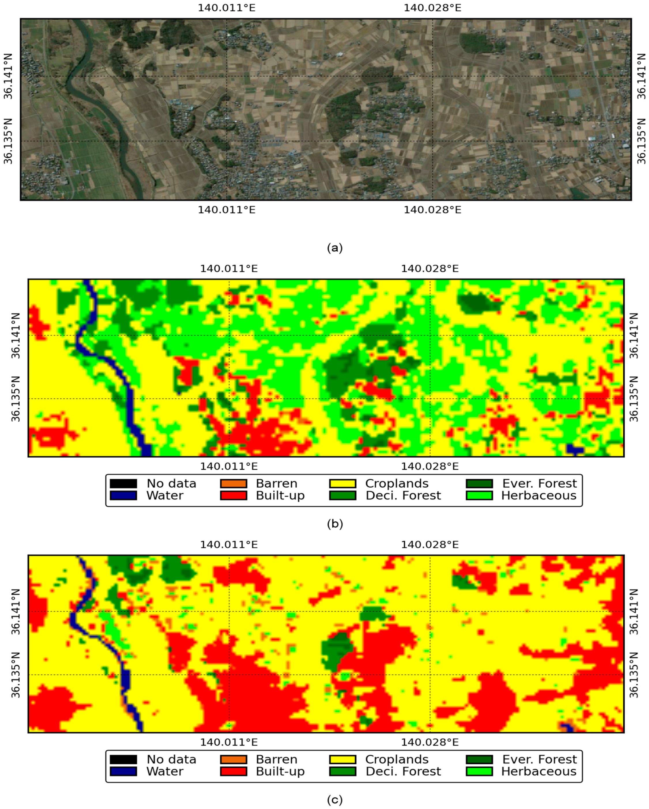
3.2. Production of the JpLC-30 Map

The 30-m resolution land cover map of Japan (JpLC-30 map) of 2013–2015 was produced based on the 45 optimum features selected. The resulting JpLC-30 map is shown in Figure 5.

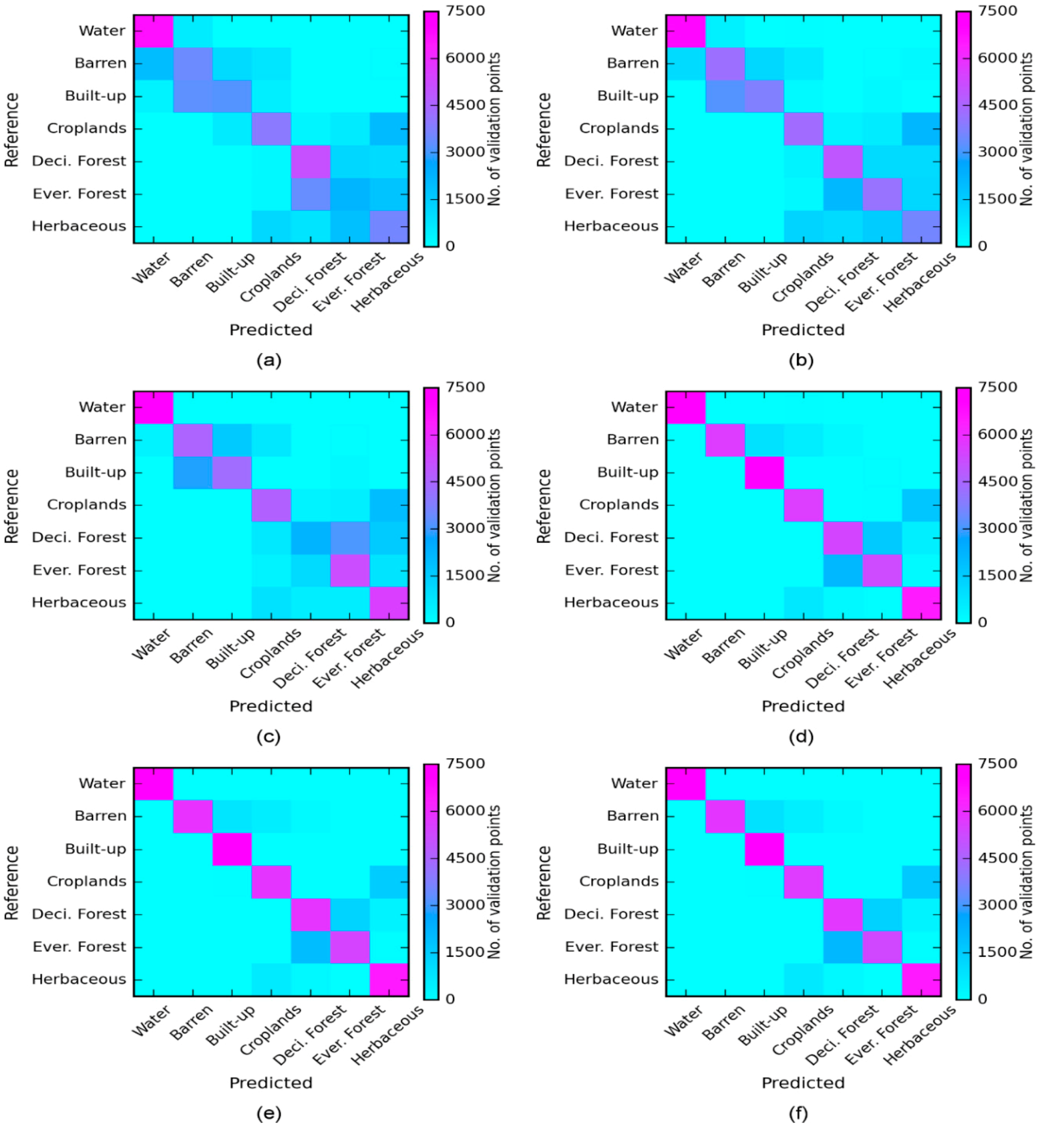
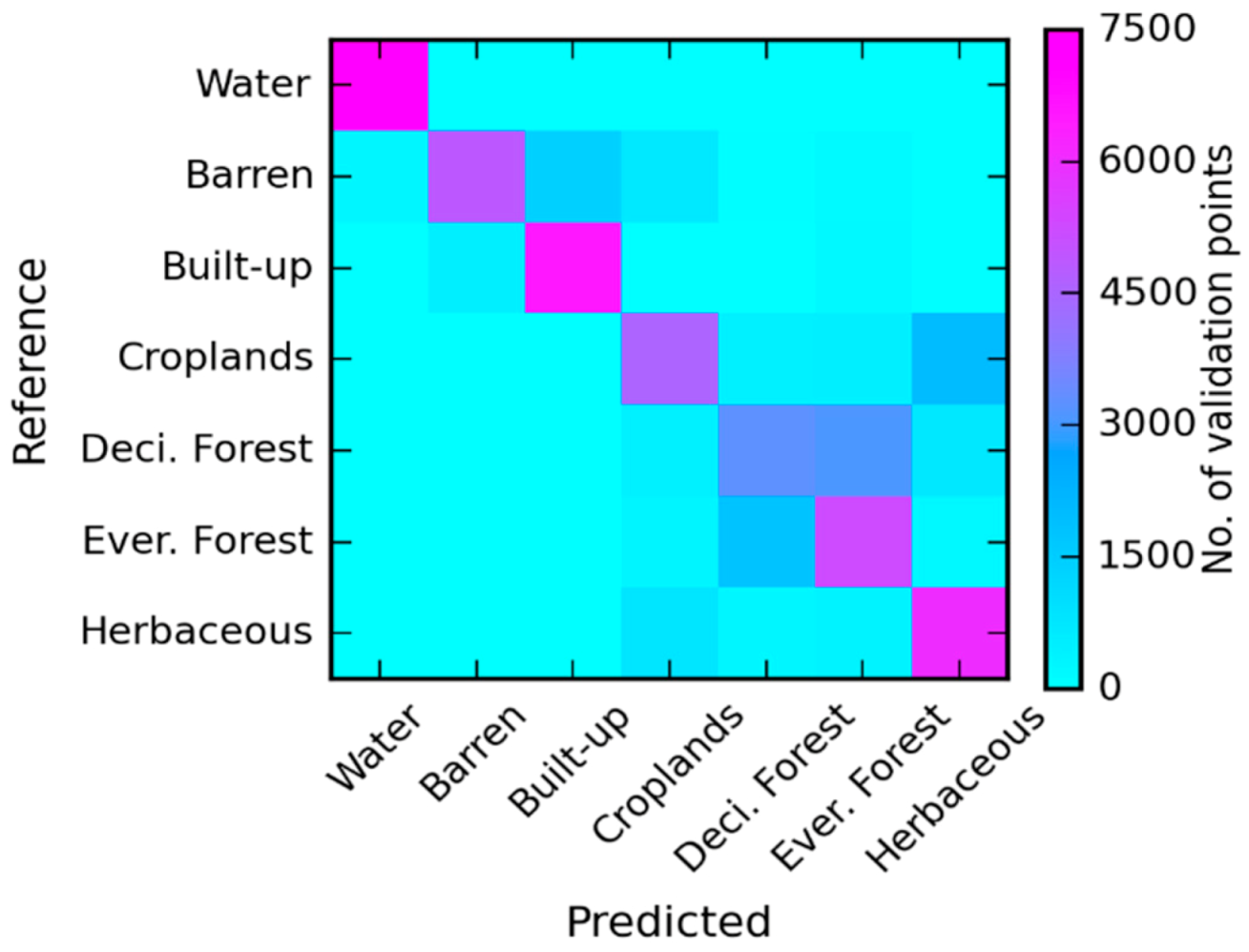
3.3. Performance Analysis

The resulting JpLC-30 map was compared to the existing JAXA High Resolution Land-Use and Land-Cover (JHR LULC Ver. 14.02) map of 2006–2011 with reference to the validation data collected in the research. The accuracy comparison between two maps was performed in a statistically-rigorous manner using the kappa coefficient [58], which measures inter-rater agreement for categorical variables by counting the proportion of instances that predictions agreed with the validation data (observed accuracy), after adjusting for the proportion of agreements taking place by chance (expected accuracy), as defined in Equation (1).

$$\text{Kappa}= \frac{\text{Observed accuracy}-\text{Expected accuracy}}{1-\text{Expected accuracy}}$$

(1)

Altogether 7500 validation points for each class distributed over the study area were used in the computation of the kappa coefficient. The validation data were the true ground location points visually verified with the Google Earth™ images and Landsat 8-based seasonal RGB images. Kappa coefficients calculated for the JpLC-30 and JHR LULC maps were 0.84 and 0.69, respectively. Based on the kappa coefficients, the JpLC-30 map is superior to the JHR LULC map. It should be noted that this analysis is solely based on validation points, which were not used for training the model for the production of the JpLC-30 map. The kappa coefficient was chosen over other accuracy metrics because it has been frequently used for assessing the accuracy of land cover maps.

The real-world performance of the JpLC-30 map was also evaluated in a number of places with reference to the Google Earth™ images of 2013–2015. The existing JHR LULC map was also used for comparison. For example, Figure 6, Figure 7, Figure 8, Figure 9, Figure 10, Figure 11, Figure 12, Figure 13, Figure 14, Figure 15 and Figure 16 demonstrate the performance of the JpLC-30 map over the existing map with reference to the Google Earth™ image. The JpLC-30 map has far better represented the land cover information than the JHR LULC map. Since the difference between the two maps is also derived from the annual change of the land cover itself, only a broad-scale discrepancy between the two maps in areas that are unlikely to fluctuate from the land cover changes, for example the occurrence of large water bodies over natural forests, was taken into consideration. As described in Figure 6, Figure 7, Figure 8, Figure 9, Figure 10, Figure 11, Figure 12, Figure 13, Figure 14, Figure 15 and Figure 16, the JHR LULC map has numerous classification errors pertinent to all land cover types. Major classification errors noticed in the JHR LULC map are: croplands in forests (Figure 6), water bodies in forests (Figure 7), water in croplands (Figure 8, Figure 9 and Figure 14) and herbaceous in croplands (Figure 13, Figure 15 and Figure 16). Moreover, the JHR LULC map has numerous unclassified/missing pixels (cf. the black pixels in Figure 10, Figure 11 and Figure 12), not only in volcanic mountains, but also in forests, croplands and urban built-up areas.

The random forests is a non-linear classifier. It consists of a large number of deep trees, where each tree is trained on the bagged data using the random selection of features, so gaining a full understanding of how the features interact non-linearly by examining each individual tree is infeasible. Therefore, to provide insights into how features interact linearly, the optimum features were further examined by using the Linear Discriminant Analysis (LDA; [59,60]). The LDA is the most commonly-used supervised image classification technique, which projects a feature space onto a smaller subspace and computes the linear discriminants that will maximize the separation between the multiple classes. The LDA-based confusion matrix as computed with the validation data yielded 69% overall accuracy (Figure 17). Hence, the linear classifier alone was able to provide more than two-thirds of the discrimination accuracy. Nevertheless, using the same features and validation data, the non-linear random forests classifier accelerated a recordable overall accuracy of up to 88.62% (Figure 4e).

The optimum features as selected from the random forests-based confusion matrix analysis are composed of the spectral, textural and topographic features of the land surface. Therefore, in a nutshell, the optimum features represent the bio-geo-physical phenomenon of the land surface. Different features are important in discriminating different land cover types pertaining to spatial-temporal dynamics. The random forests can handle highly non-linear interactions and classification boundaries of the bio-geo-physical features represented by the satellite data. The random forests classifier grows trees by searching random subspaces of the given data (features); the individual trees may change if the data are slightly changed, but the forest is relatively stable because it consists of many “random” trees. Therefore, the optimum set of features is unique to the given data, and the same set of optimum features may not be applied to other data, even for the same geographical location. Unlike theoretical models, supervised learning models are sensitive to features and the training data used for learning the model, because they analyze the training data and produce an optimum function to predict the class labels for unseen data by generalizing the training data. Due to the data-specific nature of the set of optimum features retrieved, they are not presented in the paper. However, models are to be learned with the new dataset before predicting results, and the optimum features can be chosen as described in this research. The selection of the optimum features is necessary to improve the prediction results and to boost the computing performance on very high-dimensional datasets.

Out of 45 feature images selected for optimum classification of land cover types, 43 features belonged to Landsat 8 spectral data; one feature belonged to the surface slope; and one feature belonged to the textural group (sum average). The sum average is the sum product of all neighboring pixels of a window (e.g., 3 × 3 pixels) used. The addition of textural information to the spectral signatures has been described as a valuable method for improving the land cover classification accuracy [61]. The best feature obtained in this research belonged to the textural group (sum average). It alone could yield 46.11% overall accuracy (Figure 4a). Out of 43 spectral features, all seven percentile values of NDVI were selected. This implies the importance of NDVI temporal information for discriminating land cover types.

The significant errors found in the JHR LULC map were the misclassification of urban areas and water bodies with forests and the misclassification of croplands with water bodies. The presence of deep shadows and the variety of the phenological spectra of the forests can misclassify urban built-up areas and water bodies mainly when limited temporal spectra are used for classification. Similarly, when croplands are classified by using water-fed period images only, paddy fields can be misclassified as water bodies. The misclassification errors present in the JHR LULC map may have resulted from limited temporal information carried out by the multi-spectral data and an insufficient number of training data used. The innovative data processing and mapping techniques used in the research have resulted in a highly accurate and seamless land cover map with the absence of unclassified/missing data pixels.

The higher accuracy achieved in the research suggests that the lower accuracy as reported by the existing automated mapping research (e.g., [45]) could be due to the insufficient representation of the temporal information by the sole utilization of green-season images. An effective utilization of multi-spectral, multi-textural and topographic features, as deployed in this research, is suggested for the production of a highly accurate land cover map. Nevertheless, the confusion matrix-based analysis (Figure 4e) with the validation data has indicated two major bottlenecks of the JpLC-30 map: misclassification between urban built-up areas and barren lands and misclassification between croplands and herbaceous. Due to similar spectral characteristics of urban built-up areas and barren lands, nighttime light data (500–1000-m resolution) are used for discriminating urban built-up areas from barren lands. However, the unavailability of higher resolution nighttime light data limits its applicability for 30-m resolution land cover mapping. Furthermore, the utilization of atmospherically-corrected reflectance data would be more accurate for large-scale mapping. The addition of higher resolution radar data-based (e.g., Sentinel 1A) multi-polarization and multi-textural features is expected to further increase the accuracy of the resultant JpLC-30 map.

4. Conclusions

Higher resolution (~30–50 m) land cover mapping at a large scale is complicated with the traditional manual processing, analysis and interpretation of huge volumes of data. Developing a technique that can automate the overall mapping procedures as much as possible is an inevitable solution for timely and reliable production of a higher resolution land cover map. The existing higher resolution land cover maps produced at national, regional and global scales have involved labor-intensive and time-consuming procedures. This research presented an automated technique for 30-m resolution land cover mapping at a national scale with high accuracy. The major attributes of the automated technique are the construction of a reference library by combining multi-spectral, multi-textural and topographic features and mapping by selecting the optimum number of features required for discriminating the land cover types. The reference library-driven feature-rich automated technique was used to produce the Japan 30-m resolution land cover (JpLC-30) map of 2013–2015. A comparative analysis of the JpLC-30 map with the existing 50-m resolution land cover map available in Japan (JHR LULC map) provided the superiority of the JpLC-30 map. The outcomes of this research highlight the feasibility of automated and repeat monitoring of land cover at the national, regional and even the global scale by the construction of a suitable reference library.

References

1. Vitousek, P.M.; Mooney, H.A.; Lubchenco, J.; Melillo, J.M. Human domination of earth’s ecosystems. Science 1997, 277, 494–499. [Google Scholar] [CrossRef]
2. Houghton, R.A.; Hackler, J.L.; Lawrence, K.T. The U.S. carbon budget: Contributions from land-use change. Science 1999, 285, 574–578. [Google Scholar] [CrossRef] [PubMed]
3. Foley, J.A.; DeFries, R.; Asner, G.P.; Barford, C.; Bonan, G.; Carpenter, S.R.; Chapin, F.S.; Coe, M.T.; Daily, G.C.; Gibbs, H.K. Global consequences of land use. Science 2005, 309, 570–574. [Google Scholar] [CrossRef] [PubMed]
4. Turner, B.L.; Lambin, E.F.; Reenberg, A. The emergence of land change science for global environmental change and sustainability. Proc. Natl. Acad. Sci. USA 2007, 104, 20666–20671. [Google Scholar] [CrossRef] [PubMed]
5. DeFries, R. Terrestrial vegetation in the coupled human-earth system: Contributions of remote sensing. Annu. Rev. Environ. Resour. 2008, 33, 369–390. [Google Scholar] [CrossRef]
6. Heald, C.L.; Spracklen, D.V. Land use change impacts on air quality and climate. Chem. Rev. 2015, 115, 4476–4496. [Google Scholar] [CrossRef] [PubMed]
7. Senapathi, D.; Carvalheiro, L.G.; Biesmeijer, J.C.; Dodson, C.-A.; Evans, R.L.; McKerchar, M.; Morton, R.D.; Moss, E.D.; Roberts, S.P.M.; Kunin, W.E. The impact of over 80 years of land cover changes on bee and wasp pollinator communities in England. Proc. R. Soc. Lond. B Biol. Sci. 2015, 282, 20150294. [Google Scholar] [CrossRef] [PubMed]
8. Bounoua, L.; DeFries, R.; Collatz, G.J.; Sellers, P.; Khan, H. Effects of land cover conversion on surface climate. Clim. Chang. 2002, 52, 29–64. [Google Scholar] [CrossRef]
9. Ge, J.; Qi, J.; Lofgren, B.M.; Moore, N.; Torbick, N.; Olson, J.M. Impacts of land use/cover classification accuracy on regional climate simulations. J. Geophys. Res. Atmos. 2007, 112. [Google Scholar] [CrossRef]
10. Hibbard, K.; Janetos, A.; van Vuuren, D.P.; Pongratz, J.; Rose, S.K.; Betts, R.; Herold, M.; Feddema, J.J. Research priorities in land use and land-cover change for the earth system and integrated assessment modelling. Int. J. Climatol. 2010, 30, 2118–2128. [Google Scholar] [CrossRef]
11. Ganzeveld, L.; Bouwman, L.; Stehfest, E.; van Vuuren, D.P.; Eickhout, B.; Lelieveld, J. Impact of future land use and land cover changes on atmospheric chemistry-climate interactions. J. Geophys. Res. Atmos. 2010, 115. [Google Scholar] [CrossRef]
12. DeFries, R.S.; Houghton, R.A.; Hansen, M.C.; Field, C.B.; Skole, D.; Townshend, J. Carbon emissions from tropical deforestation and regrowth based on satellite observations for the 1980s and 1990s. Proc. Natl. Acad. Sci. USA 2002, 99, 14256–14261. [Google Scholar] [CrossRef] [PubMed]
13. Jung, M.; Henkel, K.; Herold, M.; Churkina, G. Exploiting synergies of global land cover products for carbon cycle modeling. Remote Sens. Environ. 2006, 101, 534–553. [Google Scholar] [CrossRef]
14. Liu, J.; Vogelmann, J.E.; Zhu, Z.; Key, C.H.; Sleeter, B.M.; Price, D.T.; Chen, J.M.; Cochrane, M.A.; Eidenshink, J.C.; Howard, S.M. Estimating California ecosystem carbon change using process model and land cover disturbance data: 1951–2000. Ecol. Model. 2011, 222, 2333–2341. [Google Scholar] [CrossRef]
15. Poulter, B.; Frank, D.C.; Hodson, E.L.; Zimmermann, N.E. Impacts of land cover and climate data selection on understanding terrestrial carbon dynamics and the CO2 airborne fraction. Biogeosciences 2011, 8, 2027–2036. [Google Scholar] [CrossRef]
16. Buchanan, G.M.; Nelson, A.; Mayaux, P.; Hartley, A.; Donald, P.F. Delivering a global, terrestrial, biodiversity observation system through remote sensing. Conserv. Biol. 2009, 23, 499–502. [Google Scholar] [CrossRef] [PubMed]
17. De Baan, L.; Curran, M.; Rondinini, C.; Visconti, P.; Hellweg, S.; Koellner, T. High-resolution assessment of land use impacts on biodiversity in life cycle assessment using species habitat suitability models. Environ. Sci. Technol. 2015, 49, 2237–2244. [Google Scholar] [CrossRef] [PubMed]
18. Liang, L.; Xu, B.; Chen, Y.; Liu, Y.; Cao, W.; Fang, L.; Feng, L.; Goodchild, M.F.; Gong, P.; Li, W. Combining spatial-temporal and phylogenetic analysis approaches for improved understanding on global H5N1 transmission. PLoS ONE 2010, 5, e13575. [Google Scholar] [CrossRef] [PubMed] [Green Version]
19. Foody, G.M. Status of land cover classification accuracy assessment. Remote Sens. Environ. 2002, 80, 185–201. [Google Scholar] [CrossRef]
20. Friedl, M.A.; Sulla-Menashe, D.; Tan, B.; Schneider, A.; Ramankutty, N.; Sibley, A.; Huang, X. MODIS Collection 5 global land cover: Algorithm refinements and characterization of new datasets. Remote Sens. Environ. 2010, 114, 168–182. [Google Scholar] [CrossRef]
21. Tateishi, R.; Hoan, N.T.; Kobayashi, T.; Alsaaideh, B.; Tana, G.; Phong, D.X. Production of global land cover data–GLCNMO2008. J. Geogr. Geol. 2014, 6, 99–122. [Google Scholar] [CrossRef]
22. Thenkabail, P.S.; Biradar, C.M.; Noojipady, P.; Dheeravath, V.; Li, Y.; Velpuri, M.; Gumma, M.; Gangalakunta, O.R.P.; Turral, H.; Cai, X.; et al. Global irrigated area map (GIAM), derived from remote sensing, for the end of the last millennium. Int. J. Remote Sens. 2009, 30, 3679–3733. [Google Scholar] [CrossRef]
23. Salmon, J.M.; Friedl, M.A.; Frolking, S.; Wisser, D.; Douglas, E.M. Global rain-fed, irrigated, and paddy croplands: A new high resolution map derived from remote sensing, crop inventories and climate data. Int. J. Appl. Earth Observ. Geoinform. 2015, 38, 321–334. [Google Scholar] [CrossRef]
24. Feng, M.; Sexton, J.O.; Channan, S.; Townshend, J.R. A global, high-resolution (30-m) inland water body dataset for 2000: First results of a topographic–spectral classification algorithm. Int. J. Dig. Earth 2015, 9, 1–21. [Google Scholar] [CrossRef]
25. Sharma, R.C.; Tateishi, R.; Hara, K.; Nguyen, L.V. Developing superfine water index (SWI) for global water cover mapping using MODIS data. Remote Sens. 2015, 7, 13807–13841. [Google Scholar] [CrossRef]
26. Ban, Y.; Jacob, A.; Gamba, P. Spaceborne SAR data for global urban mapping at 30m resolution using a robust urban extractor. ISPRS J. Photogramm. Remote Sens. 2015, 103, 28–37. [Google Scholar] [CrossRef]
27. Zhou, Y.; Smith, S.J.; Zhao, K.; Imhoff, M.; Thomson, A.; Bond-Lamberty, B.; Asrar, G.R.; Zhang, X.; He, C.; Elvidge, C.D. A global map of urban extent from nightlights. Environ. Res. Lett. 2015, 10, 054011. [Google Scholar] [CrossRef]
28. Fluet-Chouinard, E.; Lehner, B.; Rebelo, L.-M.; Papa, F.; Hamilton, S.K. Development of a global inundation map at high spatial resolution from topographic downscaling of coarse-scale remote sensing data. Remote Sens. Environ. 2015, 158, 348–361. [Google Scholar] [CrossRef]
29. Hansen, M.C.; Potapov, P.V.; Moore, R.; Hancher, M.; Turubanova, S.A.; Tyukavina, A.; Thau, D.; Stehman, S.V.; Goetz, S.J.; Loveland, T.R. High-resolution global maps of 21st-century forest cover change. Science 2013, 342, 850–853. [Google Scholar] [CrossRef] [PubMed]
30. Shimada, M.; Itoh, T.; Motooka, T.; Watanabe, M.; Shiraishi, T.; Thapa, R.; Lucas, R. New global forest/non-forest maps from ALOS PALSAR data (2007–2010). Remote Sens. Environ. 2014, 155, 13–31. [Google Scholar] [CrossRef]
31. Herold, M.; Mayaux, P.; Woodcock, C.E.; Baccini, A.; Schmullius, C. Some challenges in global land cover mapping: An assessment of agreement and accuracy in existing 1 km datasets. Remote Sens. Environ. 2008, 112, 2538–2556. [Google Scholar] [CrossRef]
32. McCallum, I.; Obersteiner, M.; Nilsson, S.; Shvidenko, A. A spatial comparison of four satellite derived 1 km global land cover datasets. Int. J. Appl. Earth Observ. Geoinform. 2006, 8, 246–255. [Google Scholar] [CrossRef]
33. Congalton, R.; Gu, J.; Yadav, K.; Thenkabail, P.; Ozdogan, M. Global land cover mapping: A review and uncertainty analysis. Remote Sens. 2014, 6, 12070–12093. [Google Scholar] [CrossRef]
34. Yu, L.; Liang, L.; Wang, J.; Zhao, Y.; Cheng, Q.; Hu, L.; Liu, S.; Yu, L.; Wang, X.; Zhu, P. Meta-discoveries from a synthesis of satellite-based land-cover mapping research. Int. J. Remote Sens. 2014, 35, 4573–4588. [Google Scholar] [CrossRef]
35. Grekousis, G.; Mountrakis, G.; Kavouras, M. An overview of 21 global and 43 regional land-cover mapping products. Int. J. Remote Sens. 2015, 36, 5309–5335. [Google Scholar] [CrossRef]
36. Giri, C.; Pengra, B.; Long, J.; Loveland, T.R. Next generation of global land cover characterization, mapping, and monitoring. Int. J. Appl. Earth Observ. Geoinform. 2013, 25, 30–37. [Google Scholar] [CrossRef]
37. Homer, C.; Huang, C.; Yang, L.; Wylie, B.; Coan, M. Development of a 2001 national land-cover database for the United States. Photogramm. Eng. Remote Sens. 2004, 70, 829–840. [Google Scholar] [CrossRef]
38. Homer, C.; Dewitz, J.; Fry, J.; Coan, M.; Hossain, N.; Larson, C.; Herold, N.; McKerrow, A.; VanDriel, J.N.; Wickham, J. Completion of the 2001 national land cover database for the counterminous United States. Photogramm. Eng. Remote Sens. 2007, 73, 337–341. [Google Scholar]
39. Homer, C.; Dewitz, J.; Yang, L.; Jin, S.; Danielson, P.; Xian, G.; Coulston, J.; Herold, N.; Wickham, J.; Megown, K. Completion of the 2011 national land cover database for the conterminous United States–Representing a decade of land cover change information. Photogramm. Eng. Remote Sens. 2015, 81, 345–354. [Google Scholar]
40. Chen, J.; Chen, J.; Liao, A.; Cao, X.; Chen, L.; Chen, X.; He, C.; Han, G.; Peng, S.; Lu, M. Global land cover mapping at 30 m resolution: A POK-based operational approach. ISPRS J. Photogramm. Remote Sens. 2015, 103, 7–27. [Google Scholar] [CrossRef]
41. Giri, C.; Long, J. Land cover characterization and mapping of South America for the year 2010 using Landsat 30 m satellite data. Remote Sens. 2014, 6, 9494–9510. [Google Scholar] [CrossRef]
42. Takahashi, M.; Nasahara, K.N.; Tadono, T.; Watanabe, T.; Dotsu, M.; Sugimura, T.; Tomiyama, N. JAXA high resolution land-use and land-cover map of Japan. In Proceedings of the IEEE International Geoscience and Remote Sensing Symposium, Melbourne, Australia, 21–26 July 2013; pp. 2384–2387.
43. Himiyama, Y. Land use/cover changes in Japan: From the past to the future. Hydrol. Process. 1998, 12, 1995–2001. [Google Scholar] [CrossRef]
44. Harada, I.; Hara, K.; Tomita, M.; Short, K.; Park, J. Monitoring landscape changes in Japan using classification of MODIS data combined with a landscape transformation sere (LTS) model. J. Landsc. Ecol. 2015, 7, 23–28. [Google Scholar] [CrossRef]
45. Gong, P.; Wang, J.; Yu, L.; Zhao, Y.; Zhao, Y.; Liang, L.; Niu, Z.; Huang, X.; Fu, H.; Liu, S. Finer resolution observation and monitoring of global land cover: First mapping results with Landsat TM and ETM+ data. Int. J. Remote Sens. 2013, 34, 2607–2654. [Google Scholar] [CrossRef]
46. Irons, J.R.; Dwyer, J.L.; Barsi, J.A. The next Landsat satellite: The Landsat Data Continuity Mission. Remote Sens. Environ. 2012, 122, 11–21. [Google Scholar] [CrossRef]
47. Roy, D.P.; Wulder, M.A.; Loveland, T.R.; Woodcock, C.E.; Allen, R.G.; Anderson, M.C.; Helder, D.; Irons, J.R.; Johnson, D.M.; Kennedy, R.; et al. Landsat-8: Science and product vision for terrestrial global change research. Remote Sens. Environ. 2014, 145, 154–172. [Google Scholar] [CrossRef]
48. Tucker, C.J. Red and photographic infrared linear combinations for monitoring vegetation. Remote Sens. Environ. 1979, 8, 127–150. [Google Scholar] [CrossRef]
49. Haralick, R.M.; Shanmugam, K.; Dinstein, I. Textural features for image classification. IEEE Trans. Syst. Man Cybern. 1973, SMC-3, 610–621. [Google Scholar] [CrossRef]
50. Conners, R.W.; Trivedi, M.M.; Harlow, C.A. Segmentation of a high-resolution urban scene using texture operators. Comput. Vis. Graph. Image Process. 1984, 25, 273–310. [Google Scholar] [CrossRef]
51. Bishop, C.M. Pattern Recognition and Machine Learning; Information Science and Statistics; Springer: New York, NY, USA, 2006. [Google Scholar]
52. Breiman, L.; Friedman, J.H.; Olshen, R.A.; Stone, C.J. Classification and Regression Trees; Wadsworth: Belmont, CA, USA, 1984. [Google Scholar]
53. Breiman, L. Random forests. Mach. Learn. 2001, 45, 5–32. [Google Scholar] [CrossRef]
54. Pal, M. Random forest classifier for remote sensing classification. Int. J. Remote Sens. 2005, 26, 217–222. [Google Scholar] [CrossRef]
55. Gislason, P.O.; Benediktsson, J.A.; Sveinsson, J.R. Random forests for land cover classification. Pattern Recognit. Lett. 2006, 27, 294–300. [Google Scholar] [CrossRef]
56. Rodriguez-Galiano, V.F.; Chica-Olmo, M.; Abarca-Hernandez, F.; Atkinson, P.M.; Jeganathan, C. Random forest classification of Mediterranean land cover using multi-seasonal imagery and multi-seasonal texture. Remote Sens. Environ. 2012, 121, 93–107. [Google Scholar] [CrossRef]
57. Hayes, M.M.; Miller, S.N.; Murphy, M.A. High-resolution landcover classification using Random Forest. Remote Sens. Lett. 2014, 5, 112–121. [Google Scholar] [CrossRef]
58. Cohen, J. A Coefficient of agreement for nominal scales. Educ. Psychol. Meas. 1960, 20, 37–46. [Google Scholar] [CrossRef]
59. Fisher, R.A. The use of multiple measurements in taxonomic problems. Ann. Eugen. 1936, 7, 179–188. [Google Scholar] [CrossRef]
60. Rao, C.R. The utilization of multiple measurements in problems of biological classification. J. R. Stat. Soc. Ser. B (Methodol.) 1948, 10, 159–203. [Google Scholar]
61. Lu, D.; Li, G.; Moran, E.; Dutra, L.; Batistella, M. The roles of textural images in improving land-cover classification in the Brazilian Amazon. Int. J. Remote Sens. 2014, 35, 8188–8207. [Google Scholar] [CrossRef]
Figure 1. The data processing steps involved in the preparation of feature images used in the research. The input datasets are shown in bold.
Remotesensing 08 00429 g001
Figure 2. The distribution of reference (training and validation) data: (a) display of the national territory; (b) zoomed in over the black polygon region in (a) showing the density of the reference points. The national boundary is based on the Global Administrative Areas database (GADM) Version 2.8, November 2015.
Remotesensing 08 00429 g002
Figure 3. Variation of the confusion matrix-based overall accuracy (%) with respect to the number of features used.
Remotesensing 08 00429 g003
Figure 4. The confusion matrix with different numbers of best features used: (a) overall accuracy = 46.11%, No. of features = 1; (b) overall accuracy = 50.57%, No. of features = 2; (c) overall accuracy = 66.92%, No. of features = 5; (d) overall accuracy = 85.55%, No. of features = 15; (e) overall accuracy = 88.62%, No. of features = 45; (f) overall accuracy = 88.58%, No. of features = 68.
Remotesensing 08 00429 g004
Figure 5. Japan 30-m land cover (JpLC-30) map of 2013–2015 produced through the research: (a) display of the national territory; (b) zoomed in over the black polygon region in (a). The national boundary is based on the Global Administrative Areas database (GADM) Version 2.8, November 2015.
Remotesensing 08 00429 g005
Figure 6. Performance of the JpLC-30 map over the JAXA High Resolution Land-Use and Land-Cover (JHR LULC) map: (a) Google Earth™ image; (b) JHR LULC map; (c) JpLC-30 map.
Remotesensing 08 00429 g006aRemotesensing 08 00429 g006b
Figure 7. Performance of the JpLC-30 map over the JHR LULC map: (a) Google Earth™ image; (b) JHR LULC map; (c) JpLC-30 map.
Remotesensing 08 00429 g007
Figure 8. Performance of the JpLC-30 map over the JHR LULC map: (a) Google Earth™ image; (b) JHR LULC map; (c) JpLC-30 map.
Remotesensing 08 00429 g008
Figure 9. Performance of the JpLC-30 map over the JHR LULC map: (a) Google Earth™ image; (b) JHR LULC map; (c) JpLC-30 map.
Remotesensing 08 00429 g009
Figure 10. Performance of the JpLC-30 map over the JHR LULC map: (a) Google Earth™ image; (b) JHR LULC map; (c) JpLC-30 map.
Remotesensing 08 00429 g010
Figure 11. Performance of the JpLC-30 map over the JHR LULC map: (a) Google Earth™ image; (b) JHR LULC map; (c) JpLC-30 map.
Remotesensing 08 00429 g011
Figure 12. Performance of the JpLC-30 map over the JHR LULC map: (a) Google Earth™ image; (b) JHR LULC map; (c) JpLC-30 map.
Remotesensing 08 00429 g012
Figure 13. Performance of the JpLC-30 map over the JHR LULC map: (a) Google Earth™ image; (b) JHR LULC map; (c) JpLC-30 map.
Remotesensing 08 00429 g013
Figure 14. Performance of the JpLC-30 map over the JHR LULC map: (a) Google Earth™ image; (b) JHR LULC map; (c) JpLC-30 map.
Remotesensing 08 00429 g014
Figure 15. Performance of the JpLC-30 map over the JHR LULC map: (a) Google Earth™ image; (b) JHR LULC map; (c) JpLC-30 map.
Remotesensing 08 00429 g015
Figure 16. Performance of the JpLC-30 map over the JHR LULC map: (a) Google Earth™ image; (b) JHR LULC map; (c) JpLC-30 map.
Remotesensing 08 00429 g016
Figure 17. Linear Discriminant Analysis (LDA)-based confusion matrix.
Remotesensing 08 00429 g017