1. Introduction
Orbiting around the Sun–Earth L1 Lagrange point, the two instruments on board the Deep Space Climate Observatory (DSCOVR) spacecraft, the Earth Polychromatic Imaging Camera (EPIC) and the National Institute of Standards and Technology Advanced Radiometer (NISTAR), provide observations on the entire sunlit side of the Earth continuously [
1]. Like any other satellite, DSCOVR can only discretely sample the Earth’s climate system. Factors such as the dowlink bandwidth and receiver antenna availability also affect the number of observations that can be sent back. As has been shown in previous studies, this subsampling will affect the accuracy of satellite retrieved parameters [
2,
3]. The potential effects of temporal sampling frequency on the Earth’s radiation budget derived from DSCOVR-like observations have been assessed using a range of different metrics in Part 1 of this study ([
4]—hereafter, Part-1). Another important product of DSCOVR-EPIC is the cloud fraction. This paper will address how temporal sampling frequency affects this quantity with a similar approach as Part-1.
EPIC observes the Earth with 10 spectral channels ranging from the ultraviolet to the near infrared with a 2048 by 2048 CCD array. At the vantage point of L1, EPIC provides snapshots of the cloud fields for the entire sunlit half of the Earth, which is valuable in interpreting the NISTAR observations and in climate applications. To study the effect of temporal sampling, a baseline truth dataset is needed. As in Part 1, the Goddard Earth Observing System version-5 (GEOS-5) Nature Run cloud fields are used as “truth”. The Nature Run is well-suited for this purpose because of its high spatial and temporal resolution. It is run with a 7 km horizontal resolution, 72 model levels up to 0.01 hPa and with a timestep of a few minutes. The Nature Run provides a two year time series of an atmospheric state that is dynamically consistent. As discussed in Part 1 and the references therein (e.g., [
5,
6,
7]), the GEOS-5 Nature Run and operational systems have been carefully validated against satellite data and shown to maintain a realistic atmospheric state throughout the length of integration.
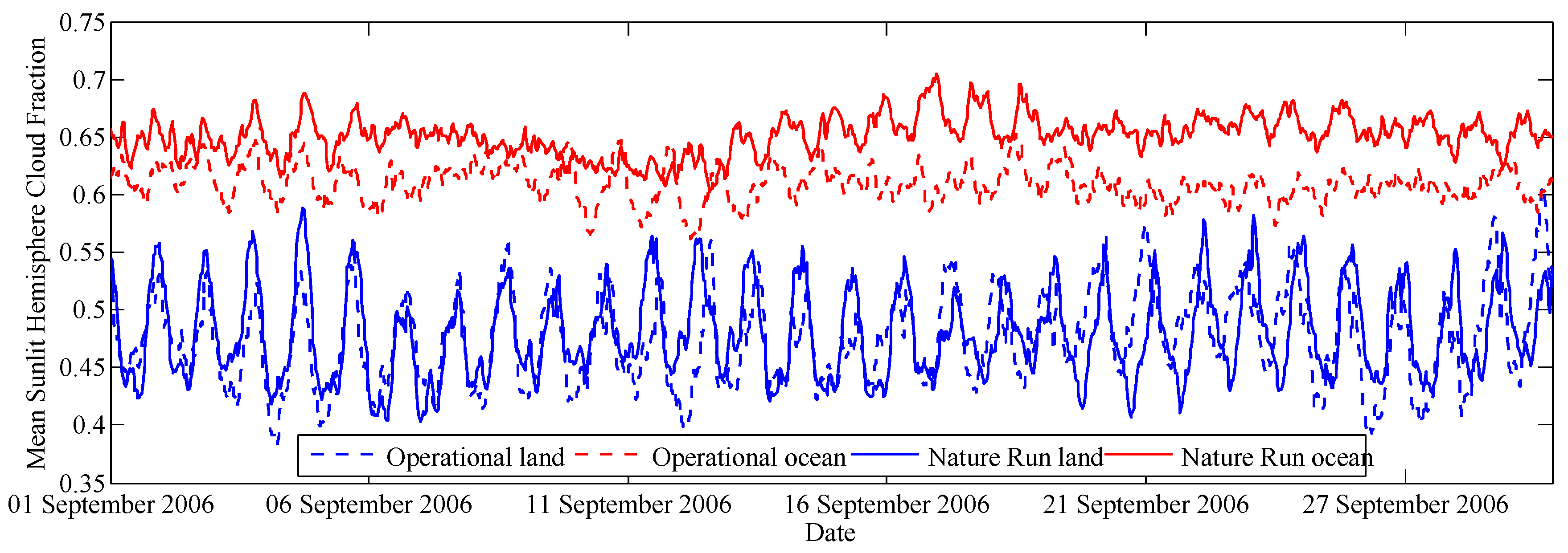
A comparison between the current GEOS-5 operational system and the Nature Run mean total cloud fraction for September 2006 is shown in
Figure 1. The maximum operational forecast length is 24 h. Although differences exist, as expected, the cloud fraction produced by the Nature Run has similar temporal variations to that seen in GEOS-5 operational products. For ocean cloud fraction, there is a slight positive bias for the Nature Run, but the variations and the land cloud fraction are very similar between the two models. Compared to the operational system, it is clear that the Nature Run field exhibits similar scales and structures. The Nature Run captures smaller-scale variations than the operational model due to the higher spatial and temporal resolution, which is beneficial in terms of testing the limits of temporal sampling frequency.
Figure 2 shows a snapshot of the cloud fraction for the sunlit side of the Earth from the Nature Run at 1200 UTC on 25 September 2006. The image shows the field from the perspective of EPIC. For every time step of the Nature Run, a cloud field similar to
Figure 2 can be generated. Analysis in this study is based on the mean cloud fraction of these simulated snapshots.
The paper is arranged as follows:
Section 2 recaps the methodology outlined in Part-1 and introduces any new methodology used here.
Section 3 shows all of the results for different sampling frequencies and discusses the implications for DSCOVR.
Section 4 provides the concluding remarks.
3. Results
The Nature Run provides cloud fractions at different altitudes: high , middle , low , and total . For each altitude region, high, middle, and low, the maximum column cloud fraction between an upper and lower height is taken. The total cloud fraction is given using a random overlapping assumption . The mean total cloud fraction is computed for the entire sunlit half of the Earth—the same area that EPIC observes. To take into account the differences between clouds over ocean and over land, cloud fraction for the two different surface types are considered separately.
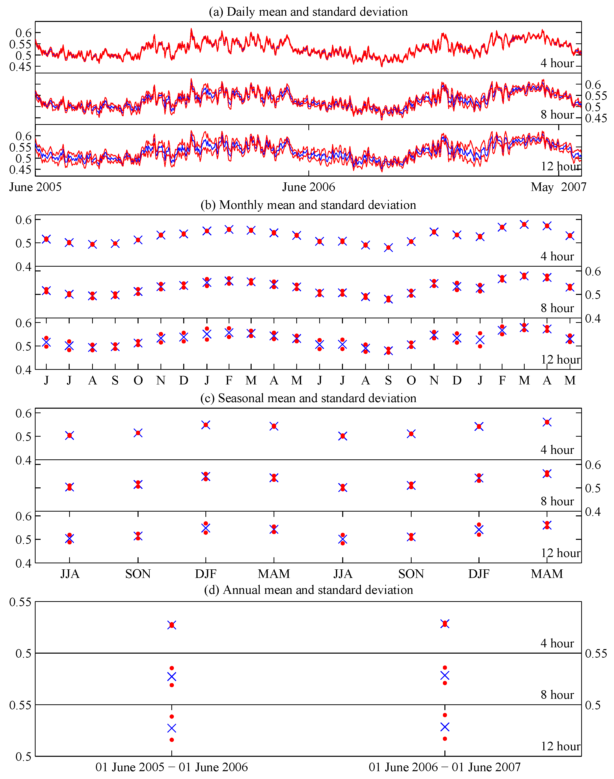
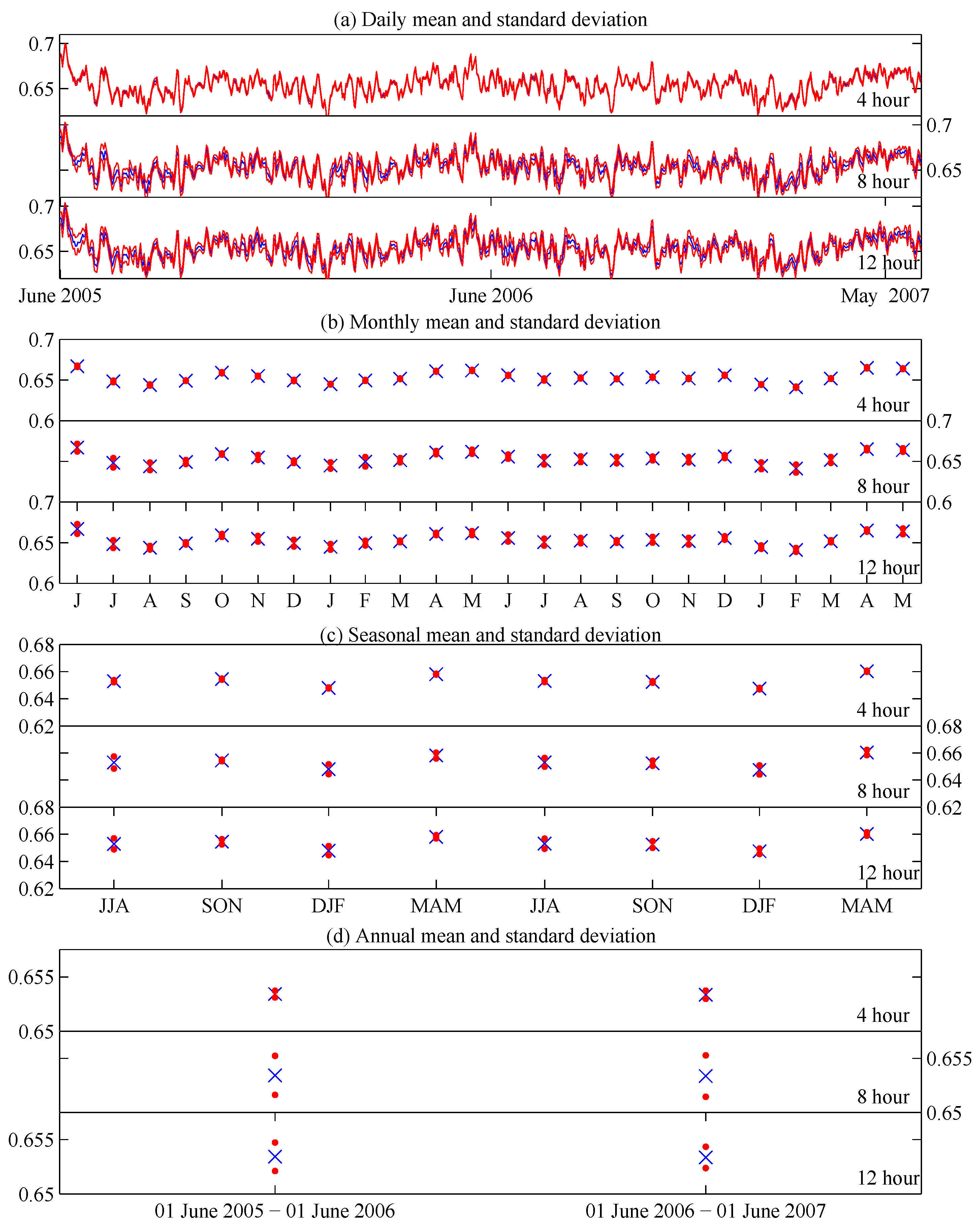
Figure 3a shows the daily mean
and mean plus and minus one standard deviation of the difference between full and subsampled time series
for the 720 days of the Nature Run. The figure shows the results for the total cloud fraction
over land. The three panels show the results for the
4-, 8-, and 12-h sampling frequency.
Figure 3b shows the monthly mean and standard deviation of the difference between full and subsampled time series;
Figure 3c shows the seasonal values; and
Figure 3d shows the annual values. Note that vertical scaling is kept fixed within each of the three sub-panels, but is not fixed for the entire figure.
Figure 3 shows that variations in the daily mean during the northern hemisphere winter season are greater than that during the summer months. At this time of year, a greater area of ocean is visible from the L1 Lagrange point as the large land masses of the northern hemisphere are orientated away from the sun. Due to the constantly changing character of cloud fields, the smaller the geographical area being included in the calculation, the larger the variation that is expected.
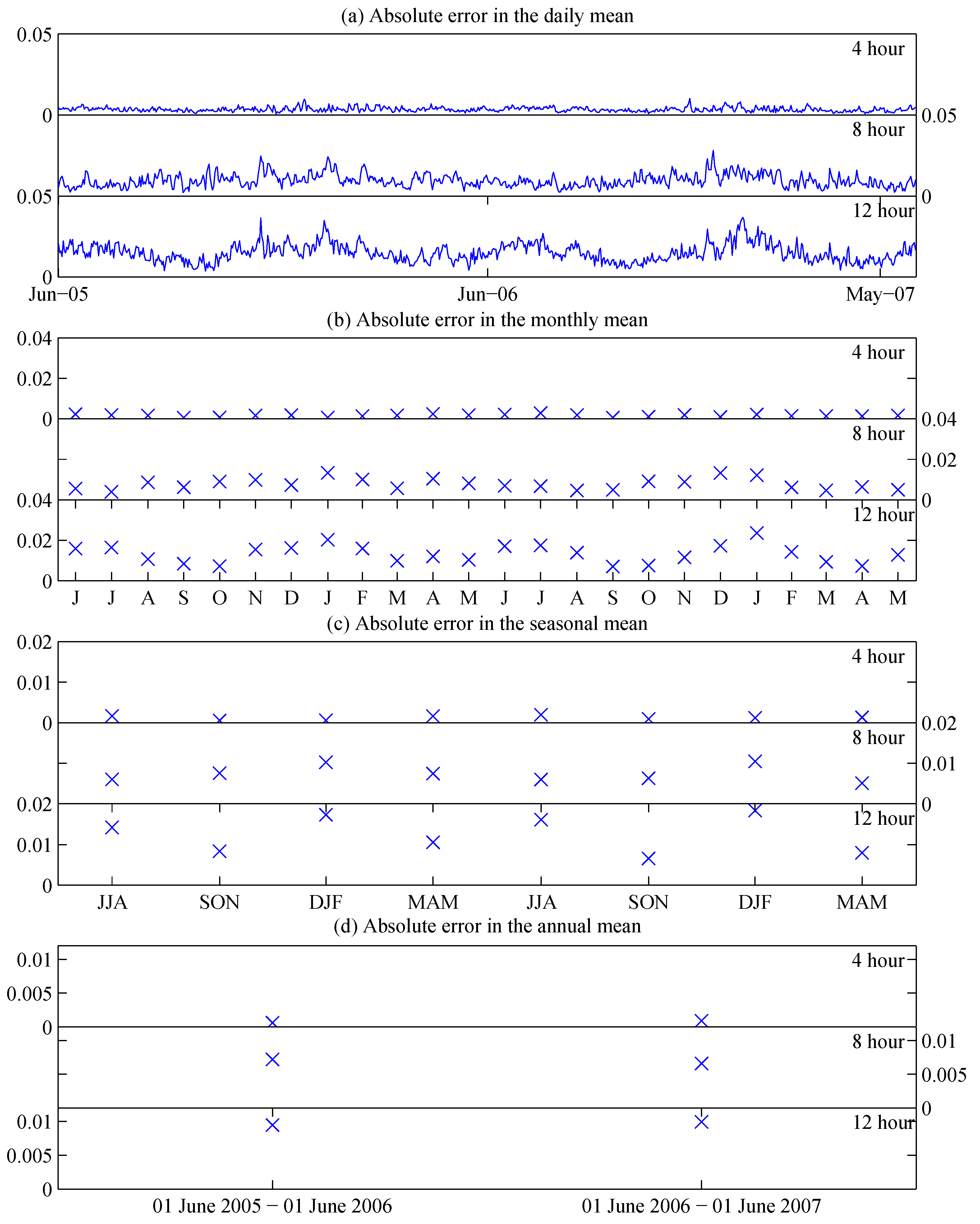
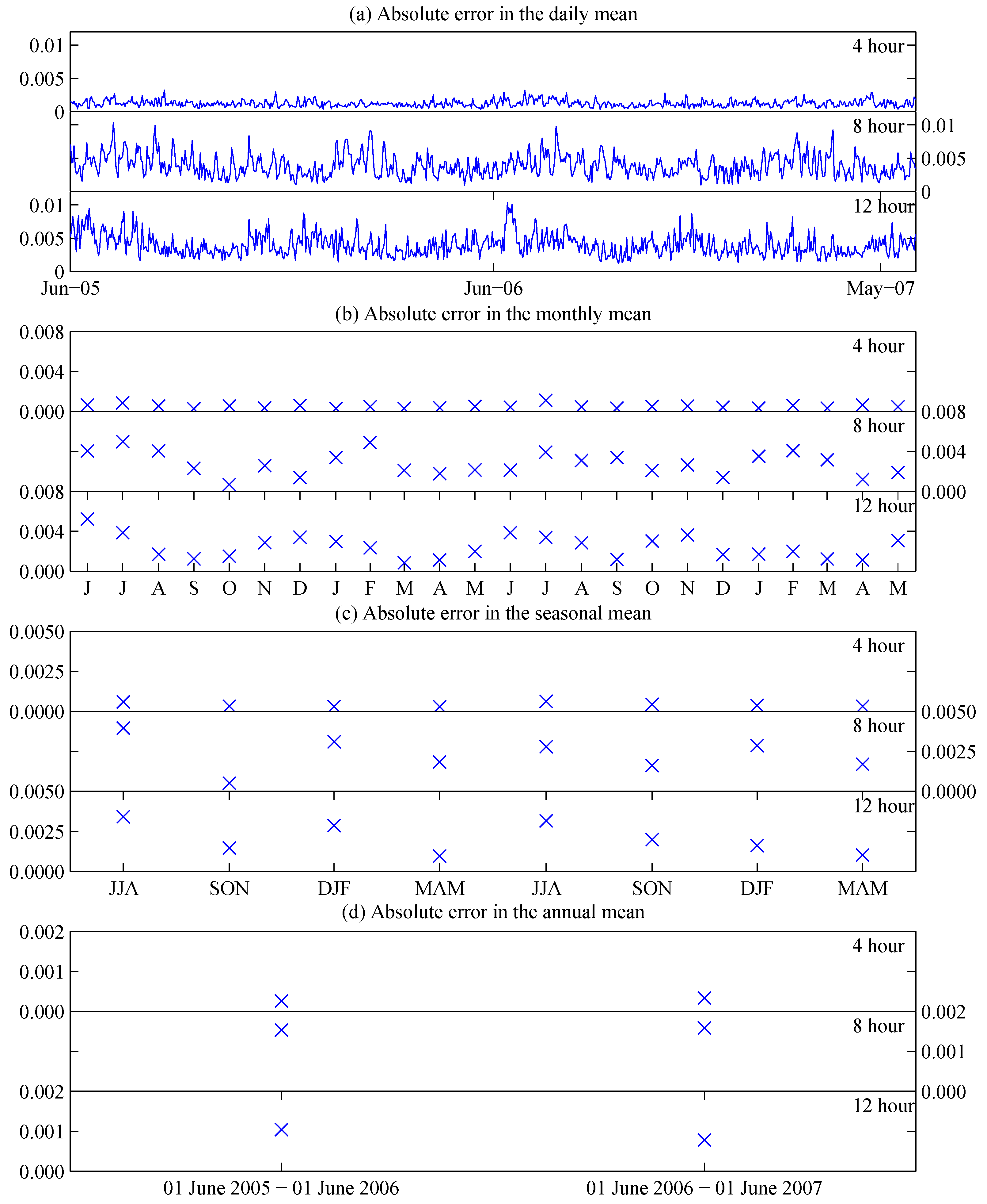
Figure 3 also shows the general trend that the uncertainty increases as the sampling frequency decreases. For the 12-h sampling frequency, the one standard deviation marks are further from the mean. This is confirmed by examining
over land, shown in
Figure 4. Here it is clear that the absolute errors in the means generally increase as the sampling frequency decreases. It is also clear that the uncertainty increases in the northern hemisphere winter months, where the means were seen increasing. Note that, compared to coarser temporal resolutions, when a sampling frequency of 4-h is used the seasonal cycle is significantly less, demonstrating that using this level of sampling rate helps to ameliorate the uncertainty when a smaller area of land is in view.
Generally the behavior seen for cloud fraction in
Figure 3 and
Figure 4 is similar to that seen for radiation in Part-1. A sampling frequency of 4-h or finer results in a smaller uncertainty in the calculation of the sunlit spatial mean. For 4-h sampling, the uncertainty is fairly consistent throughout the year for all periods—daily, monthly, seasonal, and annual.
The Nature Run mean total cloud fraction over land varies between 50% and 60% for the sunlit half of the Earth (
Figure 3). Note that from
Figure 4 the uncertainty in the daily mean is about 1% or smaller for 4-h sampling frequency, 2% for 8-h, and 4% for 12-h sampling. For annual mean, the uncertainty associated with 4-h sampling is 0.1%; it is slightly less than 1% for 8-h and 1% for 12-h sampling. These uncertainty levels are significant for climate studies, where cloud remains a major source of uncertainty in climate forcing [
11]. Studies ([
11] and the rerferences therein) have shown that the net global and annual radiative effect of clouds is about −20 Wm
−2. Assuming a global cloud coverage of 60%, one percent of change in cloud fraction is equivalent to about 0.33 Wm
−2 in radiative forcing, which is comparable to the global aerosol direct radiative forcing (−0.35 Wm
−2) [
12]. Since long term cloud coverage change can either magnify or reduce the CO
2-of great interest. Studies have found that the trend signal is very small. Over the tropical ocean it, is about 1.4% change per decade and over other areas, the signal is even smaller or nonexistant [
13]. The uncertainties shown in the subsampling with temporal resolution coarser than 4-h would have significant impact on the cloud coverage trend study. We do note that in this work, uncertainties from other sources such as those in cloud detection (e.g., [
14,
15]) which can have larger effects are not considered.
Figure 5 is equivalent to
Figure 3, but shows the mean and standard deviation for the sunlit ocean. The mean cloud fraction over the ocean is higher than over land, varying between around 0.65 and 0.7. The difference between the means and the standard deviations appears to be smaller for ocean than land, and this is confirmed by examining the errors in the mean in
Figure 6. For all sampling rates and intervals, the uncertainty in measuring the mean cloud fraction over ocean is smaller. Similar as for land the uncertainty is more consistent throughout the year for the 4-h sampling than seen for the 8-h and 12-h sampling. The Earth’s surface is around two-thirds ocean, so DSCOVR’s view will always contain a significant amount of ocean. This is not the case for land, when at certain times of year only small geographical areas of land are in view. For these smaller regions, variations can be larger due to the large variations of cloud at specific locations. Since small geographical areas of ocean are not encountered, larger associated uncertainty is also not encountered.
Another feature in the above results is that the errors are not always smaller for 12-h sampling frequency
versus 8-h. For the annual means over ocean, the errors are largest for the 8-h sampling frequency. This is different to what has been seen for land cloud fraction and outgoing radiation, where increasing sampling frequency generally resulted in smaller uncertainty. These results are confirmed by examining
for land, ocean, and global regions over all periods, shown in
Figure 7. Each data point in
Figure 7 corresponds to the mean of sets of standard deviations shown in
Figure 3 and
Figure 5, with additional sampling frequencies also shown. For total cloud fraction over land, up to 4-h sampling frequency the mean uncertainty increases quite gradually—especially for monthly, seasonal, and annual means. For sampling frequency of 4-h or greater the uncertainty tends to increase more rapidly. For the ocean region, the results are similar up to 8-h sampling frequency, in that the increase in uncertainty is more gradual from 2-h to 4-h than it is from 4-h to 8-h. The results are very different from 8-h to 12-h though, here the uncertainty actually decreases for all time intervals.
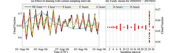
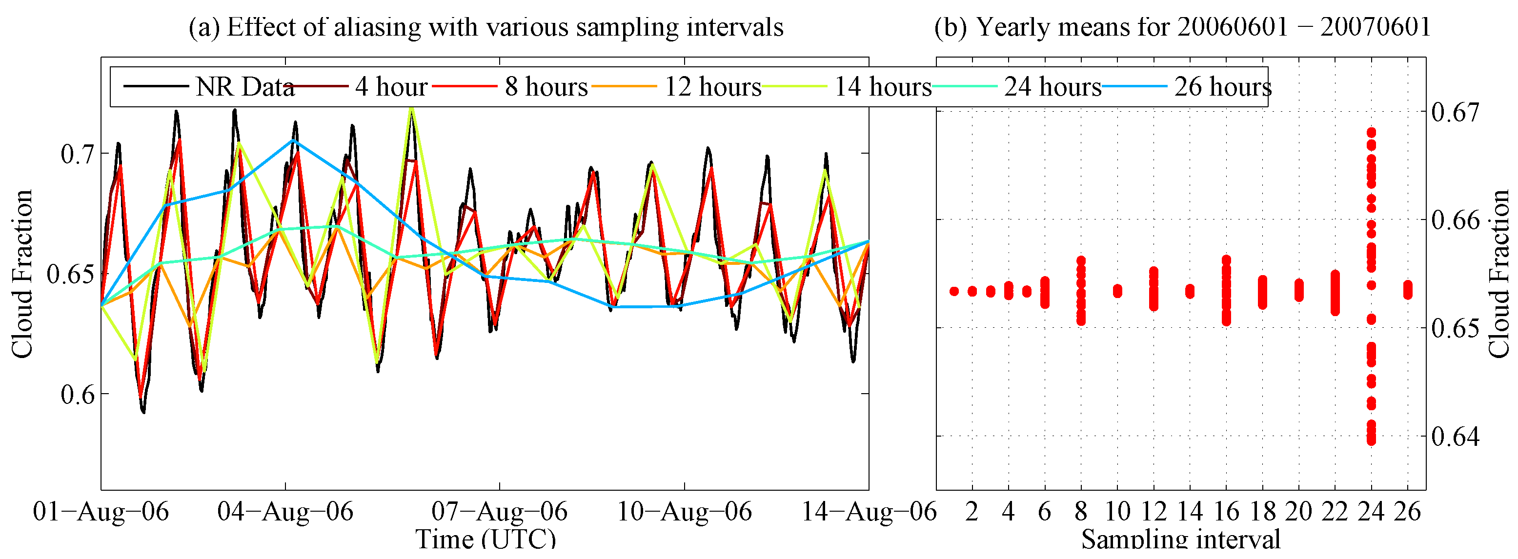
Upon closer inspection, the increase in uncertainty for ocean cloud fraction between 8-h and 12-h sampling frequencies appears to result from an underlying signal within the time series. The issue is demonstrated by considering a sampling frequency of 24-h against other sampling frequencies, for which the problem is magnified.
Figure 8a shows the time series of the mean sunlit ocean total cloud fraction for a two week period beginning 1 August 2006 at 0000 UTC. The figure shows the nature run time series
versus the time series with a selection of sampling frequencies with the same starting point. Examining this small section of the time series it is clear that a highly diurnal cycle is present in the mean sunlit ocean cloud fraction time series. This is different to the normal atmospheric diurnal cycles in the sense that DSCOVR always views the sunlit hemisphere so it is not related to cloud fraction being different during the day
versus at night. Instead this is related to the side of the Earth that DSCOVR happens to be observing. When sampling frequency is below 24-h, all the curves capture the time series variations over this two week period, with varying degrees of aliasing. However, when the frequency is exactly 24-h, only the peaks of the time series are captured and the entire signal is effectively aliased. For this particular starting point, the mean for the two week period is captured very poorly. Indeed, the 26-h sampling frequency does better at capturing the range of possible values than the 24-h. This is because the sampling frequency is different to the period of the underlying signal. The annual means for all starting points and sampling frequencies for the period 1 Jun 2006 at 0000 UTC to 1 June 2007 at 0000 UTC are shown in
Figure 8b. It is clear here that the uncertainty is much broader for the 24-h sampling frequency than any others, including higher frequencies. The figure also demonstrates that the uncertainty is not monotonic as the sampling interval increases. The largest uncertainty is seen for 8-, 12-, 16-, and 24-h sampling frequencies. It should be noted that even though sampling at certain longer time intervals may result in a more certain annual mean than sampling at shorter intervals, information is lost as the sampling interval becomes larger and larger, as will be demonstrated later in the discussion.
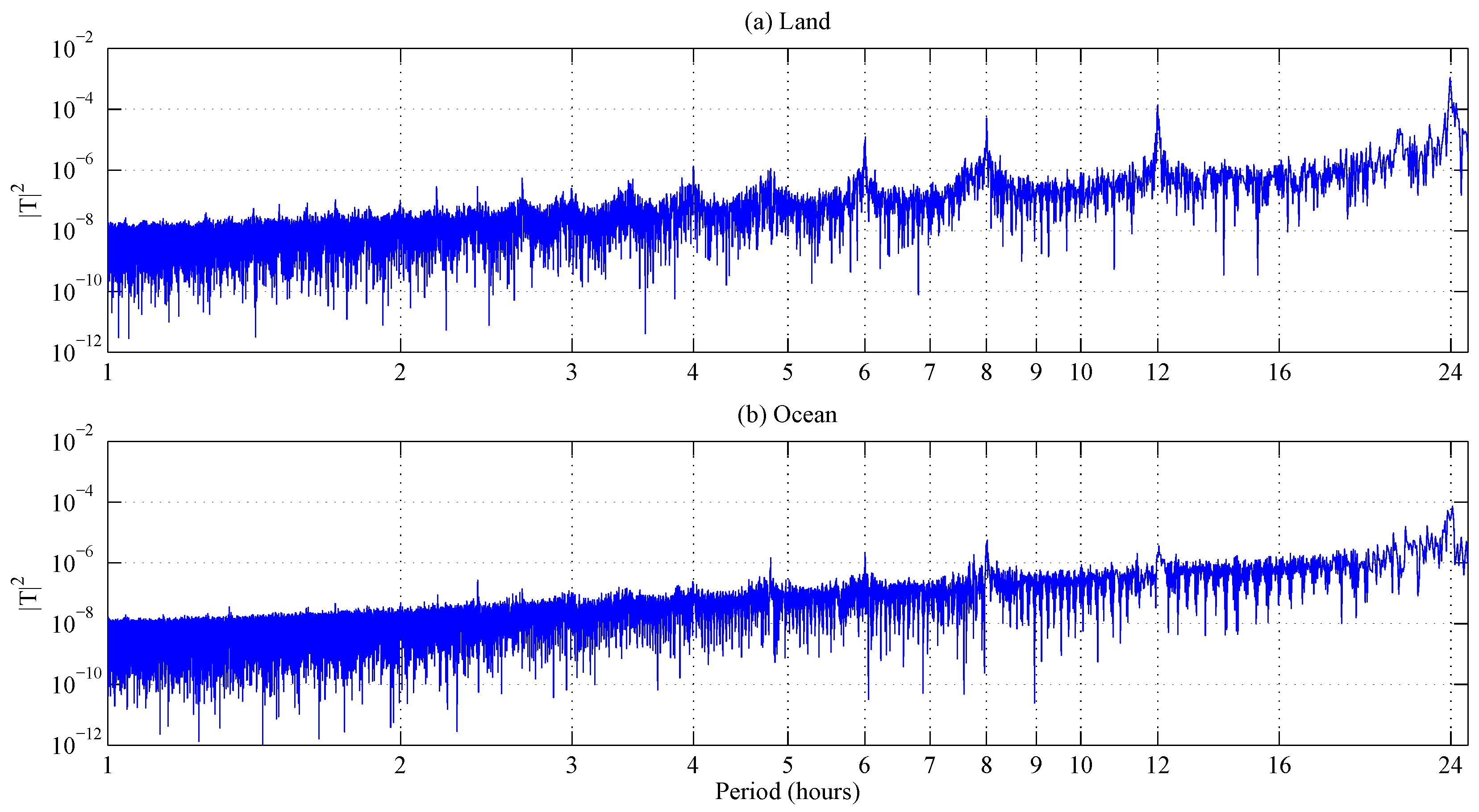
To further understand the varying of uncertainty with sampling frequency, the FFT of the “truth” time series is analyzed.
Figure 9 shows the power spectrum
against period (in hours) for the (a) land and (b) ocean “truth” time series. Only the portion of the spectrum for wavelengths between 1-h and 25-h is shown. The FFT is computed for a six month period from 1 Jun 2006 at 0000UTC to 1 December 2006 at 0000UTC. Peaks in the spectrum highlight where the original time series contains a strong underlying signal. The peak at 24-h in
Figure 9b, for example, correlates with the highly diurnal cycle of ocean cloud fraction that was identified in
Figure 8a. Examining
Figure 9a, it is clear that this diurnal cycle is present in the land region as well. It is not surprising to see such a large signal with a 24-h period, since this matches the orbital period. For frequencies greater than 24 h, there are no additional peaks and the spectrum increases approximately linearly. This is omitted from
Figure 9 to allow focus on the more interesting part of the spectrum. The linear increase in the spectrum throughout appears to result from a so-called red noise in the time series [
8]. The spectrum for a time series of red noise with an autocorrelation coefficient of around 0.95 was examined and found to have a very similar rate of increase as well as structure in the low frequency oscillations.
The results in
Figure 7 show that mean uncertainty was higher over land than over ocean. The magnitude of the spectral coefficients for land are higher than for ocean, and the peaks have more contrast with other wave number signals. Peaks in the land region spectrum occur not just for 24-h but also for 4-, 6-, 8-, and 12-h, which are all shown in
Figure 7a as well. For daily means, it remains true that the finer the sampling frequency, the smaller the mean uncertainty. The reason that the 12-h sampling frequency has smaller uncertainty than that of the 8-h over ocean (
Figure 7b) is because the magnitude of
is larger for 8-h than 12-h.
Given the above results, it is clear that a sampling frequency should be used that does not match peaks in the power spectrum. For computing monthly, seasonal, and annual means of cloud fraction, this means avoiding sampling frequencies of 4-h, 6-h, 12-h, 24-h, and multiples thereof. It has already been noted that a sampling frequency of not more than 4-h should be used for computing daily means.
The results above consider the uncertainty in the period means. Another consideration is the aliasing associated with a particular sampling frequency. This provides insight into the uncertainty in a particular instantaneous measurement. For example if the area mean cloud fraction is computed from DSCOVR, how uncertain is it at a particular moment, rather than over a particular period?
Figure 10 shows the mean
(solid curves) and standard deviation
(dashed curves) of the correlation coefficients for land, ocean, and global regions between the subsamples and the “truth”. Correlation coefficients are computed for daily, monthly, seasonal, and annual intervals then averaged over all of the occurrences of those periods.
The correlation coefficients decrease as the sample frequency becomes coarser. This demonstrates that even though it may be possible to obtain a mean that is close to the “truth”, subsampled time series are farther and farther away from the “truth” as the temporal resolution becomes coarser and coarser. There is little difference among land, ocean, and global regions, demonstrating that the aliasing is similar for each.
4. Conclusions
The time series of cloud fraction on the sunlit hemisphere of Earth as produced by the GEOS-5 high resolution Nature Run has been analyzed in support of the DSCOVR mission. DSCOVR orbits around the Sun–Earth L1 Lagrange point, providing an uninterrupted view of the entire sunlit hemisphere. The aim of this work is to simulate the observations of cloud fraction observed by DSCOVR and to understand how temporal sampling frequency affects the observations.
A set of metrics have been used to analyze the time series of the sunlit mean cloud fraction. These are uncertainty in the mean across a range of possible start times, absolute errors in the mean, and correlation between original and sampled time series. In addition to these metrics, a Fourier spectral analysis of the time series was also conducted.
Cloud fraction was examined over land and ocean separately. Generally it was found that using a sampling frequency finer than 4-h resulted in small uncertainties. Over ocean, the uncertainty in annual mean cloud fraction decreased when using 12-h sampling frequency versus 8-h, which was caused by an underlying signal in the time series with a period of 8-h. Fourier analysis revealed a number of strong underlying signals, notably with 6, 8, 12, and 24-h periods (all integer factors of 24). Comparing with other results, it is shown that uncertainty can be significantly higher when the sampling frequency matches these periods. To achieve accurate results on the means, DSCOVR needs to avoid sampling frequencies that correlate with peaks in the power spectrum.
Analysis of correlation coefficients between the subsamples and the “truth” shows that even though subsampling at certain longer time intervals may not increase the uncertainty in the mean significantly, the subsampled time series are further and further away from the “truth” as the sampling interval becomes larger and larger. These results provide helpful insights for DSCOVR’s temporal sampling strategy.


