Article

Mapping Paddy Rice in China in 2002, 2005, 2010 and 2014 with MODIS Time Series

1
Department of Remote Sensing, Institute of Geography and Geology, University of Wuerzburg, Oswald-Kuelpe-Weg 86, D-97074 Wuerzburg, Germany
2
Institute of Geographic Sciences and Natural Resources Research, Chinese Academy of Sciences, 11A Datun Road, 100101 Beijing, China
3
German Remote Sensing Data Center (DFD), Earth Observation Center (EOC), German Aerospace Center (DLR), Oberpfaffenhofen, D-82234 Wessling, Germany
*
Author to whom correspondence should be addressed.
Submission received: 4 March 2016 / Revised: 3 May 2016 / Accepted: 9 May 2016 / Published: 23 May 2016

Abstract

:
Rice is an important food crop and a large producer of green-house relevant methane. Accurate and timely maps of paddy fields are most important in the context of food security and greenhouse gas emission modelling. During their life-cycle, rice plants undergo a phenological development that influences their interaction with waves in the visible light and infrared spectrum. Rice growth has a distinctive signature in time series of remotely-sensed data. We used time series of MODIS (Moderate Resolution Imaging Spectroradiometer) products MOD13Q1 and MYD13Q1 and a one-class support vector machine to detect these signatures and classify paddy rice areas in continental China. Based on these classifications, we present a novel product for continental China that shows rice areas for the years 2002, 2005, 2010 and 2014 at 250-m resolution. Our classification has an overall accuracy of 0.90 and a kappa coefficient of 0.77 compared to our own reference dataset for 2014 and correlates highly with rice area statistics from China’s Statistical Yearbooks (R2 of 0.92 for 2010, 0.92 for 2005 and 0.90 for 2002). Moderate resolution time series analysis allows accurate and timely mapping of rice paddies over large areas with diverse cropping schemes.

Graphical Abstract

1. Introduction

China is the world’s largest producer and importer of rice with a national rice production of 208 million tonnes, 28% of the global production, and a rice import surplus of 2.2 million tonnes [1,2]. Rice is the most important food crop in China, consumes vast amounts of irrigation water and fertilizer and produces green-house relevant methane emissions. Knowledge about the amount and location of rice paddy fields is therefore of dual significance: for food security and policy making in China, as well as for global climate change. Rice is mostly cultivated on small paddy fields with crop cycles that can differ every year, which, combined with the vast amount of fields, makes the collection of current data based on agricultural census a labor-intensive and slow process. Remote sensing methods can help to deliver rice maps that are accurate, cost-effective to produce and more timely than agricultural census data.
Remote sensing of rice with optical satellite sensors exploits the phenological development of the rice plant throughout its life-cycle. It is commonly divided into the vegetative, the reproductive and the ripening phases. The vegetative phase consists of the germination, seedling, tillering and stem elongation stages. The second phase includes panicle initiation, heading and flowering. Ripening is the last phase and includes the milk, dough and mature grain stages. Before transplanting of the rice seedlings, paddies are usually flooded with water. After transplanting, the rice seedlings undergo a rapid growth and greening during the reproductive phase, which culminates at the heading stage. During the last phase, the plants’ leaf density decreases until harvest [3]. All of these changes in plant morphology throughout rice plants’ life-cycle influence their interaction with waves in the visible light, infrared and microwave spectra and, therefore, produce discernible changes in time series of remotely-sensed data [4,5]. In order to distinguish rice from other land cover, especially other crops, time series analysis of multi- or hyper-temporal data has been the most prolific technique. Rice is dominantly grown in precipitation-rich environments with regular cloud cover. Authors of remote sensing-based rice area studies therefore emphasize the need for dense time series and employ data from microwave sensors [6,7,8,9,10,11,12], which are only sparsely affected by clouds, use optical sensors with high revisit times to gather a sufficient amount of cloud-free observations [13,14,15,16,17,18,19] or a combination of both [20,21,22]. Two optical sensors that have been widely used for rice area mapping are MODIS (Moderate Resolution Imaging Spectroradiometer) and SPOT-VGT (Satellite Pour l’Observation de la Terre-Vegetation) due to their long standing archives, data acquisition in the visible light, as well as infrared ranges and high revisit times. Most studies using these sensors detected flooding events followed by rapid vegetation growth, which is regarded as a distinctive temporal feature of paddy rice. Remote sensing studies exploiting this temporal feature have mostly been conducted with decision-tree classifications that employed the combination of different vegetation and water indices and auxiliary data, such as crop calendars, land surface temperature or precipitation [13,23,24]. Studies that focused on the complete temporal signal of rice classified rice areas using wavelet filters [25,26], empirical mode decomposition [27,28] or dynamic time warping [29,30] have also been undertaken.
A number of studies have been performed in China using optical satellite sensors to map rice paddies. A small amount of remote sensing studies have been published that mapped rice areas at the national scale with the majority of studies focusing on mapping at the regional scale in different key regions in northern or southern China. One of the first products was published by Frolking et al. [31], who combined agricultural census data with a Landsat-derived land cover map to generate a rice map for mainland China with a 0.5° resolution. Xiao et al. [23] used MODIS data to generate a paddy rice map for southern China at 500-m resolution based on a method that detects flooding of the paddies with a temporary inversion of vegetation and water index values. Sun et al. [32] employed a similar method with the addition of regionalized crop calendars to produce a 500-m rice map based on the MOD09A1 dataset for China. Qiu et al. [33] developed a method comparing the amplitudes of a water and vegetation index and found that rice areas have lower change ratios of these amplitudes from the tillering to the heading stage. Applying this method to southeast China, they reported a reduction in rice-planted areas of 30% from 2001–2013 with double-cropped rice areas showing a 49% decrease [34]. For the Yangtze Delta region, Shi and Huang [35] mapped rice at 500-m resolution based on a spectral index using the green and mid-infrared MODIS bands and reported a stable total planting area of rice with conversion from double to single cropping in some regions. Xiao’s rice mapping approach has also been demonstrated to work with Landsat data at 30-m resolution with case studies in the Yangtze-Huaihe Plain [22] and the Sanjiang Plain [36]. Wang et al. [37] showed that data from the Chinese Huanjing-1 (HJ-1) A/B satellites can also be used to map rice in the fragmented agricultural areas of the Hangjiahu Plain. During the last two centuries, rice production in northern China continually increased due to food demand and the effects of changing climate. This emerging rice region has been examined in a number of studies. The well-known vegetation-water-index-inversion approach was applied on MODIS data to map rice in northeast China at 500-m resolution for the years 2001–2009 [38]. Zhou et al. [39] integrated Landsat 8 data with MODIS Land-surface temperature data to map rice in the Panjin Plain for 2013 at 30-m resolution. FORMOSAT-2 images and a maximum-likelihood classifier were used by Zhao et al. [40] to map rice in Qixing Farm County at 8-m resolution for 2009. Recent studies employ time series analysis of Landsat images to map rice at the regional scale [41]. Dong et al. [42] developed a Landsat-based rice classification and land cover change detection system, which they showed to work by classifying rice planting area at the Chinese-Russian border for five epochs between 1986 and 2010 and reported a twenty-fold increase in paddy rice area. This approach was also shown to work at a larger scale by classifying rice areas in northeast China, North and South Korea and Japan [43].
Except for approaches focusing on rice seasonality mapping, classifying rice can be regarded as a binary classification task with the two classes rice and no_rice. The distribution of both classes is inherently imbalanced due to the large size and diversity of the no_rice class. The imbalance of the training set is an issue that not all supervised machine learning algorithms handle well [44]. Most large-scale rice classification studies to-date used classification techniques based on the phenological development of the rice plant and the resulting spectral responses. Support Vector Machines (SVMs) offer a framework that works well with limited amounts of training data and uneven class distribution and, as such, are a viable and well-studied tool in land cover classifications based on remotely-sensed data [45]. SVMs sparked a number of methods for one-class classification and outlier detection, such as support vector data description [46], biased SVM [47] and one-class SVM [48,49]. In this study, we employed a one-class classification approach using MODIS-derived time series data to map all rice paddies in mainland China.
To our knowledge, there are no products available that map paddy rice area in mainland China using MODIS data at 250-m resolution and a concise classification method. Therefore, the objectives of this study are to:
  • develop a method to classify paddy rice areas in the entirety of mainland China based on MODIS-derived time series using a one-class classifier;
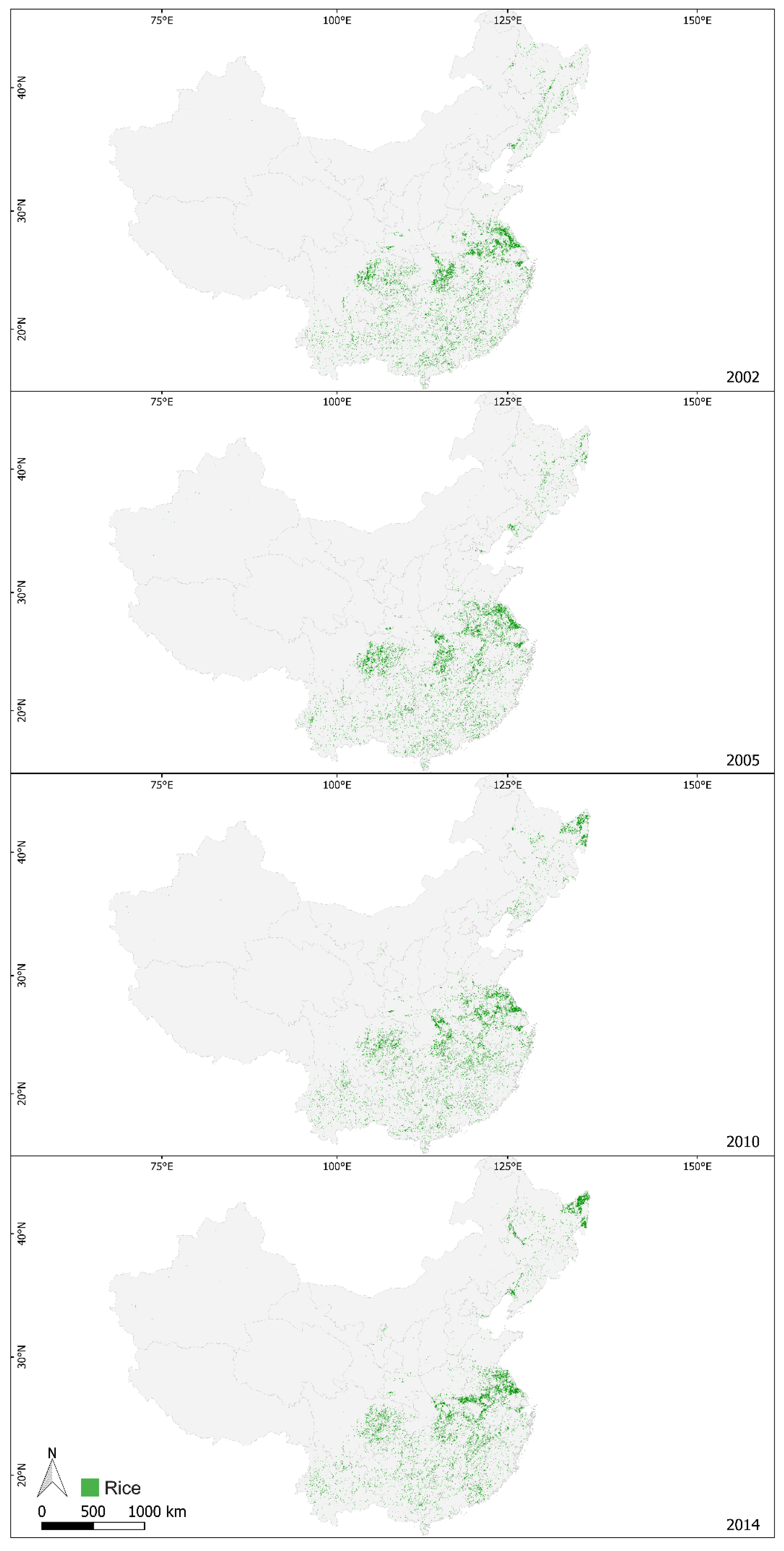
  • create maps of paddy rice areas in mainland China for the years 2002, 2005, 2010 and 2014 and validate their accuracy with reference datasets;
  • analyze changes in China’s paddy rice area from 2002–2014.

2. Study Area: Mainland China

Our study area is mainland, or continental, China and extends from 73°–135°E and 18°–54°N. It covers an area exceeding 9 million km2 and, due to its size and topography, a diverse range of climates from the desserts in the west, the winter-cold regions with fertile soils in the north, to the hilly regions with high temperatures and favorable precipitation in the south and southeast. Throughout these diverse regions, China has about 120 million ha of agriculturally-used land of which 20%–30% is used for paddy rice production [2,50,51,52]. Paddy rice cultivation is practiced in all provinces, except Qinghai, with Hunan, Heilongjiang and Jiangxi being the biggest producers of rice and contributing 33% to the total production of 208 million tonnes for the year 2014 (see Figure 1) [2]. Most of the paddy rice areas are located along large fluvial plains and river deltas due to their fertile soils, flat topography and access to enough water to regularly flood the paddies. Prominent rice regions are the Sanjiang Plain in Heilongjiang, the Yangtze River Delta, the plains surrounding Dongting Lake, but also the hilly regions of the Sichuan, Jiangxi and Guangxi provinces, where rice terraces with limited access to farm machinery are actively cultivated. In provinces with favorable climate multi-cropping, the growing of multiple crops in succession throughout one year is practiced. The cropping intensity gradually increases from one crop in the northern provinces to up to three crops per year in the southern provinces [53], with the boundaries closely resembling China’s different climate zones. North of the Yangtze River and in the westernmost provinces, only one season of rice per year is cultivated. South of the Yangtze is a zone of transition with one long or two short rice seasons. Further south, starting around the Nanling Mountains, mostly two rice crops are cultivated per year due to an abundance of rainwater, moist soils and high temperatures year-round [32,54]. Rice can be planted in a variety of cropping schemes, such as rice-rice, rice-vegetables, rice-soybean, winter wheat-rice or rice-rice-alfalfa [31].

3. Data and Methods

3.1. MODIS Data

MODIS is one of the key instruments aboard the Sun-synchronous Terra and Aqua satellites. For our study, we used the vegetation index products MOD13Q1 and MYD13Q1 Collection 6 [55,56]. The products contain 12 layers at 250-m spatial resolution, of which we used the Normalized Difference Vegetation Index (NDVI), Enhanced Vegetation Index (EVI), red (620–670 nm), Near-Infrared (NIR, 841–875 nm), blue (459–479 nm), Mid-Infrared (MIR, 2105–2155 nm) and pixel reliability layers. The 16-day composites have been derived from the atmospherically-corrected eight-day composite products MOD09A1 and MYD09A1, which themselves have been generated from the daily reflectance products based on the constrained view angle maximum value composite technique and corrected for gases, clouds and aerosols [57,58,59,60]. Only the red and NIR band were originally acquired at 250-m spatial resolution, whereas the other surface reflectance bands were acquired at 500-m spatial resolution and resampled to 250-m for the MOD13Q1 and MYD13Q1 products.
MODIS datasets are delivered in sinusoidal projection and a tiling system, where each tile covers an area of approximately 1,440,000 km2. Continental China is covered by the tiles H25V03, H26V03, H23V04, H24V04, H25V04, H26V04, H27V04, H23V05, H24V05, H25V05, H26V05, H27V05, H28V05, H25V06, H26V06, H27V06 and H28V06. For each year and tile, 46 MOD13Q1/MYD13Q1 products were available, except for 2002, for which 35 products were available due to the Aqua satellite being launched in May 2002. We acquired all available MOD13Q1 and MYD13Q1 products for these tiles and the years 2002, 2005, 2010 and 2014 from the USGS Data Pool [61]. We chose the years 2002 and 2014, as they were the first and last years with available MOD13Q1 and MYD13Q1 at the time of our study, and the years 2005 and 2010, due to their alignment with the creation of China’s National Land Cover Dataset.
We extracted all surface reflectance and vegetation index layers from the datasets and created an additional Land Surface Water Index (LSWI2130) from the near-infrared and mid-infrared layers with the equation:
L S W I 2130 = NIR MIR NIR + MIR
where NIR is the Surface Reflectance Band 2 with a wavelength from 841 nm–876 nm and MIR is the Surface Reflectance Band 7 with a wavelength from 2105 nm–2155 nm, centered on 2130 nm. Using the pixel reliability layer, we masked all values that are not classified as Good Data, therefore excluding data classified as Marginal Data, Snow/Ice or Cloudy. Throughout our processing chain, the MODIS data were kept in the original sinusoidal projection.

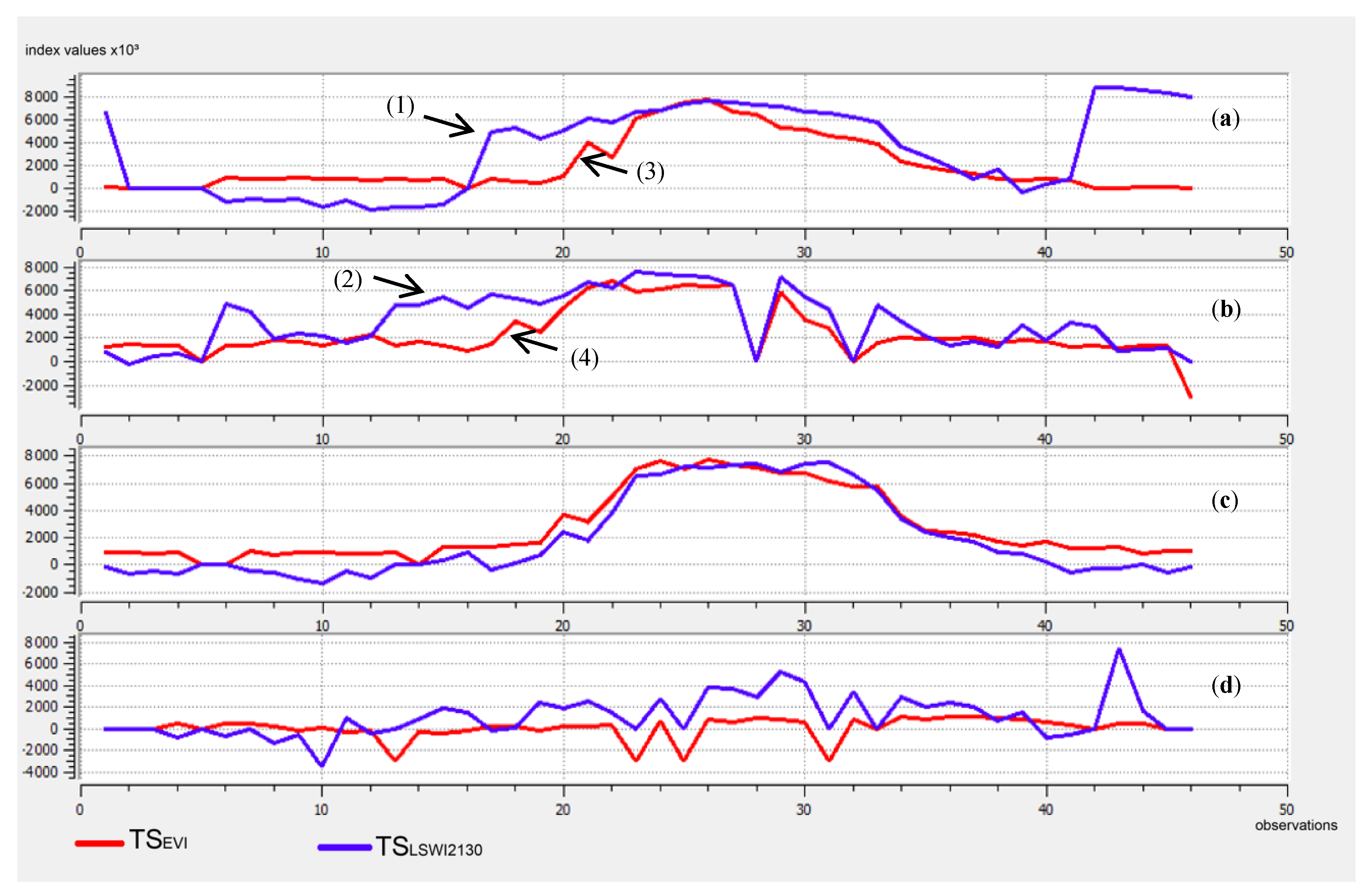
3.2. Time Series Creation and Feature Extraction

The two MODIS 16-day composites are delivered with an eight-day shift between them, which we used to combine both into synthetic time series with eight-day intervals spanning 46 observations and alternating MOD13Q1 and MYD13Q1 data. This approach introduces the issue that pixel values from one scene might be from a later day of the year than the one of the following scene. With the compositing algorithm used to generate the MODIS products, this is seldom the case; however, we still decided to derive metrics from the time series that are mostly independent of these possible temporal overlaps. Calculation of the local extrema is influenced by this error source; therefore, we decided to use only their sum as a feature in our classification and disregard their temporal position in the time series. This approach is different to most time series-based rice classifications, which capitalize on the temporal position of distinctive water or vegetation index peaks. Each layer has been stored in its own Time Series (TS), denoted as TSNDVI, TSEVI, TSred, TSNIR, TSblue, TSMIR and TSLSWI2130. From these time series, we extracted the following features as the input of our classification (Table 1).
All features were calculated along the temporal axis of the time series. The percentiles were defined as the value in the time series below which the given percentage of observations fall. The amplitude was calculated as the difference between the largest and the smallest value in a time series. Prior to the calculation of the local maxima and minima, the gaps in the time series, resulting from the pixel reliability mask, have been linearly interpolated. Should the temporal gap exceed three consecutive values, no interpolation and smoothing were applied. In the next step, TSEVI was smoothed with a Savitzky–Golay filter with a window length of five (including the center value) and a second order polynomial, which is commonly applied in time series analysis of vegetation indices [62]. The interpolated time series were used as input for the local extrema calculation. Local maxima have been defined as the values in the time series that are larger than the three observations prior and the three observations after them while also exceeding the given threshold. Local minima are the inverse and have to be below the given threshold. The amount of observations along the temporal axis that fulfill these criteria was then counted. The EVI and LSWI2130 inversions have been defined as the amount of observations where the value of the TSEVI exceeds 0.45 and double the value of TSLSWI2130. This feature is similar to the EVI-LSWI inversion rice classification approach employed by Xiao et al. [13,23,24], although they calculated LSWI with the short-wave-infrared band with a wavelength from 1628 nm–1652 nm, which is not available in the MOD13Q1/MYD13Q1 datasets. In total, we calculated 64 features from our input time series giving special consideration to the features being robust in regard to the possible temporal overlap in our synthetic eight-day time series.

3.3. Reference Datasets

We created a reference dataset for rice paddies based on very high resolution satellite images and our aforementioned EVI and LSWI2130 time series. Training areas were selected that are distributed over the different rice growing regions of China with the goal to incorporate all major rice growing schemes in regards to crop calendar, length of the growing season, multi-cropping, temperature and precipitation regimes, as well as different paddy types, such as terraces, large uniform farms and small and scattered fields interspersed with other crops and land cover. We selected 25 training areas (Figure 2). We also had access to data from Agricultural Meteorological Stations (AMSs) for the year 2002, which have been operated by the Chinese Meteorological Agency and have previously been used to derive the multiple cropping intensity of China’s agriculture [63]. The subset we were able to use includes information about key crop growth phases of rice plants, such as planting, emergence and maturity dates, of 126 rice paddy fields, as well as the location of the AMSs (Figure 2).
For each training area, we drew a bounding box, inside which we delineated rice paddies as the class rice, as well as all other land cover types and agriculture as the class no_rice. The size of the bounding boxes is 12 km by 12 km. An exception are three training areas with small rice terraces in Sichuan, Guangxi and Yunnan provinces where the size is 6 km by 6 km. The delineation of the land cover polygons, meaning areas of equal land cover, was based on very high resolution imagery from the WorldView, Ikonos and Spot satellite constellations for the year 2014 available through virtual globe software Google Earth, as well as MapWorld. When an image from 2014 was not available, we used imagery from 2013 or 2015 on the basis that paddy field boundaries are not usually subject to sudden change.
For each paddy polygon, we decided to classify it as rice or no_rice based on the interpretation of the temporal profiles of TSEVI and TSLSWI2130, since rice is difficult to distinguish from other crops in mono-temporal imagery. Most paddy fields are flooded prior to transplanting rice seedlings, resulting in a peak of the water index prior to a steep rise in the values of the vegetation index. This creates temporal profiles for these indices that are unique to rice and have been successfully employed for its classification [7,13,25,42]. An early peak of TSLSWI2130 just before a steep rise in TSEVI, as the distinctive temporal feature of paddy rice, becomes apparent when it is compared to other crops and land cover (Figure 3). The temporal profiles of the water index in Figure 3a, near Lake Xingkai, Heilongjiang, and Figure 3b, near Lu’an, Anhui, show a clear and sudden rise resulting in a peak (a-1, b-2) before the vegetation index starts to rise (a-3, b-4). This is a clear indicator of the flooding of the paddies before rice is transplanted and subsequently grows, resulting in the sharp increase in TSEVI. If a paddy in one of our training areas exhibited this behavior, we classified it as rice; otherwise, it was classified as no_rice. The rice class therefore contains fields with at least one discernible rice crop per year. Rice is hard to distinguish from other crops in a mono-temporal satellite image, but their differences become clear when comparing the temporal profiles of (a) and (b) in Figure 3 to the example (c), a corn field in Tianin province at Bohai Bay, as well as example (d), an assembly of aquaculture ponds at Dongting Lake.
With this method, we created a total of 2132 rice polygons and 471 no_rice polygons in our 25 training areas. In order to train and select a model, as well as determining its accuracy on independent data, the reference data have to be split. We followed the recommendations by Hastie et al. [64] and performed a 50/25/25 split on the rice class and a 50/50 split on the no_rice class. The splits were performed on the polygon level to minimize the effects of spatial correlation. We randomly split the rice polygons into 50% used for training of the model, 25% used for model selection and 25% for accuracy assessment. No data for training the model were necessary from the no_rice class, so we split it into 50% used for model selection and 50% for accuracy assessment. For the training, selection and validation of our model, we used all MODIS pixels where the centroid was located inside one of the polygons, resulting in a total of 27,384 useable pixels for the rice and 26,936 for the no_rice class.
Additionally we acquired agricultural census data at the province level from China’s Statistical Yearbooks [2,50,51,52]. The basis for this data is the censuses at the county and township level, which are collected by Statistical Bureaus at the province level, as well as reports by state-owned farms collected by the Bureau of Reclamation. These data are compiled into Statistical Yearbooks by the National Bureau of Statistics of China [2]. The data we used were Output of Rice, Total Sown Area of Rice for the years 2014, 2010, 2005 and 2002, as well as Sown Area of Early Rice, Sown Area of Middle-season Rice and Single-Cropping Late Rice and Sown Area of Double-Cropping Late Rice for the years 2010, 2005 and 2002. The province names used throughout this paper have been taken from China’s Statistical Yearbooks, and the province boundaries have been extracted from the Global Administrative Areas dataset [65].

3.4. One-Class Support Vector Machine

One-Class Support Vector Machine (OCSVM) [48] is a supervised, one-class classification method based on the SVM framework. It only requires training data from the target class and, when used with the Radial Basis Function (RBF), the setting of two parameters: ɣ and ν. Like other SVMs, it uses a kernel function to map samples into a higher dimensional feature space. In a binary SVM, a hyperplane is then generated that seeks to maximize margins between the hyperplane and the closest training samples. The separating hyperplane is the decision boundary between the two classes, and the closest training samples are the vectors supporting it. In an OCSVM, the decision boundary tries to delineate the samples of the target class from the origin in the mapped feature space. The ɣ parameter determines the width of the RBF kernel, whereas ν is the lower limit of the amount of support vectors and the upper limit of the fraction of training samples that are classified as outliers. Tuning of the parameters is usually more difficult than in other SVMs due to the unavailability of samples from the outlier class [66].
For our OCSVM model, we scaled all input samples by scaling to unit variance and removing the mean, so that no feature can dominate the learning and classification process. The classification was performed using the scikit-learn package (see Appendix A). We chose to collect samples from the target, as well as from the outlier class to overcome the OCSVM parameter selection problem and perform a grid search to select the optimal values. A grid search was performed using 25% of our rice and 50% of our no_rice reference data. As the optimization criterion, we chose the f1-score as a balanced measure between recall and precision, which is an appropriate measure for imbalanced classification tasks [66], and the RBF kernel, which is a standard kernel suitable for classification tasks [45,67]. The best set of parameters for the RBF kernel was determined with a parameter grid of 200 linearly-spaced ɣ values ranging from ɣ = [0.025, …, 0.5] and ν values ν = [0.05, 0.075, 0.1, 0.125, 0.15], which resulted in a grid search over 1000 parameter combinations. The model with the best performance was then used to classify paddy rice areas throughout China for the years 2002, 2005, 2010 and 2014. The resulting classifications are referred to as OCSVM2002, OCSVM2005, OCSVM2010 and OCSVM2014, respectively, and have a value of one where paddy rice was detected as at least one crop during that year and a value of zero for all remaining pixels, including masked ones.

3.5. Accuracy Assessment

We performed an accuracy assessment with each reference dataset available, resulting in three assessment groups: comparison to our own reference data based on very high resolution satellite images, comparison with agricultural statistics at the province level and comparison with the AMS field measurements. For the first group, we used 25% of our reference rice polygons and 50% of the reference no_rice polygons. We extracted all OCSVM2014 pixel values where the pixel centroid is located within one of the polygons and counted the number of correctly- and incorrectly-classified pixels for each class. From this, we derived a complete confusion matrix and the accuracy metrics overall accuracy, producer’s and user’s accuracy, precision, recall, f1-score, kappa-coefficient and the Matthews correlation coefficient [68,69,70,71].
In the second assessment group, we compared the paddy rice areas derived from our classification to the areas published in China’s Statistical Yearbooks corresponding to the same year as our classification. For each province and year, we counted the number of pixels classified as rice and derived their area based on the exact spatial resolution of our MODIS pixels. The pixel size of MODIS is commonly referred to as 250 m, but the actual pixel size in our datasets is 231.66 m. China’s Statistical Yearbooks do not contain a category for “total paddy area”; therefore, we compared the areas from our classifier to the reported Sown Area with the largest extent to minimize errors arising from multi-cropping where more than one season of rice is planted on a paddy field. Additionally, we also performed the same analysis using provinces where only one rice season is reported or the largest reported season accounts for more than 95% of the Total Sown Area. Provinces where the reported Total Sown Area is equal to the total area of rice paddies, to within 5%, are Beijing, Chongqing, Gansu, Guizhou, Hebei, Heilongjiang, Henan, Inner Mongolia, Jiangsu, Jilin, Liaoning, Ningxia, Qinghai, Shaanxi, Shandong, Shanghai, Shanxi, Sichuan, Tianjin, Tibet, Xinjiang and Yunnan [50,51,52]. These assessments where performed for the years 2010, 2005 and 2002 due to the seasonal data for the year 2014 not being published yet.
In the last assessment group, we extracted the locations of the agricultural meteorological stations as point measurements on the grounds that each AMS was located inside a rice paddy. We then extracted the pixel value of OCSVM2002 in which these points are located and calculated the accuracy.

4. Results

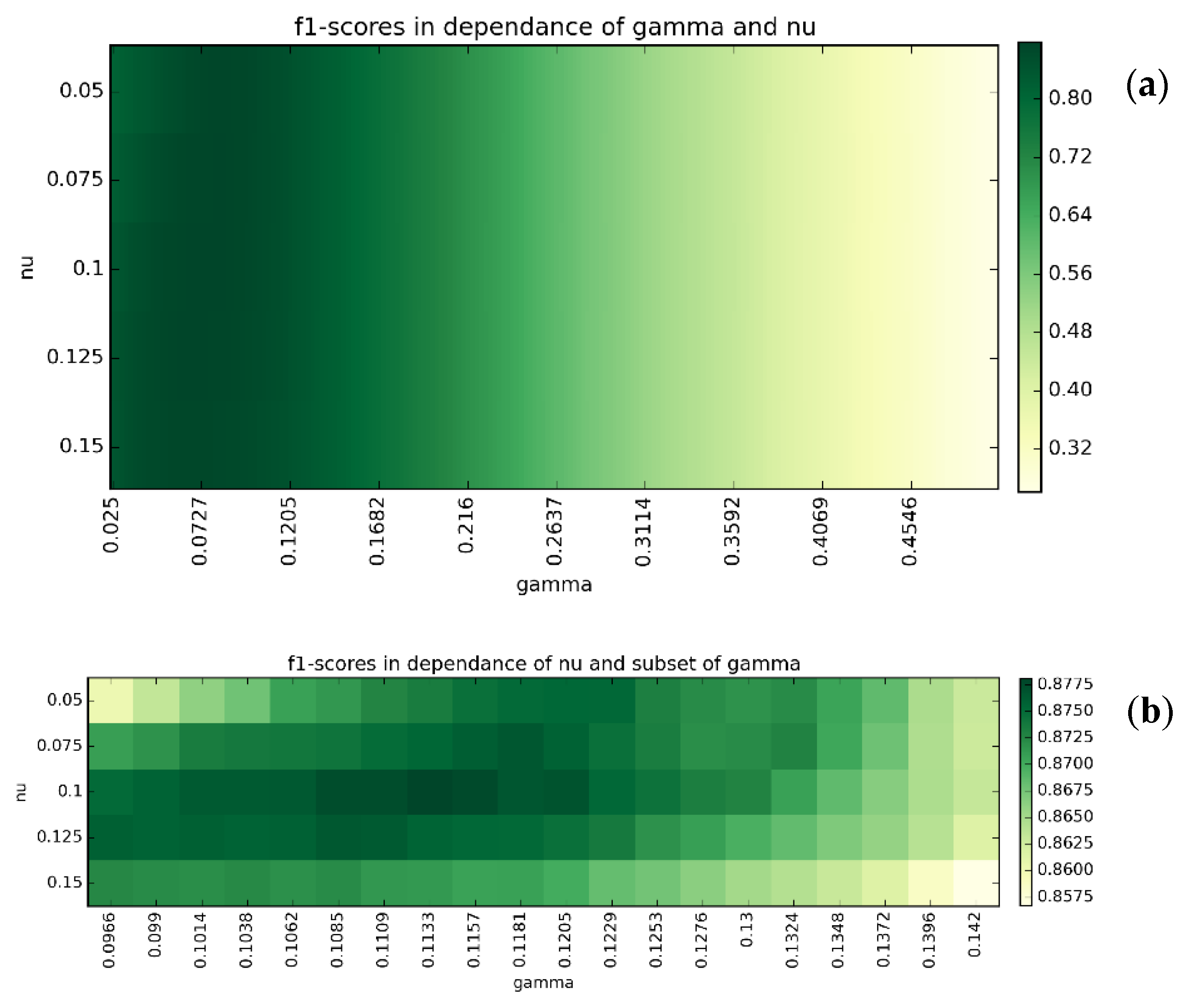
4.1. One-Class Support Vector Machine Model Selection

Our parameter grid search revealed that the parameter values with the best f1-score for our classification task are ν = 0.1 and ɣ = 0.113 for an OCSVM with an RBF kernel. The f1-scores for all ν and ɣ combinations from the grid search are shown in Figure 4a. Figure 4b shows a subset of ν and ɣ combinations around the one with the highest overall f1-score, which we selected as our final OCSVM model parameters.

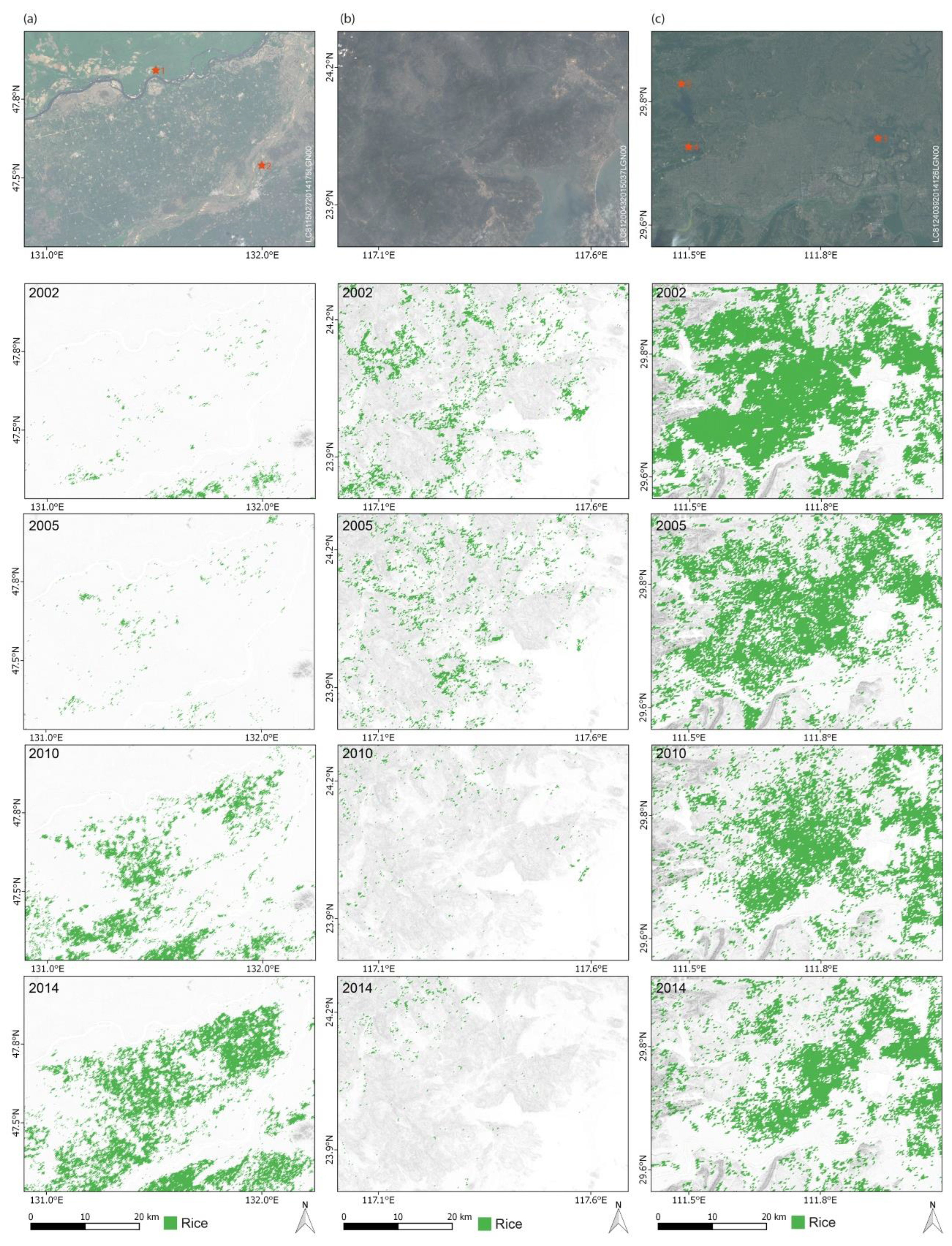
4.2. Paddy Rice Classification

Based on yearly MODIS time series and our trained OCSVM model, we classified paddy rice areas in mainland China at 250-m MODIS resolution for the years 2014, 2010, 2005 and 2002 (Figure 5).

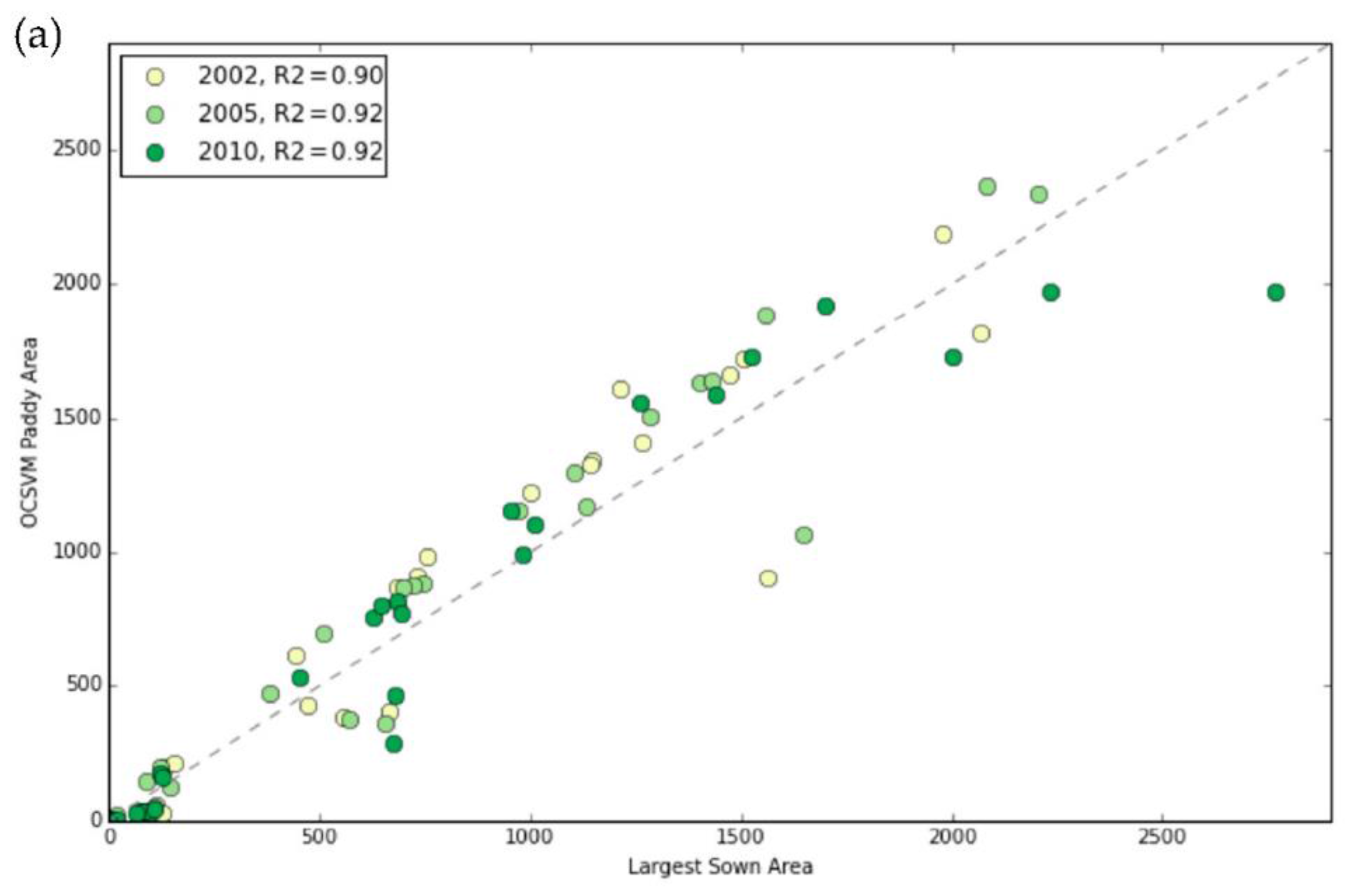
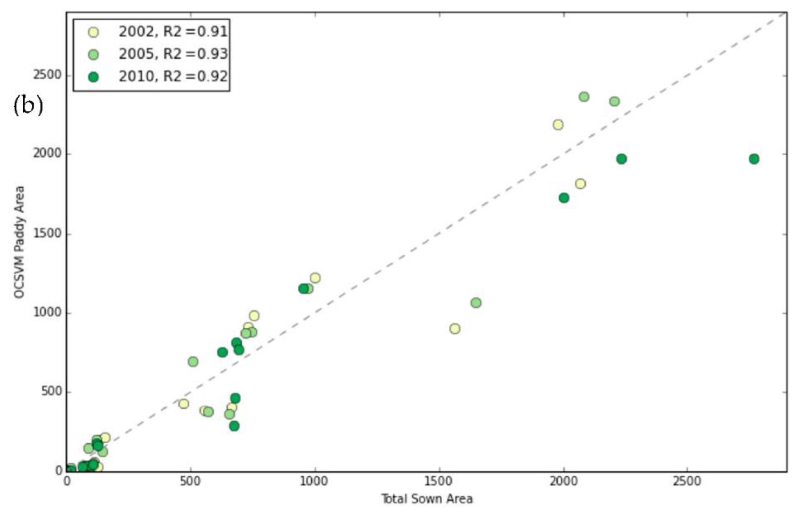
4.3. Accuracy Assessment

For the year 2014, we compared the classification results of OCSVM2014 to our own reference dataset and calculated a confusion matrix (Table 2). We used 25% of the rice and 50% of the no_rice polygons from the reference dataset. From the confusion matrix, we can calculate an overall accuracy of 0.90 and a user’s accuracy of 0.90 for the no_rice and 0.89 for the rice class. The producer’s accuracy is 0.89 for the no_rice and 0.79 for the rice class. Precision and recall for the rice class are 0.89 and 0.79, respectively, with an f1-score of 0.84. For the no_rice class, precision is 0.90 with a recall of 0.95 and an f1-score of 0.93. The average f1-score for both classes is 0.90, and Matthews’ correlation coefficient and the kappa coefficient are both 0.77.
For the years 2010, 2005 and 2002, we compared the paddy rice area per province derived from our classifications OCSVM2010, OCSVM2005 and OCSVM2002 to the Sown Area values published per year, season and province in China’s Statistical Yearbooks. We compared our classified paddy rice areas to the seasonal area with the largest extent for each province. This comparison yields coefficients of determination of 0.92 for 2010, 0.92 for 2005 and 0.90 for 2002 (Figure 6a). We also compared our classified paddy rice area to the total sown area of provinces where only one season of rice sowing was reported or one season accounted for more than 95% of the Total Sown Area, which is the case for all provinces, except Anhui, Fujian, Guangdong, Guangxi, Hubei, Hunan, Jiangxi and Zhejiang [50,51,52]. Coefficients of determination for this comparison are 0.92 for 2010, 0.93 for 2005 and 0.91 for 2002 (Figure 6b).
For the last accuracy assessment group, we extracted the classified pixel values from OCSVM2002 at the geographic locations of the agricultural meteorological stations. From a total of 126 AMS point measurements, 80 are located inside OCSVM2002 pixels classified as rice and 46 are located inside no_rice pixels. From this, we can calculate an overall accuracy of 0.64 for our classification for the year 2002 compared to the AMS point dataset.

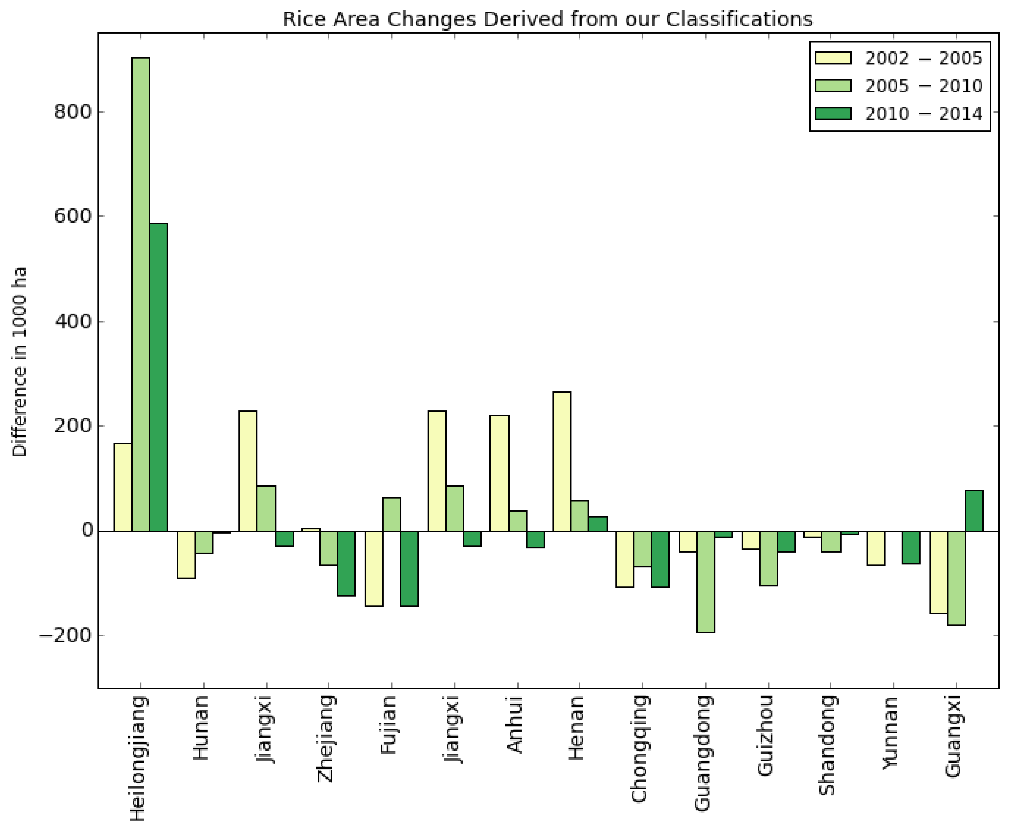
4.4. Rice Area Change

In addition to the accuracy assessment, the extracted rice areas from our classifications for each province and the years 2002, 2005, 2010 and 2014 were used to quantify rice area changes. For each province, we compared the classified rice area to the previous classification and calculated the percentage of change (Table 3).
Our classifications show that the paddy rice area for continental China constantly exceeded 20,000 kha. Paddy rice area in 2002 was 20,394.56 kha and increased by 865 kha to 21,259.20 kha in 2005. From 2005–2010, the rice area was reduced by 593 kha to 20,666.55 kha. The year 2014 had the largest rice area of our study period with 21,536.33 kha, an increase of 870 kha compared to 2010 and 1142 kha when compared to the rice area of 2002. From 2002, through 2005 and 2010, and to 2014, the change in rice area for continental China never exceeded 5% from one classification to the other.
While the overall paddy rice area remained largely stable, we can observe shifts in rice area of the provinces (Figure 7). The northernmost province, Heilongjiang, saw a rice area increase of 183% from 2002–2014. It is now the province with the largest paddy rice area and number three in terms of rice production after Hunan, whose rice area decreased every year, and Jiangxi, which saw an increase from 2002–2010, followed by a slight decrease to 2014. This increase of paddy rice area in the north came at the expense of rice area decrease in the southern provinces. Zhejiang and Fujian saw a reduction in rice area by 28% and 58%, respectively, from 2002–2014. Jiangxi, Anhui and Henan, on the other hand, had net rice area increases of 20%, 14% and 81%, albeit with some area losses for the first two, from 2010–2014. Chongqing, Guangdong, Guizhou, Shandong and Yunnan experienced constant losses in rice area for every year we classified. Guangxi showed large losses in rice area from 2002–2010 with a notable increase from 2010–2014. Our results show that most provinces in China’s south experienced a net loss in paddy rice area, with the coastal provinces showing the clearest trend, whereas the southeastern provinces that are further inland exhibited a more diverse behavior in regard to changes in their paddy rice areas.
Within the provinces, changes in paddy rice area are far from being uniformly distributed. Our classifications show where paddy area was gained and lost. Three example regions that saw substantial shifts are shown in Figure 8.
Figure 8a shows the increase of paddy rice area at the river bifurcation of the Heilong Jiang and Songhua Jiang rivers in Heilongjiang province. The rice areas from 2002–2005 show no significant change. From 2005–2010, we can observe an increase in paddy rice area and even further from 2010–2014. By 2014, the largest part of the agricultural area between the two rivers is dedicated to rice. Overall, Heilongjiang province saw a massive increase in grain production and is now China’s largest grain producer, contributing upwards of 10% to the countries rice production [2]. Figure 8b shows the decreasing rice areas in the coastal provinces with the example of Dongshan Bay, Fujian province. From 2002–2005, our classifications indicate a loss in rice area followed by almost complete depletion towards 2010. By 2014, only small patches along the river plains further from the coast are still classified as rice. We suspect that this might be due to rice paddies being converted to other crops and possibly conversion to aquaculture ponds, since the southeast coast of China is the World’s leading aquaculture region [72]. Figure 8c shows the plain at Beimin Lake in Hunan province, which was dominated by rice agriculture in 2002 and saw a constant decrease on overall paddy rice area throughout the years we studied. The most visible decrease can be seen in the southwest, south of Guanting Reservoir, where in 2010, almost none of the rice area from 2002 is cultivated anymore. The same holds true for the western and northwestern part, between Wangjiachang and Weishui Reservoir, where the rice area diminished prominently after 2005.

5. Discussion

A novel rice mapping approach using hyper-temporal MODIS data and a one-class support vector machine was developed and applied to continental China. Our results show that the overall paddy rice area remained largely stable between 2002 and 2014, which is in line with previous studies [23,31,34,53] and the agricultural census data published by the National Bureau of Statistics of China. Our maps are able to show detailed shifts in rice area on the local to county scale, which could not be deduced from the publicly-available agricultural statistics. The biggest observable change during the time period studied is the large increase in rice area in Heilongjiang, which has also been reported by previous studies [36,38,40,42]. From 2005 onward, paddy rice area in Heilongjiang increased at an unprecedented rate. We suspect that this behavior is largely driven by China’s increasing demand for rice as a food supply and the compensation of cropland loss in southern China by cropland gains in the north [73]. The increase of paddy rice area and agriculturally-used land is also made possible by rising temperatures, as well as an increase of irrigated areas by means of newly-constructed pump wells and irrigation channels [42,74]. In 2014, China was the largest producer of rice and a large importer of internationally-traded rice. Since the rice yield per sown area cannot be increased indefinitely and paddy area density lessened in the southern provinces [34], we suspect this increase in area dedicated to rice agriculture will continue in China’s northeastern provinces to satisfy the rice demand and compensate for area losses in the southern provinces.
We used MODIS data in our method, which have been preprocessed from the raw data into composites with vegetation indices and quality flags included. We chose the MOD13Q1 and MYD13Q1 datasets because their advantages and limitations are well studied and reported; they are continuously improved and are freely available, as well as easy to use for anyone who wants to replicate our approach or transfer it to other rice growing regions. By extracting features that are robust to temporal overlap and the length of the time series, we were able to incorporate the year 2002 in our classification approach. 2002 has less data points than the other years due to the Aqua satellite, from which the MYD13Q1 are derived, being launched in May 2002.
Based on the features extracted from the MODIS time series, we classified rice areas with a one-class support vector machine. We chose this classifier for two main reasons: it is not influenced by uneven class distribution, and it works well with a limited amount of training data. Classifying paddy rice areas in a study region as large as China is an inherently imbalanced classification task. Rice is China’s second largest crop after corn, according to Sown Area [2]. Even though rice paddies make up a large part of the arable land, they only make up a small fraction of China’s total land cover. Support vector machines provide a classification framework that works well in cases of such uneven class distribution. Employing a ‘one-against-all’ binary classification of rice and no_rice would have been a daunting endeavor, since it would require the collection of training data for all possible land cover in China that is not rice. Our OCSVM model obviates the need for training samples from the outlier class and was trained only with samples from our target class: rice. The model was solely trained with samples from the year 2014, and the results of our accuracy assessment show that it can be used to predict rice areas from other years, as well.
The accuracy assessment of our classifications show an overall accuracy of 0.90 when compared to our 2014 reference polygons, 0.64 compared to the AMS points and coefficients of determination larger than 0.90 compared to the official agriculture statistics. The comparison to data from China’s Statistical Yearbooks on the province level has the limitation that the area measured by our classification and the sown areas published are not directly comparable. In the statistics, the Sown Area per Season is published, and from that, it is not possible to deduce the total area of paddies with at least one rice crop per year, which is what our classification method measured. A direct comparison is only possible in provinces where only one rice season is cultivated, which resulted in R2 of 0.780, 0.820 and 0.911 for 2002, 2005 and 2010, respectively. Comparison of our results to the Sown Area with the largest extent yielded higher R2, but likely included uncertainties due to underestimation of the total area of paddies due to the effects of multi-cropping. In Sichuan, and to some extent in other provinces, our classification shows a paddy area increase by 30% followed by a 30% decrease from 2002, through 2005–2010, which is not in line with the published Sown Areas. We suspect that these fluctuations are, on the one hand, caused by the hilly terrain present in Sichuan and other southern (southwestern) provinces, which increases omission and commission errors due to mixed pixels. On the other hand, we are also not able to rule out that this error is partly caused by our classification process. We trained the model with reference data from a single year and classified multiple years with it. It is possible that in Sichuan, our model overestimated rice area for 2005 or underestimated it for 2002 and 2010. For most regions and years, we could not identify a systematic over- or under-estimation of paddy area. In the northeastern provinces, Heilongjiang, Liaoning and Jilin, the comparison showed that our classification constantly underestimates rice area in these regions. We were not able to find a systematic error in our classification approach that causes this, but suspect it might be caused by the rice cropping schemes employed in these regions.
A comparison of sown areas of rice also includes errors introduced by mixed pixel effects inherent in moderate resolution satellite images. Most rice paddies are smaller than the 250-m pixel size of our MODIS data, and as such, a pixel classified as rice also contains no_rice land cover, such as streets, buildings, trees, ponds and other small-scale agriculture. The inverse is also true in that a pixel classified as no_rice can contain small rice paddies that are undetected by our classification. The error introduced by mixed pixel effects is highly dependent on the uniformity of the land cover [26,27,35] and, therefore, varies by region. Uniform, large paddy field areas in Heilongjiang likely have little commission errors, while rice terraces in the hilly regions of south China will introduce a commission error in the classification. Recent advances in rice mapping at 30-m spatial resolution using the Landsat archives might enable future studies using MODIS data to quantify the error introduced by mixed pixels. Our reference datasets do not allow for a quantization of the error introduced by the mixed pixel effect, but the agreement with the published Sown Areas indicates that the omission and commission errors introduced by mixed pixels cancel each other out.
In the provinces of south China, errors are likely introduced by the hilly terrain and rice terraces. The resolution of MODIS data limits the ability of our approach to accurately map these small-scale paddy field terraces. The good area agreement between our classification and the statistical data suggests that these sources of uncertainty cancel each other out. Regarding the comparison of AMS points and OCSVM2002, uncertainties are introduced by the different mapping units. Our point data refer to the location of a single station within a rice field and contain no metadata about the exact location inside the field and the field size. Errors might therefore be introduced by AMS points in very small rice paddies, which cannot be detected with MODIS data, as well as mixed pixels when the station was located at a field’s edge.

6. Conclusions

Our study presents a novel rice mapping product for the years 2002, 2005, 2010 and 2014 at higher resolution than currently available maps for continental China. In our approach, we trained a one-class support vector machine with training data from the year 2014 and employed it to map rice paddies based on MODIS time series data. We extracted time series features that are robust in regards to data gaps induced by frequent cloud cover, as well as possible temporal overlaps in our synthetic eight-day time series. Our classification has an overall accuracy of 0.90 and a kappa coefficient of 0.77, compared to the 2014 reference dataset. Our results correlate highly with sown area data from the agricultural census at the province level, with R2 ranging from 0.90–0.93. Our approach should be transferable to other sensors that deliver dense time series with medium to low spatial resolution over paddy rice areas, such as MERIS or the recently-launched Sentinel-3.
With our study, we aim to fill a gap in the currently available rice mapping products for China that are either spatially or temporally limited or at a coarser resolution. The delivery of such products in a timely and accurate manner is important for decision makers in the context of food security and international rice trade. Knowledge about the location and extent of paddy rice areas is also valuable for the Earth systems and hydrological modelling scientific community, as rice is a large consumer of water and a producer of green-house-relevant methane emissions. In a time of ever-increasing amounts of openly available high resolution satellite data from missions, like Copernicus Sentinel-1, Sentinel-2 and Landsat-8, medium resolution rice maps are useful for the remote sensing community to reduce the amount of data and processing time necessary for creating high resolution rice maps.

Acknowledgments

This research has been partially funded by the German Ministry of Education and Science (BMBF) in the context of the DELIGHT project, as well as the National Natural Science Foundation of China with Grant No. 41430861.

Author Contributions

K.C. and C.K. designed the research concept. K.C. processed and analyzed the data. H.Y. shared the AMS reference data and helped with the accuracy assessment. All authors jointly discussed the results. K.C. authored the first version of the manuscript, and C.K. and H.Y. commented and worked on the manuscript.

Conflicts of Interest

The authors declare no conflict of interest.

Abbreviations

The following abbreviations are used in this manuscript:
AMSAgricultural Meteorological Station
EVIEnhanced Vegetation Index
LSWILand Surface Water Index
MIRMid-Infrared
MODISModerate Resolution Imaging Spectroradiometer
NDVINormalized Difference Vegetation Index
NIRNear-Infrared
OCSVMOne-Class Support Vector Machine
RBFRadial Basis Function
SPOT-VGTSatellite Pour l’Observation de la Terre-Vegetation
SVMSupport Vector Machine
TSTime Series

Appendix A

Software packages used for reading the spatial data, processing it, training the OCSVM model and predicting paddy rice areas:
  • Python 2.7.9 [75]
  • GDAL 1.11.2 [76]
  • numpy 1.10.0 [77]
  • scikit-learn 0.16.1 [78]
  • pandas 0.16.2 [79]
  • scipy 0.16.0 [80]

References

  1. FAOSTAT Paddy Rice Production and Trade 2014. Available online: http://faostat3.fao.org (accessed on 3 February 2016).
  2. National Bureau of Statistics of China. China Statistical Yearbook 2014; China Statistics Press: Beijing, China, 2014.
  3. De Datta, S. Principles and Practices of Rice Production; Wiley: New York, NY, USA, 1981. [Google Scholar]
  4. Kuenzer, C.; Knauer, K. Remote sensing of rice crop areas. Int. J. Remote Sens. 2013, 34, 2101–2139. [Google Scholar] [CrossRef]
  5. Mosleh, M.K.; Hassan, Q.K.; Chowdhury, E.H. Application of remote sensors in mapping rice area and forecasting its production: A review. Sensors 2015, 15, 769–791. [Google Scholar] [CrossRef] [PubMed]
  6. Bouvet, A.; Le Toan, T. Use of ENVISAT/ASAR wide-swath data for timely rice fields mapping in the Mekong River Delta. Remote Sens. Environ. 2011, 115, 1090–1101. [Google Scholar] [CrossRef] [Green Version]
  7. Ribbes, F.; Le Toan, T. Rice field mapping and monitoring with RADARSAT data. Int. J. Remote Sens. 1999, 20, 745–765. [Google Scholar] [CrossRef]
  8. Le Toan, T.; Ribbes, F.; Floury, N.; Fujita, M.; Kurosu, T.; Wang, L.F.; Floury, N.; Ding, K.H.; Kong, J.A.; Fujita, M.; et al. Rice crop mapping and monitoring using ERS-1 data based on experiment and modeling results. IEEE Trans. Geosci. Remote Sens. 1997, 35, 41–56. [Google Scholar] [CrossRef]
  9. Lam-Dao, N.; Le Toan, T.; Apan, A.; Bouvet, A.; Young, F.; Le-Van, T. Effects of changing rice cultural practices on C-band synthetic aperture radar backscatter using Envisat advanced synthetic aperture radar data in the Mekong River Delta. J. Appl. Remote Sens. 2009, 3, 033563. [Google Scholar] [Green Version]
  10. Inoue, Y.; Kurosu, T.; Maeno, H.; Uratsuka, S.; Kozu, T.; Dabrowska-Zielinska, K.; Qi, J. Season-long daily measurements of multifrequency (Ka, Ku, X, C, and L) and full-polarization backscatter signatures over paddy rice field and their relationship with biological variables. Remote Sens. Environ. 2002, 81, 194–204. [Google Scholar] [CrossRef]
  11. Nguyen, D.; Clauss, K.; Cao, S.; Naeimi, V.; Kuenzer, C.; Wagner, W. Mapping rice seasonality in the Mekong Delta with multi-year Envisat ASAR WSM data. Remote Sens. 2015, 7, 15868–15893. [Google Scholar] [CrossRef]
  12. Nelson, A.; Setiyono, T.; Rala, A.; Quicho, E.; Raviz, J.; Abonete, P.; Maunahan, A.; Garcia, C.; Bhatti, H.; Villano, L.; et al. Towards an operational SAR-based rice monitoring system in Asia: Examples from 13 demonstration sites across Asia in the RIICE Project. Remote Sens. 2014, 6, 10773–10812. [Google Scholar] [CrossRef]
  13. Xiao, X.; Boles, S.; Frolking, S.; Li, C.; Babu, J.Y.; Salas, W.; Moore, B. Mapping paddy rice agriculture in South and Southeast Asia using multi-temporal MODIS images. Remote Sens. Environ. 2006, 100, 95–113. [Google Scholar] [CrossRef]
  14. Gumma, M.K.; Nelson, A.; Thenkabail, P.S.; Singh, A.N. Mapping rice areas of South Asia using MODIS multitemporal data. J. Appl. Remote Sens. 2011, 5, 053547. [Google Scholar] [CrossRef]
  15. Manjunath, K.R.; More, R.S.; Jain, N.K.; Panigrahy, S.; Parihar, J.S. Mapping of rice-cropping pattern and cultural type using remote-sensing and ancillary data: A case study for South and Southeast Asian countries. Int. J. Remote Sens. 2015, 36, 6008–6030. [Google Scholar] [CrossRef]
  16. Motohka, T.; Nasahara, K.N.; Miyata, A.; Mano, M.; Tsuchida, S. Evaluation of optical satellite remote sensing for rice paddy phenology in monsoon Asia using a continuous in situ dataset. Int. J. Remote Sens. 2009, 30, 4343–4357. [Google Scholar] [CrossRef]
  17. Nguyen, T.T.H.; De Bie, C.A.J.M.; Ali, A.; Smaling, E.M.A.; Chu, T.H. Mapping the irrigated rice cropping patterns of the Mekong delta, Vietnam, through hyper-temporal SPOT NDVI image analysis. Int. J. Remote Sens. 2012, 33, 415–434. [Google Scholar] [CrossRef]
  18. Peng, D.; Huete, A.R.; Huang, J.; Wang, F.; Sun, H. Detection and estimation of mixed paddy rice cropping patterns with MODIS data. Int. J. Appl. Earth Obs. Geoinf. 2011, 13, 13–23. [Google Scholar] [CrossRef]
  19. Boschetti, M.; Nutini, F.; Manfron, G.; Brivio, P.A.; Nelson, A. Comparative analysis of normalised difference spectral indices derived from MODIS for detecting surface water in flooded rice cropping systems. PLoS ONE 2014, 9. [Google Scholar] [CrossRef] [PubMed]
  20. Boschetti, M.; Nelson, A.; Nutini, F.; Manfron, G.; Busetto, L.; Barbieri, M.; Laborte, A.; Raviz, J.; Holecz, F.; Mabalay, M.; et al. Rapid assessment of crop status: An application of MODIS and SAR data to rice areas in Leyte, Philippines affected by Typhoon Haiyan. Remote Sens. 2015, 7, 6535–6557. [Google Scholar] [CrossRef]
  21. Asilo, S.; de Bie, K.; Skidmore, A.; Nelson, A.; Barbieri, M.; Maunahan, A. Complementarity of two rice mapping approaches: Characterizing strata mapped by hypertemporal MODIS and rice paddy identification using multitemporal SAR. Remote Sens. 2014, 6, 12789–12814. [Google Scholar] [CrossRef]
  22. Wang, J.; Xiao, X.; Qin, Y.; Dong, J.; Zhang, G.; Kou, W.; Jin, C.; Zhou, Y.; Zhang, Y. Mapping paddy rice planting area in wheat-rice double-cropped areas through integration of Landsat-8 OLI, MODIS, and PALSAR images. Sci. Rep. 2015, 5, 1–11. [Google Scholar] [CrossRef] [PubMed]
  23. Xiao, X.; Boles, S.; Liu, J.; Zhuang, D.; Frolking, S.; Li, C.; Salas, W.; Moore, B. Mapping paddy rice agriculture in southern China using multi-temporal MODIS images. Remote Sens. Environ. 2005, 95, 480–492. [Google Scholar] [CrossRef]
  24. Xiao, X.; Boles, S.; Frolking, S.; Salas, W.; Moore, B.; Li, C.; He, L.; Zhao, R. Observation of flooding and rice transplanting of paddy rice fields at the site to landscape scales in China using VEGETATION sensor data. Int. J. Remote Sens. 2002, 23, 3009–3022. [Google Scholar] [CrossRef]
  25. Sakamoto, T.; Yokozawa, M.; Toritani, H.; Shibayama, M.; Ishitsuka, N.; Ohno, H. A crop phenology detection method using time-series MODIS data. Remote Sens. Environ. 2005, 96, 366–374. [Google Scholar] [CrossRef]
  26. Sakamoto, T.; Van Nguyen, N.; Ohno, H.; Ishitsuka, N.; Yokozawa, M. Spatio-temporal distribution of rice phenology and cropping systems in the Mekong Delta with special reference to the seasonal water flow of the Mekong and Bassac rivers. Remote Sens. Environ. 2006, 100, 1–16. [Google Scholar] [CrossRef]
  27. Son, N.T.; Chen, C.F.; Chen, C.R.; Duc, H.N.; Chang, L.Y. A phenology-based classification of time-series MODIS data for rice crop monitoring in Mekong Delta, Vietnam. Remote Sens. 2014, 6, 135–156. [Google Scholar] [CrossRef]
  28. Chen, C.F.; Son, N.T.; Chang, L.Y.; Chen, C.R. Classification of rice cropping systems by empirical mode decomposition and linear mixture model for time-series MODIS 250 m NDVI data in the Mekong Delta, Vietnam. Int. J. Remote Sens. 2011, 32, 5115–5134. [Google Scholar] [CrossRef]
  29. Guan, X.; Huang, C.; Liu, G.; Meng, X.; Liu, Q. Mapping rice cropping systems in Vietnam using an NDVI-based time-series similarity measurement based on DTW distance. Remote Sens. 2016, 8, 1–25. [Google Scholar] [CrossRef]
  30. Chen, C.-F.; Son, N.-T.; Chen, C.-R.; Cho, K.; Hsiao, Y.-Y.; Chiang, S.-H.; Chang, L.-Y. Assessing rice crop damage and restoration using remote sensing in tsunami-affected areas, Japan. J. Appl. Remote Sens. 2015, 9, 096002–1–096002–19. [Google Scholar] [CrossRef]
  31. Frolking, S.; Qiu, J.; Boles, S.; Xiao, X.; Liu, J.; Zhuang, Y.; Li, C.; Qin, X. Combining remote sensing and ground census data to develop new maps of the distribution of rice agriculture in China. Glob. Biogeochem. Cycles 2002, 16, 38:1–38:10. [Google Scholar] [CrossRef]
  32. Sun, H.; Huang, J.; Huete, A.R.; Peng, D.; Zhang, F. Mapping paddy rice with multi-date moderate-resolution imaging spectroradiometer (MODIS) data in China. J. Zhejiang Univ. Sci. A 2009, 10, 1509–1522. [Google Scholar] [CrossRef]
  33. Qiu, B.; Li, W.; Tang, Z.; Chen, C.; Qi, W. Mapping paddy rice areas based on vegetation phenology and surface moisture conditions. Ecol. Indic. 2015, 56, 79–86. [Google Scholar] [CrossRef]
  34. Qiu, B.; Qi, W.; Tang, Z.; Chen, C.; Wang, X. Rice cropping density and intensity lessened in southeast China during the twenty-first century. Environ. Monit. Assess. 2016, 188, 1–12. [Google Scholar] [CrossRef] [PubMed]
  35. Shi, J.; Huang, J. Monitoring spatio-temporal distribution of rice planting area in the Yangtze River Delta region using MODIS images. Remote Sens. 2015, 7, 8883–8905. [Google Scholar] [CrossRef]
  36. Jin, C.; Xiao, X.; Dong, J.; Qin, Y.; Wang, Z. Mapping paddy rice distribution using multi-temporal Landsat imagery in the Sanjiang Plain, northeast China. Front. Earth Sci. 2016, 10, 49–62. [Google Scholar] [CrossRef]
  37. Wang, J.; Huang, J.; Zhang, K.; Li, X.; She, B.; Wei, C.; Gao, J.; Song, X. Rice fields mapping in fragmented area using multi-temporal HJ-1A/B CCD images. Remote Sens. 2015, 7, 3467–3488. [Google Scholar] [CrossRef]
  38. Shi, J.; Huang, J.; Zhang, F. Multi-year monitoring of paddy rice planting area in Northeast China using MODIS time series data. J. Zhejiang Univ. Sci. B 2013, 14, 934–946. [Google Scholar] [CrossRef] [PubMed]
  39. Zhou, Y.; Xiao, X.; Qin, Y.; Dong, J.; Zhang, G.; Kou, W.; Jin, C.; Wang, J.; Li, X. Mapping paddy rice planting area in rice-wetland coexistent areas through analysis of Landsat 8 OLI and MODIS images. Int. J. Appl. Earth Obs. Geoinf. 2016, 46, 1–12. [Google Scholar] [CrossRef]
  40. Zhao, Q.; Lenz-Wiedemann, V.; Yuan, F.; Jiang, R.; Miao, Y.; Zhang, F.; Bareth, G. Investigating within-field variability of rice from high resolution satellite imagery in Qixing Farm County, Northeast China. ISPRS Int. J. Geo-Inf. 2015, 4, 236–261. [Google Scholar] [CrossRef]
  41. Kontgis, C.; Schneider, A.; Ozdogan, M. Mapping rice paddy extent and intensification in the Vietnamese Mekong River Delta with dense time stacks of Landsat data. Remote Sens. Environ. 2015, 169, 255–269. [Google Scholar] [CrossRef]
  42. Dong, J.; Xiao, X.; Kou, W.; Qin, Y.; Zhang, G.; Li, L.; Jin, C.; Zhou, Y.; Wang, J.; Biradar, C.; Liu, J.; Moore, B. Tracking the dynamics of paddy rice planting area in 1986–2010 through time series Landsat images and phenology-based algorithms. Remote Sens. Environ. 2015, 160, 99–113. [Google Scholar] [CrossRef]
  43. Dong, J.; Xiao, X.; Menarguez, M.A.; Zhang, G.; Qin, Y.; Thau, D.; Biradar, C.; Moore, B. Mapping paddy rice planting area in northeastern Asia with Landsat 8 images, phenology-based algorithm and Google Earth Engine. Remote Sens. Environ. 2016. [Google Scholar] [CrossRef]
  44. He, H.; Garcia, E.A. Learning from imbalanced data. IEEE Trans. Knowl. Data Eng. 2009, 21, 1263–1284. [Google Scholar]
  45. Mountrakis, G.; Im, J.; Ogole, C. Support vector machines in remote sensing: A review. ISPRS J. Photogramm. Remote Sens. 2011, 66, 247–259. [Google Scholar] [CrossRef]
  46. Tax, D.M.J.; Duin, R.P.W. Support vector data description. Mach. Learn. 2004, 54, 45–66. [Google Scholar] [CrossRef]
  47. Liu, B.; Dai, Y.; Li, X.; Lee, W.S.; Yu, P.S. Building text classifiers using positive and unlabeled examples. In Proceedings of the Third IEEE International Conference on Data Mining, Melbourne, FL, USA, 19–22 November 2003; pp. 179–186.
  48. Schölkopf, B.; Williamson, R.C.; Smola, A.J.; Shawe-Taylor, J.; Platt, J.C. Support Vector Method for Novelty Detection. In 13th Annual Neural Information Processing Systems Conference (NIPS 1999); Solla, S.A., Leen, T.K., Müller, K.-R., Eds.; MIT Press: Denver, CO, USA, 2000; pp. 582–588. [Google Scholar]
  49. Schölkopf, B.; Platt, J.C.; Shawe-Taylor, J.; Smola, A.J.; Williamson, R.C. Estimating the support of a high-dimensional distribution. Neural Comput. 2001, 13, 1443–1471. [Google Scholar] [CrossRef] [PubMed]
  50. National Bureau of Statistics of China. China Statistical Yearbook 2002; China Statistics Press: Beijing, China, 2002.
  51. National Bureau of Statistics of China. China Statistical Yearbook 2005; China Statistics Press: Beijing, China, 2005.
  52. National Bureau of Statistics of China. China Statistical Yearbook 2010; China Statistics Press: Beijing, China, 2010.
  53. Li, L.; Friedl, M.; Xin, Q.; Gray, J.; Pan, Y.; Frolking, S. Mapping crop cycles in China using MODIS-EVI time series. Remote Sens. 2014, 6, 2473–2493. [Google Scholar] [CrossRef]
  54. Zhao, D.; Kuenzer, C.; Fu, C.; Wagner, W. Evaluation of the ERS scatterometer-derived soil water index to monitor water availability and precipitation distribution at three different scales in China. J. Hydrometeorol. 2008, 9, 549–562. [Google Scholar] [CrossRef]
  55. Didan, K. MOD13Q1 MODIS/Terra Vegetation Indices 16-Day L3 Global 250 m SIN Grid V006; NASA EOSDIS Land Processes DAAC; NASA: College Park, MD, USA, 2015.
  56. Didan, K. MYD13Q1 MODIS/Aqua Vegetation Indices 16-Day L3 Global 250 m SIN Grid V006; NASA EOSDIS Land Processes DAAC; NASA: College Park, MD, USA, 2015.
  57. Huete, A.R.; Justice, C.; van Leeuven, W. MODIS Vegetation Index (MOD13) Algorithm Theoretical Basis Document (ATBD) Version 3; University of Arizona: Tucson, AZ, USA, 1999. [Google Scholar]
  58. Vermote, E.F.; El Saleous, N.Z.; Justice, C.O. Atmospheric correction of MODIS data in the visible to middle infrared: First results. Remote Sens. Environ. 2002, 83, 97–111. [Google Scholar] [CrossRef]
  59. Vermote, E.F.; Kotchenova, S. Atmospheric correction for the monitoring of land surfaces. J. Geophys. Res. 2008, 113, 1–12. [Google Scholar] [CrossRef]
  60. Vermote, E.F.; Vermeulen, A. Athmospheric Correction Algorithm: Spectral Reflectances (MOD09), MODIS Algorithm Theoretical Basis Document Version 4; NASA: College Park, MD, USA, 1999.
  61. Land Processes Distributed Active Archiving Center Data Pool. Available online: http://e4ftl01.cr.usgs.gov/ (accessed on 1 June 2015).
  62. Chen, J.; Jönsson, P.; Tamura, M.; Gu, Z.; Matsushita, B.; Eklundh, L. A simple method for reconstructing a high-quality NDVI time-series data set based on the Savitzky-Golay filter. Remote Sens. Environ. 2004, 91, 332–344. [Google Scholar] [CrossRef]
  63. Yan, H.; Xiao, X.; Huang, H.; Liu, J.; Chen, J.; Bai, X. Multiple cropping intensity in China derived from agro-meteorological observations and MODIS data. Chin. Geogr. Sci. 2014, 24, 205–219. [Google Scholar] [CrossRef]
  64. Hastie, T.; Tibshirani, R.; Friedman, J. The Elements of Statistical Learning; Springer Series in Statistics; Springer New York: New York, NY, USA, 2009. [Google Scholar]
  65. Hijmans, R.; Kapoor, J.; Wieczorek, J.; Garcia, N.; Maunahan, A.; Rala, A.; Mandel, A. Global Administrative Areas, Version 2.0. Available online: http://www.gadm.org/ (accessed on 1 May 2015).
  66. Baldeck, C.A.; Asner, G.P. Single-species detection with airborne imaging spectroscopy data: A comparison of support vector techniques. IEEE J. Sel. Top. Appl. Earth Obs. Remote Sens. 2015, 8, 2501–2512. [Google Scholar] [CrossRef]
  67. Drake, J.M.; Randin, C.; Guisan, A. Modelling ecological niches with support vector machines. J. Appl. Ecol. 2006, 43, 424–432. [Google Scholar] [CrossRef]
  68. Baldi, P.; Brunak, S.; Chauvin, Y.; Andersen, C.A.F.; Nielsen, H. Assessing the accuracy of prediction algorithms for classification: an overview. Bioinformatics 2000, 16, 412–424. [Google Scholar] [CrossRef] [PubMed]
  69. Olofsson, P.; Foody, G.M.; Herold, M.; Stehman, S.V.; Woodcock, C.E.; Wulder, M.A. Good practices for estimating area and assessing accuracy of land change. Remote Sens. Environ. 2014, 148, 42–57. [Google Scholar] [CrossRef]
  70. Powers, D. Evaluation: From precision, recall and f-measure to roc., informedness, markedness & correlation. J. Mach. Learn. Technol. 2011, 2, 37–63. [Google Scholar]
  71. Cohen, J. A Coefficient of Agreement for Nominal Scales. Educ. Psychol. Meas. 1960, 20, 37–46. [Google Scholar] [CrossRef]
  72. Ottinger, M.; Clauss, K.; Kuenzer, C. Aquaculture: Relevance, distribution, impacts and spatial assessments—A review. Ocean Coast. Manag. 2016, 119, 244–266. [Google Scholar] [CrossRef]
  73. Liu, J.; Kuang, W.; Zhang, Z.; Xu, X.; Qin, Y.; Ning, J.; Zhou, W.; Zhang, S.; Li, R.; Yan, C.; et al. Spatiotemporal characteristics, patterns, and causes of land-use changes in China since the late 1980s. J. Geogr. Sci. 2014, 24, 195–210. [Google Scholar] [CrossRef]
  74. Okamoto, K.; Kawashima, H. Estimating total area of paddy fields in Heilongjiang, China, around 2000 using Landsat Thematic Mapper/Enhanced Thematic Mapper Plus data. Remote Sens. Lett. 2016, 7, 533–540. [Google Scholar] [CrossRef]
  75. Python Software Foundation Python 2.7.9. Available online: https://www.python.org/downloads/release/python-279/ (accessed on 12 May 2015).
  76. Open Source Geospatial Foundation. GDAL—Geospatial Data Abstraction Library, Version 1.11; Available online: http://gdal.osgeo.org (accessed on 1 February 2015).
  77. Van der Walt, S.; Colbert, S.C.; Varoquaux, G. The NumPy Array: A structure for efficient numerical computation. Comput. Sci. Eng. 2011, 13, 22–30. [Google Scholar] [CrossRef]
  78. Pedregosa, F.; Varoquaux, G.; Gramfort, A.; Michel, V.; Thirion, B.; Grisel, O.; Blondel, M.; Prettenhofer, P.; Weiss, R.; Dubourg, V.; et al. Scikit-learn: Machine Learning in Python. J. Mach. Learn. Res. 2011, 12, 2825–2830. [Google Scholar]
  79. McKinney, W. Data Structures for Statistical Computing in Python. In Proceedings of the 9th Python in Science Conference, Austin, TX, USA, 28 June–3 July 2010; pp. 51–56.
  80. Jones, E.; Oliphant, T.; Peterson, P. SciPy: Open Source Scientific Tools for Python, Version: 0.16.0; Available online: http://www.scipy.org/ (accessed on 2 June 2015).
Figure 1. Rice production in mainland China 2014. Based on data from [2].
Remotesensing 08 00434 g001
Figure 2. Distribution of reference data in mainland China’s major rice growing regions.
Remotesensing 08 00434 g002
Figure 3. Temporal profile of TSEVI and TSLSWI2130 of two rice paddies ((a) Lake Xingkai, Heilongjiang province; (b) Lu’an, Anhui province), a corn field ((c) Bohai Bay, Tianin province) and aquaculture ponds ((d) Dongting Lake, Hunan province).
Remotesensing 08 00434 g003
Figure 4. Results of the parameter grid search. (a) The f1-scores for all ν and ɣ combinations from the grid search; (b) a subset of ν and ɣ combinations around the one with the highest overall f1-score.
Remotesensing 08 00434 g004
Figure 5. Paddy rice classifications for mainland China.
Remotesensing 08 00434 g005
Figure 6. R2 for OCSVM2010, OCSVM2005 and OCSVM2002 compared to Sown Area of rice for the season with the largest extent (a) and Total Sown Area for provinces with one dominant rice crop per year (b).
Remotesensing 08 00434 g006aRemotesensing 08 00434 g006b
Figure 7. Provincial rice area changes from 2002–2014.
Remotesensing 08 00434 g007
Figure 8. Rice area changes in (a) Heilong Jiang Plain, Heilongjiang province, (b) Dongshan Bay, Fujian province, and (c) Beimin Lake, Hunan province. Landsat 8 RGB overview images are presented in the first row; the next four rows are based on the OCSVM classification, with slope relief derived from the Shuttle Radar Topography Mission (SRTM, 1 arc-second) Digital Elevation Modelas the background. Red stars show bifurcations of the Heilong Jiang (1) and Songhua Jiang (2) rivers, the plain at Beimin Lake (3), the southern part of Guanting Reservoir (4) and Wangjiachang Reservoir (5).
Remotesensing 08 00434 g008
Table 1. Features extracted from the MODIS time series.
FeatureInput Time Series
10th percentileTSEVI 1, TSred 2, TSNIR 3, TSblue 4, TSMIR 5, TSLSWI2130 6
25th percentileTSEVI, TSred, TSNIR, TSblue, TSMIR, TSLSWI2130
50th percentile/medianTSEVI, TSred, TSNIR, TSblue, TSMIR, TSLSWI2130
75th percentileTSEVI, TSred, TSNIR, TSblue, TSMIR, TSLSWI2130
90th percentileTSEVI, TSred, TSNIR, TSblue, TSMIR, TSLSWI2130
amplitudeTSNDVI 7, TSEVI, TSred, TSNIR, TSblue, TSMIR, TSLSWI2130
difference 75th and 25th percentileTSEVI, TSred, TSNIR, TSblue, TSMIR, TSLSWI2130
difference 90th and 10th percentileTSEVI, TSred, TSNIR, TSblue, TSMIR, TSLSWI2130
amount of local maxima >0.8TSEVI, TSLSWI2130
amount of local maxima >0.7TSEVI, TSLSWI2130
amount of local maxima >0.6TSEVI, TSLSWI2130
amount of local minima <0.4TSEVI, TSLSWI2130
amount of local minima <0.3TSEVI, TSLSWI2130
amount of local minima <0.2TSEVI, TSLSWI2130
amount of local minima <0.1TSEVI, TSLSWI2130
amount of EVI and LSWI2130 inversionsTSEVI, TSLSWI2130
1 One-year EVI time series (Layer 2), 2 1-year red (620–670 nm) time series (Layer 4), 3 1-year NIR (841–875 nm) time series (Layer 5), 4 1-year blue (459–479 nm) time series (Layer 6), 5 1-year MIR (2105–2155 nm) time series (Layer 7), 6 1-year LSWI (calculated from NIR and MIR) time series, 7 1-year NDVI time series (Layer 1).
Table 2. Confusion matrix for OCSVM2014 compared to our reference dataset.
Predictedno_ricerice
Reference
no_rice12815653
rice14185428
Table 3. Rice area and change per province in 1000 ha derived from our classifications.
OCSVM2002OCSVM2005OCSVM2010OCSVM2014
Anhui1661.8713.2%1880.882.0%1919.38−1.6%1888.12
Beijing0.37213.0%1.16−92.1%0.09411.8%0.47
Chongqing988.88−11.0%880.42−7.6%813.25−13.2%706.31
Fujian614.00−23.3%470.6613.6%534.67−27.1%389.77
Gansu3.5517.1%4.16−39.1%2.53−30.1%1.77
Guangdong1341.08−3.0%1301.10−14.9%1106.62−1.0%1095.24
Guangxi1327.83−11.8%1170.50−15.4%990.577.8%1068.04
Guizhou911.36−3.8%876.46−12.1%770.78−5.1%731.33
Hebei58.56157.3%150.68−75.6%36.70115.3%79.01
Heilongjiang903.2518.5%1070.4484.3%1972.5229.8%2560.05
Henan430.9261.1%694.328.4%752.343.6%779.70
Hubei1607.90−6.2%1508.793.1%1555.393.8%1614.46
Hunan1721.73−5.2%1631.84−2.6%1589.40−0.2%1586.33
Inner Mongolia31.5817.4%37.06−27.8%26.74133.3%62.38
Jiangsu2191.336.8%2340.44−15.7%1973.6821.5%2397.08
Jiangxi1411.4316.2%1640.375.3%1726.94−1.6%1698.67
Jilin405.49−10.4%363.27−21.1%286.7535.8%389.40
Liaoning381.79−0.3%380.6322.6%466.580.7%469.83
Ningxia31.6217.8%37.253.0%38.3766.7%63.98
Qinghai1.0565.1%1.7329.2%2.23−42.8%1.28
Shaanxi202.10−36.7%127.9937.3%175.79−15.0%149.40
Shandong210.33−5.5%198.75−20.1%158.83−4.5%151.70
Shanghai30.6054.2%47.19−15.3%39.9631.7%52.64
Shanxi2.9839.2%4.1579.6%7.4683.6%13.70
Sichuan1819.2630.0%2364.76−26.9%1727.512.2%1766.03
Tianjin6.96200.5%20.92−76.3%4.96207.1%15.25
Tibet1.21−9.3%1.1054.1%1.707.9%1.83
Xinjiang6.92253.0%24.445.4%25.7522.2%31.46
Yunnan1223.81−5.4%1157.71−0.1%1156.06−5.4%1093.33
Zhejiang864.800.6%870.03−7.7%803.00−15.6%677.77

