Mass Flux Solution in the Tibetan Plateau Using Mascon Modeling

Abstract

Mascon modeling is used in this paper to produce the mass flux solutions in the Tibetan Plateau. In the mascon modeling, the pseudo observations and their covariance matrices are derived from the GRACE monthly gravity field models. The sampling density of the pseudo observations is determined based on the eigenvalues of the covariance matrices. In the Tibetan Plateau, the sampling density of per 1.5° is the most appropriate among all choices. The mass flux variations from 2003 to 2014 are presented in this paper, which show large mass loss (about −15.5 Gt/year) in Tianshan, North India, and Eastern Himalaya, as well as strong positive signals (about 9 Gt/year) in the Inner Tibetan Plateau. After the glacier isostatic adjustment effects from Pau-5-AUT model are removed, the mass change rates in the Tibetan Plateau derived from CSR RL05, JPL RL05, GFZ RL05a, and Tongji-GRACE02 monthly models are −6.41 ± 4.74 Gt/year, −5.87 ± 4.88 Gt/year, −6.08 ± 4.65 Gt/year, and −11.50 ± 4.79 Gt/year, respectively, which indicate slight mass loss in this area. Our results confirm that mascon modeling is efficient in the recovery of time-variable gravity signals in the Tibetan Plateau.

1. Introduction

The GRACE (Gravity Recovery and Climate Experiment) satellites, launched on 17 March 2002, have accumulated more than 10 years of observations to recover the Earth’s gravity field in high spatial and temporal resolutions [1]. The time-variable Earth’s gravity field solutions from satellite tracking data are expressed in terms of either Stokes coefficients or mascon parameters. Due to relatively large errors in high degrees and orders of Stokes coefficients, several filter techniques, such as Gaussian filter [2,3], fan filter [4,5], and Wiener filter [6], have been developed to restrain the errors and recover the signals from the Stokes coefficients. Firstly proposed to analyze spacecraft tracking data in the 1970s, mascon modeling is established by a connection between mass variations and gravity potentials at satellite altitude [7,8,9,10,11,12,13]. The mascon parameters in terms of point masses [7,14,15], spherical caps [16] and finite surfaces of constant density [17,18,19,20,21] can be directly calculated from either the GRACE tracking data [7,16,17,18,19,20,21] or the Stokes coefficients of monthly gravity field models [14,15,22].

Muller and Sjogren proposed the mascon modeling in 1967 to recover planetary gravity field from satellite observations [7]. Forsberg and Reeh successfully applied the mascon solution in calculating the mass flux over the Greenland from the GRACE Stokes coefficients without using filtering techniques [14], which can reduce the loss of gravity signals. Baur and Sneeuw demonstrated that the mascon modeling provided reasonable ice-mass decline trend in Greenland with both GRACE Level 2 products and simulated gravitational signals [15]. However, the impacts of the covariance matrices of the gravitational disturbance calculated from the GRACE monthly solutions were not discussed before, which are helpful to determine the sampling density of the mascon parameters; and the mascon solutions in the Tibetan Plateau were not compared and discussed using the latest models (RL05 or RL05a) from different research groups, such as Center for Space Research (CSR), GeoForschungZentrum (GFZ), and Jet Propulsion Laboratory (JPL).

Located in the southwest of China, the Tibetan Plateau is known as the Third Pole for its massive storage of water in terms of lakes and glaciers [23], which also indicates that it plays an important role in global climate dynamic [24,25]. The study of mass flux in the Tibetan Plateau is always an interest topic among geoscientists due to the geographic complexity: Yi and Sun concluded a ice-mass loss of −35.0 ± 5.8 Gt/year in High Mountain Asia from 10-year GRACE monthly solutions using the Space Domain Inverse method [26]; Jacob et al. presented a GRACE-based result over Himalayas, which indicates a slight mass loss of −4 ± 20 Gt/year from January 2003 to December 2010 [27]; Song et al. estimated a rising rate of about 6.79 Gt/year in the Inner Tibetan Plateau from ICESat/GLAS altimetry data and remote sensing images [25].

In this paper, we estimate the mass flux variations in the Tibetan Plateau from 2003 to 2014 using the mascon modeling, where the covariance of pseudo observations of gravitational disturbance is derived from the covariance of the Stokes coefficients of GRACE monthly gravity field model. The rest of the paper is organized as follows. In Section 2, the mathematical model is presented to clarify how the mascon model is established, and its regularization solution. In Section 3, the mass flux in the Tibetan Plateau is presented in terms of trend and annual changes, and the spatial distribution. The results are compared with previous studies in Section 4 and the conclusions are drawn in Section 5.

2. Materials and Methodology

2.1. Research Area

The Tibet is a part of the Tibetan Plateau—a vast flat highland covering an area of around 3,617,367 km² with an altitude above 4000 m on average [23]. Located at the center of Asia, the Tibetan Plateau is surrounded by numerous glaciers and lakes [24], which make it the source of several major rivers in Asia, such as the Ganges, Indus and Yangtze. Figure 1 shows the location of the Tibetan Plateau (shown in yellow) and the research area within the black rectangular frame (64°E–108°E, 20°N–46°N), as well as major waterways over this region. The complex geographic conditions and massive water storages in the forms of glaciers, rivers, and lakes lead to huge difficulties in recovery of glacier melting rates, water seasonal variations, tectonic motions etc., which are partly attributed to poor conditions for carrying out ground-based observations, e.g., the severe weather and the oxygen-poor environment. In this paper, the mass flux variations in the Tibetan Plateau are calculated from 11-year time series of monthly gravity field models.

2.2. Data

2.2.1. GRACE Monthly Solutions

Since the launch of GRACE satellites in 2002, a series of static and time-variable gravity field models have been published for geophysical and climate researches on the ICGEM (International Center for Global Earth Models) [28]. In this paper, the GRACE monthly gravity field models, i.e., CSR RL05 [29], JPL RL05 [30], GFZ RL05a [31], and Tongji-GRACE02 (Tongji University, Shanghai, China) [32] are used. All C₂₀ terms and their uncertainties derived from the GRACE monthly solutions are replaced by those from satellite laser ranging data [33].

Table 1. The time period and the numbers of missing months of GRACE monthly solutions.

Gravity Model	Time Period	Numbers of Months without Data
CSR RL05	April 2002–October 2014	12
JPL RL05	April 2002–September 2014	12
GFZ RL05a	April 2002–August 2014	12
Tongji-GRACE02	January 2003–April 2015	11

shows the time span of the models, as well as the numbers of missing months. Therefore, nearly 12-year sequences of time-variable gravity field are used to reveal long-time tendency of the mass flux in the Tibet Plateau.

Since we are interested in the time-variable signals, a mean gravity field should be subtracted,

$$\Delta C_{lm}=C_{lm}-C_{lm}^{mean},\Delta S_{lm}=S_{lm}-S_{lm}^{mean}$$

(1)

where $C_{lm}$ and $S_{lm}$ are the Stokes coefficients of monthly gravity models; $C_{lm}^{mean}$ and $S_{lm}^{mean}$ are their mean values, $\Delta C_{lm}$ and $\Delta S_{lm}$ are the coefficients after the mean field is removed; l and m indicate the degree and order of gravity field model.

The radial gravitational disturbance can be expressed in terms of fully normalized Stokes coefficients $\Delta C_{lm}$ and $\Delta S_{lm}$ as follows [15,34],

$$\delta g=-\frac{GM}{r^2}{\displaystyle \sum _{l=1}^{l_{\max }}{(\frac{a}{r})}^l}(l+1){\displaystyle \sum _{m=0}^l{P}_{lm}(\sin \phi )(\Delta C_{lm}}\cos m\lambda +\Delta S_{lm}\sin m\lambda )$$

(2)

In Equation (2), r, $\lambda$ and $\phi$ are the spherical coordinates of the computed point, i.e., the radius, longitude, and the latitude, respectively; GM indicates the gravitational constant; a is the mean radius of the Earth; P_lm stands for the fully normalized associated Legendre function. The maximum degree l_max is 60, since higher degree and order Stokes coefficients would introduce noises [19]. The GFZ RL05a models are truncated to degree and order 60 in order to keep consistency among different models and avoid additional errors. When the Earth’s elastic yielding is considered, Equation (2) is reformulated as [15],

$$\delta g=-\frac{GM}{r^2}{\displaystyle \sum _{l=1}^{l_{\max }}{(\frac{a}{r})}^l}\frac{(l+1)}{(1+k_l^{\prime })}{\displaystyle \sum _{m=0}^l{P}_{lm}(\sin \phi )(\Delta C_{lm}}\cos m\lambda +\Delta S_{lm}\sin m\lambda )$$

(3)

where $k_l^{\prime }$ is the love number of degree l. The impacts of degree-1 coefficients should be considered [35,36] and the impacts are corrected with the degree-1 coefficients by Swenson et al. [37].

2.2.2. GIA Models

Glacial isostatic adjustment (GIA) is caused by the response of the Earth to the glacial loading and unloading. GIA effects are removed from the mass variation signals, though the GIA signals are only about 1 mm/year in terms of equivalent water height (EWH) in the Tibet Plateau. We correct our mascon mass flux solutions with Pau-5-AUT GIA model [38], which devotes the decrease in nearly 4 Gt/year in the Tibetan Plateau. We assume that the GIA effects are linear in the GRACE data period of this paper [39]. The difference between Pau-5-AUT [38] and W & W-4-AUT [40] is treated as the uncertainty; the value is about ±1.9 Gt/year. In addition to the different computing method, the difference of PAU-5-AUT and W & W-4-AUT is contributed by what ice history is used (ICE-5G model [41] for PAU-5-AUT and ICE-4G model [42] for W & W-4-AUT) and whether the effect of earth rotation is considered (PAU-5-AUT considers this effect, while W & W-4-AUT does not).

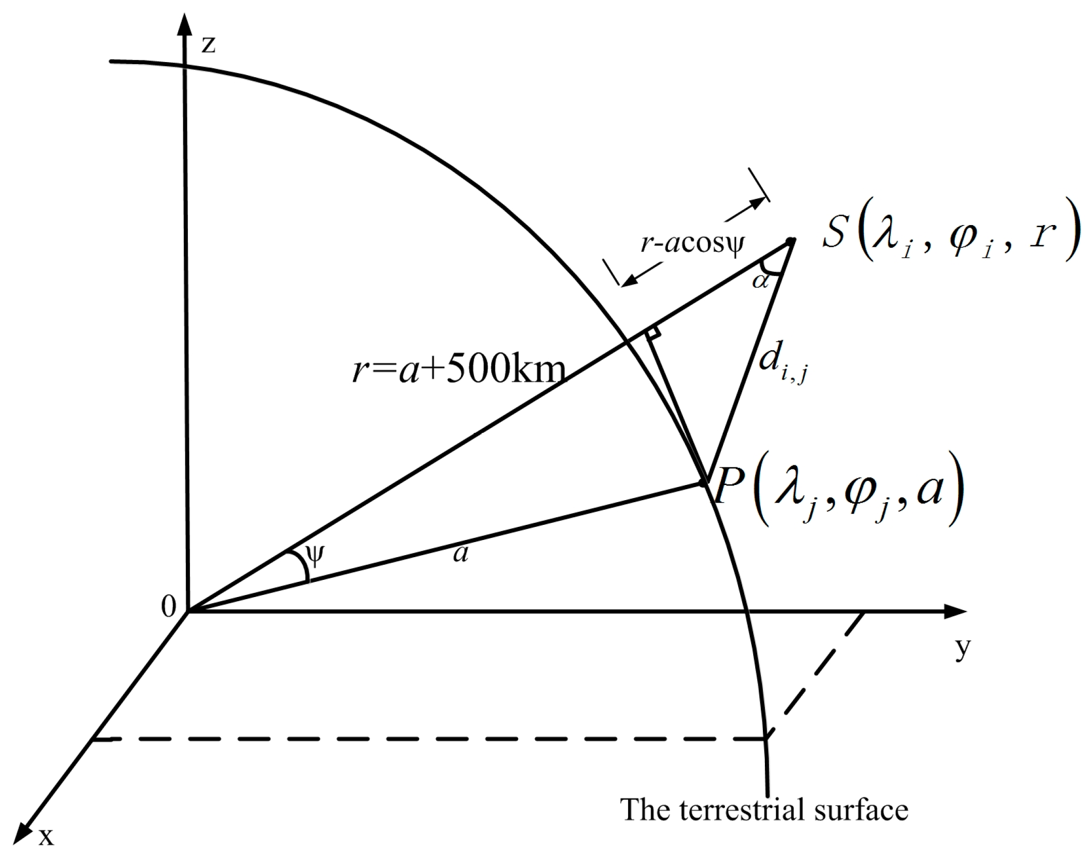
2.3. Mascon Modeling

The mascon model conducted in this research is based on the work of Forsberg and Reeh [14]. The mascon model builds the connection between the mass variations $\delta m_j(j=1,2,\mathrm{...},t)$ on the terrestrial surface of the Earth and the radial gravity disturbance $\delta g_i(i=1,2,\mathrm{...},n)$ at satellite’s attitude.

Figure 2 shows the geometry of the space location $S({\lambda }_i,{\phi }_i,r)$ at the satellite attitude and ground point $P({\lambda }_j,{\phi }_j,a)$, where a point disturbing mass is located; d_i,j is the Euclidean distance between the space location $S({\lambda }_i,{\phi }_i,r)$ and ground location $P({\lambda }_j,{\phi }_j,a)$; ${\psi }_{i,j}$ is the spherical distance between $S({\lambda }_i,{\phi }_i,r)$ and $P({\lambda }_j,{\phi }_j,a)$. According to Newton’s law of gravity, if there are n sampling points at satellite attitude and t mascons in the research area, the total radial gravitational disturbance at each location $S({\lambda }_i,{\phi }_i,r)$ is as follows [15],

$$\delta g_i=G{\displaystyle \sum _{j=1}^t\delta m_j\frac{(r-a\cos {\psi }_{i,j})}{{(a^2+r^2-2ar\cos {\psi }_{i,j})}^{3/2}}},i=1,2,\mathrm{...},n,j=1,2,\mathrm{...},t$$

(4)

where $\delta m_j(j=1,2,\mathrm{...},t)$ is the mascon parameters to be estimated.

Then, we briefly reformulate Equation (4) as the following linear observational equation,

$$y=Ax+e$$

(5)

where y is an n-vector of pseudo observations of radial gravitational disturbance; x is a t-vector of unknown parameters; e denotes the n-vector of random errors with zero mean and variance of unit weight ${\sigma }_0^2$. A is an n × t design matrix, its ith row and jth column element is [15],

$$A\left(i,j\right)=G\frac{(r-a\cos {\psi }_{i,j})}{{(a^2+r^2-2ar\cos {\psi }_{i,j})}^{3/2}},i=1,2,\mathrm{...},n,j=1,2,\mathrm{...},t$$

(6)

Since the pseudo observation vector y is generated from monthly gravity field models using Equation (3), it must be correlated and its covariance matrix D_yy can be derived with the law of error propagation,

$$D_{yy}=B^{T}DB$$

(7)

in which D is the covariance matrix of the Stokes coefficients of monthly model (the variance of C₂₀ is replaced by that from satellite laser ranging data, we use the full covariance matrices of Tongji-GARCE02 monthly solutions, and the diagonal covariance of JPL RL05 and GFZ RL05a monthly solutions as D), B is the coefficient matrix of projecting the Stokes coefficients to the pseudo observation vector, its ith row elements corresponding to Stokes coefficients $\Delta C_{lm}$ and $\Delta S_{lm}$ are written as,

$$\begin{array}{l}B\left(i,j_{\Delta C_{lm}}\right)=-\frac{GM}{r^2}{(\frac{a}{r})}^l\frac{l+1}{1+k_l^{\prime }}{P}_{lm}(\sin {\phi }_i)\cos m{\lambda }_i\\ B\left(i,j_{\Delta S_{lm}}\right)=-\frac{GM}{r^2}{(\frac{a}{r})}^l\frac{l+1}{1+k_l^{\prime }}{P}_{lm}(\sin {\phi }_i)\sin m{\lambda }_i\end{array}$$

(8)

in which, $({\lambda }_i,{\phi }_i,r)$ is the spherical coordinate of ith space location shown in Figure 2, $j_{\Delta C_{lm}}$ and $j_{\Delta S_{lm}}$ are the column numbers corresponding to Stokes coefficients $\Delta C_{lm}$ and $\Delta S_{lm}$, respectively.

2.4. Regularization Solution

Generally, least-squares adjustment is applied to solve the linear equations in order to get best-unbiased estimates. However, the normal matrix N = A^TPA is ill-conditioned (where $P=D_{yy}^{-1}$), which makes the least-squares solution unstable. Therefore, Tikhonov regularization [43,44] is applied to stabilize the solution; its cost function is expressed as:

$$\Phi (x)={(Ax-y)}^{T}P(Ax-y)+\alpha x^{T}Rx=\min$$

(9)

where $\alpha$ indicates the regularization parameter; R is the regularization matrix and here we take R as an identity matrix I. The solution of Equation (5) is,

$$\widehat{x}={(A^{T}PA+\alpha I)}^{-1}{A}^{T}Py$$

(10)

Since the optimal α does not exist theoretically, different methods have been proposed to acquire α, such as the MSE (mean squared error) criterion and the generalized cross-validation method [45]. We apply the MSE criterion that is described in [46,47], because the generalized cross-validation method does not converge in this problem. As for L-curve criterion, Kuche and Klees suggested that it tends to yield over-smooth solutions, especially in the context of satellite-borne gravity field determination [15,48]. We introduce $Q_{\alpha }={(A^{T}PA+\alpha I)}^{-1}$ to simplify the equations, and then the mean squared error matrix can be expressed as follows,

$$MSE(\widehat{x})={\sigma }_0^2{Q}_{\alpha }{A}^{T}PA{Q}_{\alpha }+{\alpha }^2{Q}_{\alpha }\tilde{x}{\tilde{x}}^T{Q}_{\alpha }$$

(11)

which is the combination of the covariance caused by measurement errors and the bias caused by regularization. Since the mean square error of unit weight ${\sigma }_0$ is unknown, we estimate ${\sigma }_0^2$ with the following equation,

$${{\widehat{\sigma }}_0}^2=\frac{{\widehat{e}}^{T}P\widehat{e}-{\alpha }^2{\tilde{x}}^T(Q_{\alpha }-\alpha Q_{\alpha }^2)\tilde{x}}{(n-t)+{\alpha }^{2}tr(Q_{\alpha }^2)}$$

(12)

where $\widehat{e}$ is the estimator of random errors; n and t are the numbers of the measurements and parameters to be estimated, respectively. Since the true value $\tilde{x}$ remains unknown, we replaced them with the estimation $\widehat{x}$. The solution is combined in two steps: (1) a regularized solution $\widehat{x}$ is computed with Equation (10) using a priori regularization parameter α, then applied to Equation (11) as the true value to compute the updated α by minimizing the trace of the mean squared error matrix; and (2) with the updated α, a new regularized solution is produced. The algorithm is terminated while |α_{i + 1} − α_i| < δ, where δ is defined as α/100. The least-squares solutions are treated as the initial values of $\widehat{x}$, since no other reliable estimation is available.

2.5. Leakage Problem

Since signal leakage errors rise proportionally with the strength of signal sources and attenuate rapidly with the increasing distance of signal sources [15], our computed area is about 3 degree larger in all sides than the Tibetan Plateau, which covers a rectangle area of 62°E–108°E, 24°N–48°N. To estimate the leakage errors from outside mass changes of the computed area, we use the additional mascon solutions in surrounding area as the mass change signals, which are computed with the observational Equation (4). The spatial distribution of the trend of leakage errors is presented in Figure 3, in which a positive signal of about 0.2 cm/year occurs in the southern of the Tibetan Plateau, and a negative signal of about −0.6 cm/year occurs in the west of the computed area. Therefore, the leakage errors are corrected in our computation.

3. Mass Flux Solution in Tibetan Plateau

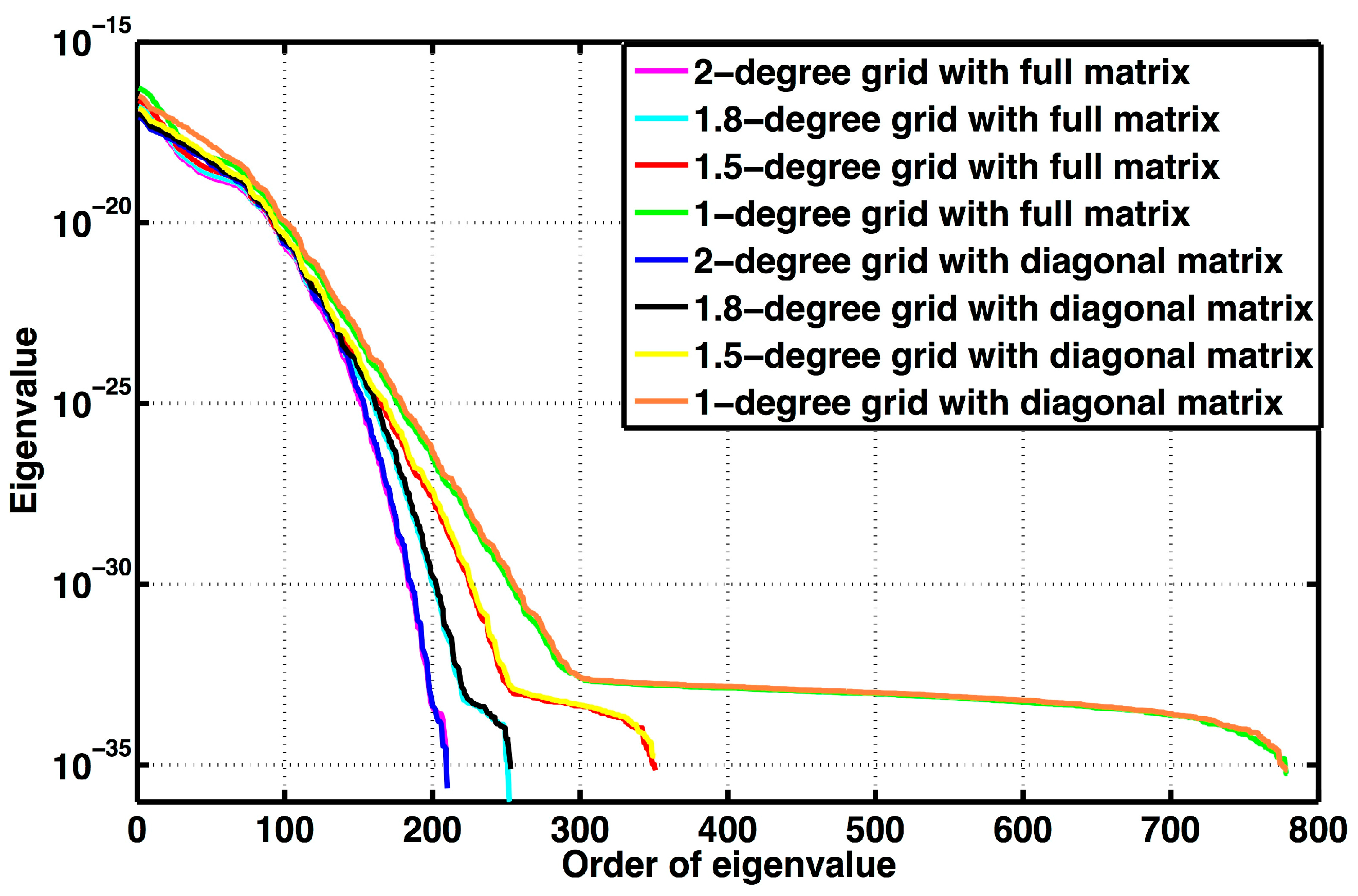
3.1. Spatial Sampling Strategy

The previous works on the mascon models [14,15,49] did not discuss the sampling density of the pseudo observations. The GRACE monthly solutions are truncated to degree/order 60, the correspondent spatial resolution is about 3-degree. A proper sampling density of the pseudo gravitational disturbances at satellite altitude will not only retain observation signals, but also place less computational burden. In order to find proper sampling density of the pseudo gravitational disturbances, their covariance matrices of 2° × 2°, 1.8° × 1.8°, 1.5° × 1.5°, and 1° × 1° grids are investigated, which are computed with Equation (7) using the full covariance matrices of Tongji-GARCE02 monthly solutions D and the diagonal covariance of JPL RL05 and GFZ RL05a monthly solutions published on the ICGEM website (the uncertainties of CSR RL05 is not available). The eigenvalues of the covariance matrices are showed in Figure 4 and Figure 5. Figure 4 presents the eigenvalues computed from both full and diagonal covariance matrices of Tongji-GRACE02 monthly solutions, the results demonstrate that the differences of using full and diagonal covariance matrices are not distinct. However, higher sampling density cannot provide proportional information. In Figure 4, the inflection point of the eigenvalue line of 1° × 1° grid is about 5 × 10⁻³³, more than 400 of the total 779 eigenvalues remain less than this value, which means that most of the pseudo gravitational disturbances cannot provide useful information. For the 1.5° × 1.5° grid, the eigenvalues larger than 5 × 10⁻³³ are much more than those of less than this value, which indicates that its larger eigenvalues are not reduced significantly compared to the total number of eigenvalues. This is the reason we use the 1.5° × 1.5° sampling grid in our computation. The eigenvalues of 1.5° × 1.5° grid from different GRACE monthly solutions (i.e., Tongji-GRACE02, GFZ RL05a, and JPL RL05) in April 2004 are presented in Figure 5, while slight distinctions can be observed among them. The time series of eigenvalues less than 5 × 10⁻³³ from GRACE monthly models for different sampling intervals are presented in Figure 6.

In order to achieve the trend of mass variations in the Tibetan Plateau, we use all available data of CSR RL05, JPL RL05, GFZ RL05a and Tongji-GRACE02 monthly solutions to calculate the pseudo measurements of gravitational disturbance. The Global Land Data Assimilation System (GLDAS) water storage models are converted to Stokes coefficients up to degree and order 60 same as the GRACE monthly solutions and calculated with mascon modeling as well. A total of 312 mascons in the computed area (117 points within the Tibetan Plateau) are recovered by mascon modeling from January 2003 to August 2014. Figure 7 illustrates the location of mascons and mass changes caused by degree-one coefficients. To be noted, for mascons on the boundary of the Tibetan Plateau and only areas within the Tibetan Plateau is calculated in our results. For each month, we establish a set of observation equations in the forms of Equation (5), and no temporal and spatial correlations were introduced. Collecting all the monthly mascon solutions, we constructed the time series of mass flux of terrestrial mascon points and calculated the annual, semi-annual, and 161-day aliasing amplitudes and phases, as well as linear trends based on the least-squares adjustment.

For convenience, the diagonal weight matrices are used for the pseudo observations y of all the GRACE monthly solutions in our mascon modeling in data processing.

3.2. Regularization Parameter

The choice of regularization parameters is the crucial problem to mass flux solution using mascon modeling. Figure 8 presents the trace of mean squared error with respect to regularization parameter ranging from 10⁻²¹ to 10⁻¹⁴, and the regularization parameter for the solution of JPL RL05 in April 2004 is chosen as 2.7 × 10⁻¹⁹ with the minimum trace of mean squared errors. Figure 9 illustrates all regularization parameters for all GRACE solutions, ranging from 10⁻²⁰ to 10⁻¹⁹.

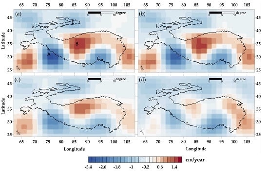
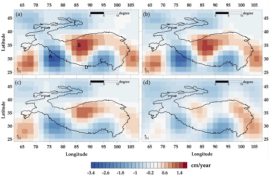
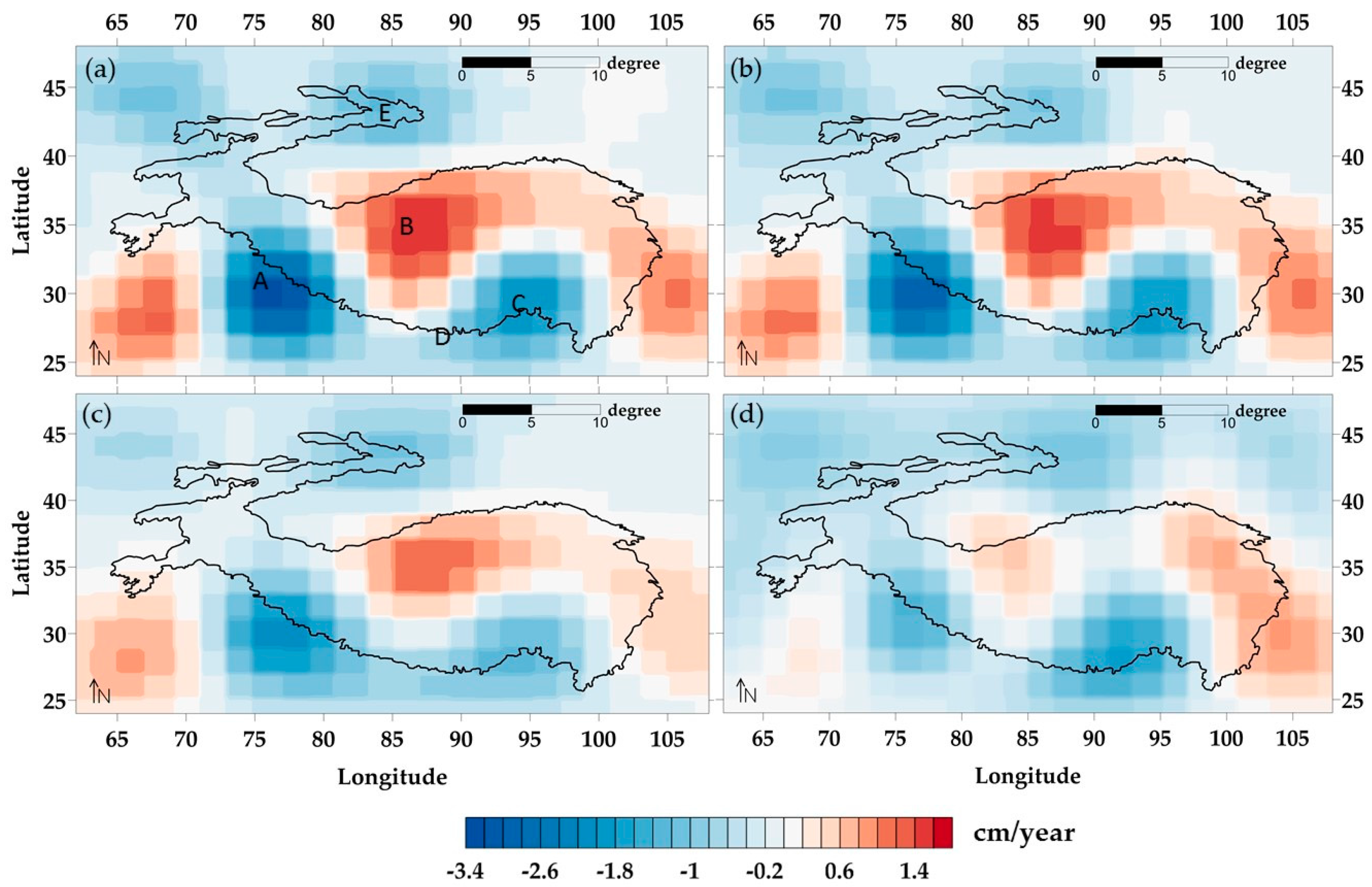
3.3. Spatial Distribution of Tibet

The spatial distributions of mass flux within the rectangular box of Figure 1 with mascon modeling from CSR RL05, JPL RL05, GFZ RL05a and Tongji-GRACE02 monthly solutions are presented in Figure 10. Four strong signals are detected in Figure 10. The strong negative signal centered in 75°E, 30°N (Signal A) is observed, contributed by the North Indian ground water depletion [26,50,51]. CSR RL05 models presented the strongest signal of about −3.4 cm/year in this location, while JPL RL05, GFZ RL05a, and Tongji-GRACE02 produce −2.6 cm/year, −2.2 cm/year and −1.4 cm/year, respectively. In the Inner Tibetan Plateau, a strong positive signal (Signal B) of about 1.4 cm/year is captured, which is believed due to the increasing mass accumulation of numerous high land lakes [25]. However, Tongji-GRACE02 models present only +0.6 cm/year in the same region. Centered in the East Himalayas (95°E, 30°N), another negative signal (Signal C) is detected in all groups’ models. The glacier balance effects contribute the other relatively small signals in the computed area. The results from Tongji-GRACE02 models present a clearer mass loss in the area near 90°E, 27°N (Signal D) and relatively smaller signals over the whole region than those of the other three models. We will discuss this distinction and its causes later in Section 4.3. Signal E stands for the area of Tianshan, in which the decreasing secular trend is found as well.

3.4. Trend of Total Mass Variations

Total mass variations in the Tibetan Plateau resulting from CSR RL05, JPL RL05, GFZ RL05a, Tongji-GRACE02, and GLDAS are drawn in Figure 11, using the time-series of 117 mascons in the Tibetan Plateau. Here we apply the same data processing procedure to the Stokes coefficients expanded from GLDAS and make a comparison, since GRACE and GLDAS contains the same signal source-terrestrial water storage, which is a strong signal in the Tibetan Plateau. GRACE detects all mass change, while GLDAS only contain the top 2–4 m of soil moisture and exclude the anthropology effect [26]. Note that the GLDAS model contains modeling error in the Tibetan Plateau, since it tends to systematically underestimate the surface soil moisture (0–5 cm) while well simulate the soil moisture for 20–40 cm layer [52,53]. Therefore, the amplitude of GLDAS is smaller.

A two-step filtering solution [54] (P₄M₆ decorrelation and 300 km Gaussian filtering) of CSR RL05 is compared with our mascon solution in Figure 12. Clearer annual variations are detected by our mascon solution than the two-step filtering solution.

We establish a fitting function to estimate the bias, linear rate, annual and semi-annual variations, as well as 161-day S₂ alias as follows,

$$EWH(t)=at+b+A_1\cos (\frac{2\pi }{T_1}t-{\theta }_1)+A_2\cos (\frac{2\pi }{T_2}t-{\theta }_2)+A_3\cos (\frac{2\pi }{T_3}t-{\theta }_3),T_1=1,T_2=\frac{1}{2},T_3=\frac{161}{365.25}$$

(13)

where $A_1,A_2,A_3,{\theta }_1,{\theta }_2,{\theta }_3$ stand for the annual, semi-annual and 161-day amplitudes and phases; t is the time tag in years; b is bias parameter. The results of fitting are listed in

Table 2. The annual and semiannual amplitudes, phases of mass flux solution in the Tibetan Plateau.

Models	Annual Amplitude (cm)	Annual Phase (°)	Semiannual Amplitude (cm)	Semiannual Phase (°)
CSR RL05	2.33 ± 0.21	204.83 ± 5.04	0.21 ± 0.17	102.33 ± 49.57
JPL RL05	1.96 ± 0.26	201.74 ± 7.45	0.25 ± 0.10	84.05 ± 74.38
GFZ RL05a	2.19 ± 0.21	208.01 ± 5.16	0.21 ± 0.24	107.30 ± 30.14
Tongji-GRACE02	2.15 ± 0.22	209.93 ± 5.79	0.22 ± 0.28	117.11 ± 31.00
GLDAS	0.56 ± 0.13	167.70 ± 12.83	0.13 ± 0.07	136.84 ± 39.48

and

Table 3. The 161-day amplitudes, phases, and secular trend of mass flux solution in the Tibetan Plateau.

Models	161-Day Amplitude (cm)	161-Day Phase (°)	Trend (Gt/year)
CSR RL05	0.17 ± 0.20	341.00 ± 70.04	−6.41 ± 4.74
JPL RL05	0.10 ± 0.26	277.55 ± 142.72	−5.87 ± 4.88
GFZ RL05a	0.24 ± 0.22	250.04 ± 49.96	−6.08 ± 4.65
Tongji-GRACE02	0.28 ± 0.23	269.42 ± 44.12	−11.50 ± 4.79
GLDAS	0.07 ± 0.13	285.63 ± 249.36	1.90 ± 0.98

. The uncertainties of the fitting are given at 95% confidence level; the secular trend and its uncertainties are corrected by GIA model Pau-5-AUT.

For the GRACE-derived results, the annual amplitudes and phases achieve a fine mutual verification. The annual amplitude of the Tibetan Plateau is around 2 cm and the peak of a year appears at the middle of July, corresponding to the phase of approximately 200°. However, GLDAS produced only 0.56 cm in annual amplitude, while the peak of a year occurs in beginning of June, corresponding to the phase of 167°. The semi-annual amplitudes and phases among different solutions show some difference. The annual amplitude of 161-day S₂ aliasing signal is less than 0.3 cm, which achieves a fine mutual verification with the amplitude computed by CSR RL04 in the same region [55].

The linear rates of 12-year time series show a slight declining trend of the mass flux in the Tibetan Plateau. Tongji-GRACE02 models provide the largest decreasing trend of −11.5 ± 4.79 Gt/year, resulting from the negative signal in Eastern Himalaya and North-Eastern Indian (Signals C and D), and the relatively smaller positive signal in the Inner Tibetan Plateau (Signal B). In particular, the GLDAS solutions provided 1.90 ± 0.98 Gt/year, which might suggest that the terrestrial water storages gain slightly during the time period because of the existence of unknown GLDAS modeling error in this region. Considering the uncertainty of the least squares fitting given at the 95% (2σ) confidence level, and the GIA correction, the terrestrial water storages in the Tibetan Plateau remain stable in the past decade.

We separate the Tibetan Plateau into the mass loss area and mass accumulative area by the values of mass variations and the mass variations are drawn in Figure 13 and Figure 14, respectively. The secular mass accumulative rates are 9.27 ± 2.26 Gt/year for CSR RL05, 8.62 ± 2.29 Gt/year for JPL RL05, 5.17 ± 2.35 Gt/year for GFZ RL05a, and 1.34 ± 2.35 Gt/year for Tongji-GRACE02, respectively. Meanwhile, the secular mass loss rates are −19.09 ± 4.13 Gt/year for CSR RL05, −17.91 ± 4.22 Gt/year for JPL RL05, −14.67 ± 4.10 Gt/year for GFZ RL05a, and −16.26 ± 3.99 Gt/year for Tongji-GRACE02, respectively. If we remove the signal of terrestrial water storage derived from GLDAS (−4.02 ± 0.97 Gt/year) in the mass loss area, the retreating trend of glaciers can be confirmed with the ice-mass change rate of approximately −13.0 ± 2.27 Gt/year.

4. Discussion

4.1. Mass Variations Distribution

As mentioned above, our results show a strong mass loss signal in the northern Indian (−3.4 cm/year as CSR RL05 presented), which was believed to be caused by the India groundwater depletion in the research of Rodell et al. [50]. With the filtering technique, they reported a mean rate of −4.0 ± 1.0 cm/year over the Indian states of Rajasthan, Punjab, and Haryana with GRACE level-2 products from August 2002 to October 2008. Yi and Sun [26] and Jacob et al. [27] found a decreasing rate about 3 cm/year in the identical location as well, which match with our results. Ran et al. produced a linear rate of −2 cm/year in the whole area of North Indian from both Stokes coefficients derived from short-arc approach and dynamic approach and processed a fan filtering [56]; Xing et al. presented a similar distribution using CSR RL04 solutions post-processed by a Gaussian filter [57].

Remote sensing data suggested 68% of observed glaciers in the Himalayas are retreating, while more than 50% observed glaciers in the North-Western Himalaya remains stable or advancing in the early twenty-first century [58,59], which agrees with our results that Signal E remains 0~1 cm/year and there are larger mass losses in the areas of Signals C and D.

The considerable positive signal (1~2 cm/year) in the Inner Tibetan Plateau agrees with the study of Zhang et al. (1~3 cm/year) [60], who suggested that the increasing water masses in lakes in the rate of 4.95 Gt/year caused the gained mass in the Inner Tibetan Plateau with ICESat data. Other GRACE-derived results using filtering method [25,55] and mascon method [27] described in [22] also suggest the mass accumulation in the rate of 1~3 cm/year in the High Mountain Asia region.

On the Tibetan Plateau, the freezing and thawing of permafrost can impact the hydrologic cycle processes by promoting or impeding groundwater and surface water exchange [61], resulting in mass flux detected by GRACE. Permafrost and groundwater dynamics are especially sensitive to climate change. The Inner Tibetan Plateau has been transforming to moist and warm climate patterns, which is revealed by the increasing water levels in the inland lake regions [62]. Our mascon results show the same increasing trend in this region. Meanwhile, the east Himalayas is still controlled by dry and warm climate patterns [62]. The negative signals in the source areas of the Yellow river are related to the diminishing water sources [63], as well as the glacier retreating. Furthermore, since the recharge pathway for the melt water is not known and the local storage capacity of permafrost is limited [27], the difference between our mascon results and sparse mass balance measurements remains to be further discussed. All these interactional factors make the geophysical mechanism in the Tibetan Plateau complicated.

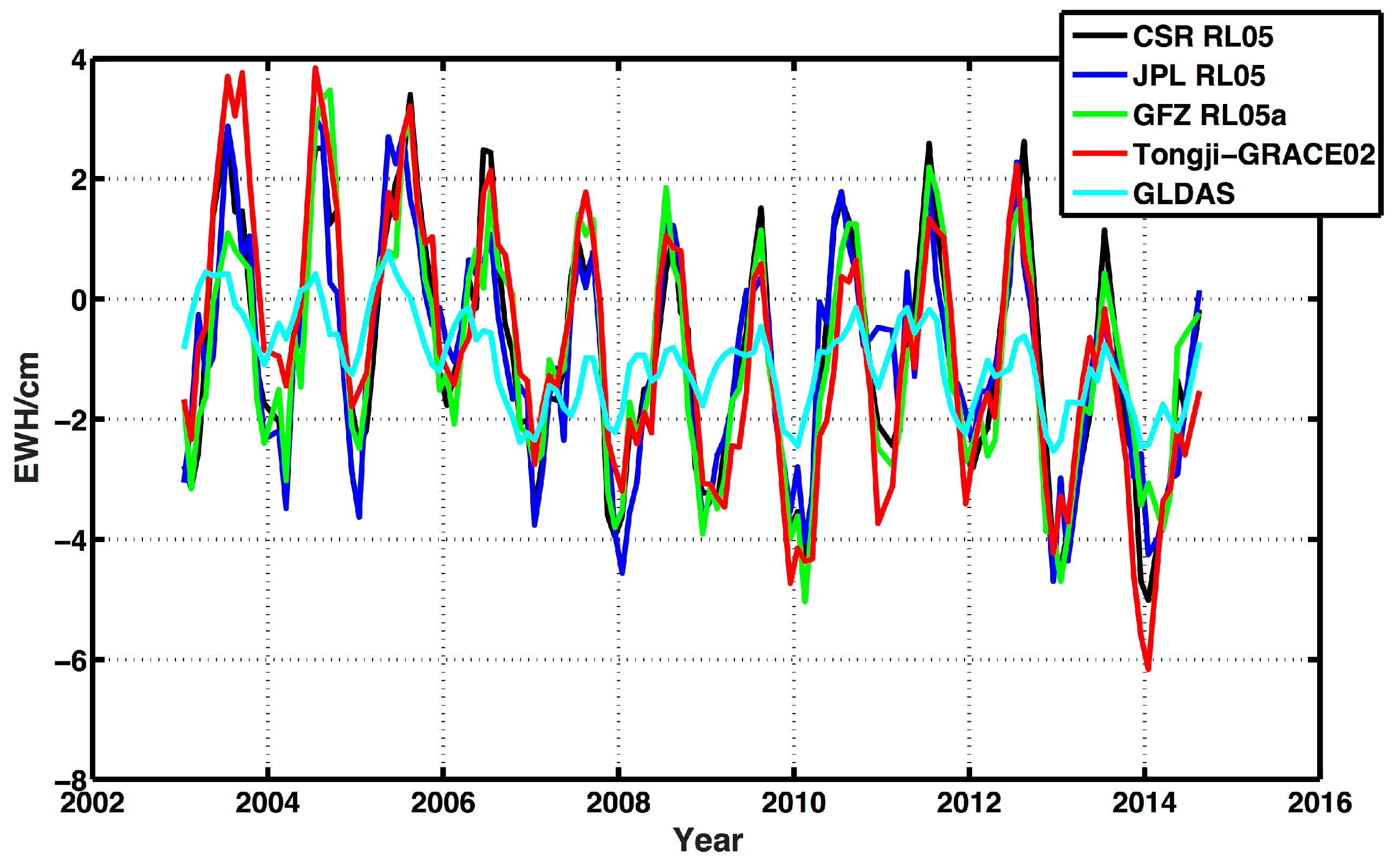
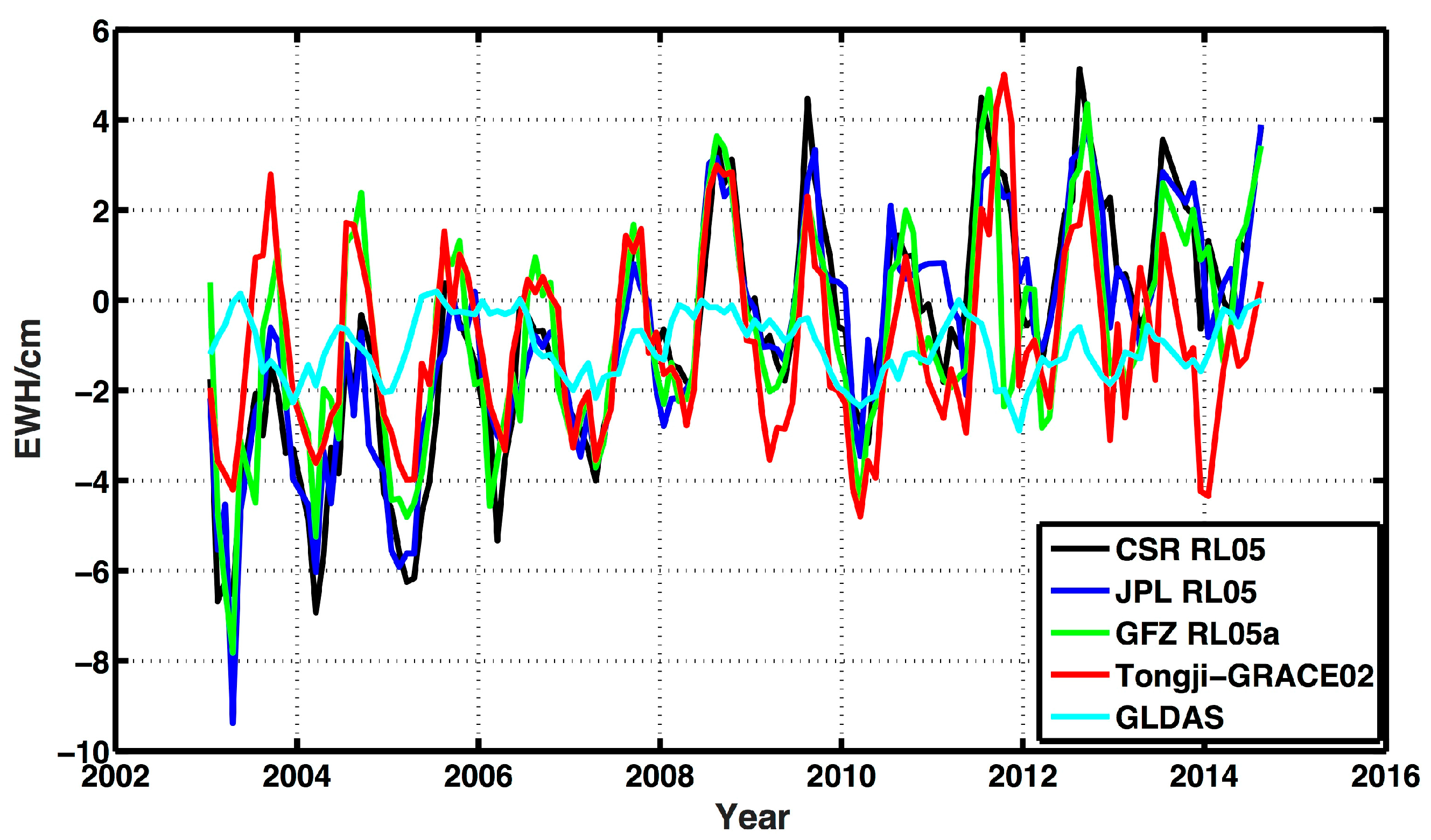
4.2. Total Mass Variation

We have found a downward trend (shown in Table 3) in the Tibetan Plateau. Since other studies concentrate on the ice-mass change rate in the Tibetan Plateau, we remove the hydrology effect estimated by GLDAS from our total mass variation to get the ice-mass change rate, which produces about −7.5 Gt/year. Jacob’s mascon solution produced an ice-mass change rate of −4 Gt/year [27], while Yi and Sun’s spatial filtering solution of −5 Gt/year [26] with the same GIA correction in the same region. Our results are larger than these previous works; the difference may be attributed by the unknown modeling error of GLDAS and the GIA correction.

The linear rate in the Tibetan Plateau of our study is negative, but the long-term mass loss in this area cannot be confirmed, as the decline trend is not significant enough to draw such a conclusion due to the relatively large GIA correction; meanwhile, the uncertainties may be overoptimistic because of the unknown GIA modeling error. Digital elevation models (DEMs) from Shuttle Radar Topography Mission (SRTM) and SPOT 5 stereo imagery were compared in this region, which confirmed slight mass gain or balanced mass budget of glaciers in the central Karakoram, while for the whole Pamir-Karakoram-Himalaya glaciers, a mass balance rate of −0.14 ± 0.08 m/year is reported [56,64].

The GIA correction in this area is about −4 Gt/year with Pau-5-AUT model; however, Yi and Sun suggested that the true value of GIA correction in Tibet might be very small [26]. If we remove the GIA correction from the results of CSR RL05, JPL RL05, GFZ RL05a and GLDAS, the downward trend would not be confirmed based on the uncertainties. Further researches upon the uncertainty of GIA models in this region should be considered.

4.3. Tongji-GRACE02 Monthly Solutions

As Tongji-GRACE02 monthly solutions provide the results with relatively large differences compared to others, the reasons should be well discussed. Tongji-GRACE02 models were developed with modified short-arc approach by modeling the non-conservative acceleration and attitude observation errors [33], while other groups apply a dynamic approach [30,31,32]. Chen et al. suggested that the difference between Tongji-GRACE02 models and others models is contributed by the modeling of the acceleration and attitude data errors, which may absorb parts of signals [65]. The signals of Tongji-GRACE02 model are relatively smaller than other models, especially in the Inner Tibetan Plateau and North India, resulting in the highest secular trend.

The largest negative signal (−1.9 cm/year) of Tongji-GRACE02 is found in 90°E, 25°N (Signal D), which matches with the same signal Dyurgerov predicted (−3.0 cm/year) in the same region with sparse mass balance measurements from 1960 to 2008 [66]. However, there still remains 1.1 cm/year signal or more lost. Jacob et al. [27] attributed the distinction between their results of CSR model and Dyurgerov’s prediction to two geophysical phenomena—the tectonic process and the sinking of the glacier melt water, which seems unlikely. The signal loss is possibly due to the absorption of Signal C, in addition to the accuracy of time-variable gravity field models. Tongji-GRACE02 model may absorb parts of signals because of the modeling method; however, its mass distribution shows its capability of recovering gravitational signals.

5. Conclusions

Mascon modeling is applied in this paper to produce the mass flux solutions in the Tibetan Plateau. For the first time, the covariance of Stokes coefficients is considered to determine the proper sampling density of the pseudo observations. In the Tibetan Plateau, the sampling density of per 1.5° is the most appropriate among all choices.

Mass flux variation distributions in the Tibetan Plateau are presented in this paper. We discovered large mass loss (about −16.9 Gt/year) in Tianshan, North India, and Eastern Himalaya, while a positive signal (about 6.1 Gt/year) in the Inner Tibetan Plateau. The total mass change rate in the Tibetan Plateau from CSR RL05, JPL RL05, GFZ RL05a and Tongji-GRACE02 are −6.41 ± 4.74 Gt/year, −5.87 ± 4.88 Gt/year, −6.08 ± 4.65 Gt/year, and −11.50 ± 4.79 Gt/year, respectively, which indicate mass loss in this area with consideration on the uncertainty of GIA model. Annual amplitude of approximately 2 cm and phases of around 200° are detected in the time series of mass flux in the Tibetan Plateau, which demonstrate that mascon modeling is effective to recovery interannual mass flux. Long-term observations are recommended to recovery the mass flux in the Tibetan Plateau.

References

1. Tapley, B.D.; Bettadpur, S.; Watkins, M.; Reigber, C. The gravity recovery and climate experiment: Mission overview and early results. Geophys. Res. Lett. 2004, 31. [Google Scholar] [CrossRef]
2. Jekeli, C. Alternative Methods to Smooth the Earth’s Gravity Field; Report 327 of Geodetic Science and Surveying; Ohio Ohio State University: Columbus, OH, USA, 1981. [Google Scholar]
3. Wahr, J.; Molenaar, M.; Bryan, F. Time variability of the earth’s gravity field: Hydrological and oceanic effects and their possible detection using GRACE. J. Geophys. Res. 1998, 103, 30205. [Google Scholar] [CrossRef]
4. Zhang, Z.Z.; Chao, B.F.; Lu, Y.; Hsu, H.T. An effective filtering for GRACE time-variable gravity: Fan filter. Geophys. Res. Lett. 2009, 36. [Google Scholar] [CrossRef]
5. Luo, Z.; Li, Q.; Zhang, K.; Wang, H. Trend of mass change in the Antarctic ice sheet recovered from the GRACE temporal gravity field. Sci. China Earth Sci. 2011, 55, 76–82. [Google Scholar] [CrossRef]
6. Sasgen, I.; Martinec, Z.; Fleming, K. Wiener optimal filtering of GRACE data. Stud. Geophys. Geod. 2006, 50, 499–508. [Google Scholar] [CrossRef]
7. Muller, P.M.; Sjogren, W.L. Mascons: Lunar mass concentrations. Science 1968, 161, 680–684. [Google Scholar] [CrossRef] [PubMed]
8. Koch, K.-R.; Morrison, F. A simple layer model of the geopotential from a combination of satellite and gravity data. J. Geophys. Res. 1970, 75, 1483–1492. [Google Scholar] [CrossRef]
9. Koch, K.-R.; Witte, B.U. Earth’s gravity field represented by a simple-layer potential from Doppler tracking of satellites. J. Geophys. Res. 1971, 76, 8471–8479. [Google Scholar] [CrossRef]
10. Koch, K.R. Simple layer model of the geopotential in satellite geodesy. In The Use of Artificial Satellites for Geodesy; Geophysics Monography Series; Henriksen, S.W., Mancini, A., Chovitz, B.H., Eds.; American Geophysical Union: Washington, DC, USA, 1972; Volume 15, pp. 107–109. [Google Scholar]
11. Wong, L.; Buechler, G.; Downs, W.; Sjogren, W.; Muller, P.; Gottlieb, P. A surface-layer representation of the lunar gravitational field. J. Geophys. Res. 1971, 76, 6220–6236. [Google Scholar] [CrossRef]
12. Morrison, F. Algorithms for computing the geopotential using a simple density layer. J. Geophys. Res. 1976, 81, 4933–4936. [Google Scholar] [CrossRef]
13. Russell, R.P.; Arora, N. Global point mascon models for simple, accurate, and parallel geopotential computation. J. Guid. Control Dyn. 2012, 35, 1568–1581. [Google Scholar] [CrossRef]
14. Forsberg, R.; Reeh, N. Mass change of the Greenland ice sheet from GRACE. In Proceedings of the 1st Meeting of the International Gravity Field Service, Istanbul, Turkey, 28 August–1 September 2006.
15. Baur, O.; Sneeuw, N. Assessing Greenland ice mass loss by means of point-mass modeling: A viable methodology. J. Geod. 2011, 85, 607–615. [Google Scholar] [CrossRef]
16. Watkins, M.M.; Wiese, D.N.; Yuan, D.-N.; Boening, C.; Landerer, F.W. Improved methods for observing earth’s time variable mass distribution with GRACE using spherical cap mascons. J. Geophys. Res. Solid Earth 2015, 120, 2648–2671. [Google Scholar] [CrossRef]
17. Luthcke, S.B.; Zwally, H.J.; Abdalati, W.; Rowlands, D.D.; Ray, R.D.; Nerem, R.S.; Lemoine, F.G.; McCarthy, J.J.; Chinn, D.S. Recent Greenland ice mass loss by drainage system from satellite gravity observations. Science 2006, 314, 1286–1289. [Google Scholar] [CrossRef] [PubMed]
18. Luthcke, S.B.; Rowlands, D.D.; Lemoine, F.G.; Klosko, S.M.; Chinn, D.; McCarthy, J.J. Monthly spherical harmonic gravity field solutions determined from GRACE inter-satellite range-rate data alone. Geophys. Res. Lett. 2006, 33. [Google Scholar] [CrossRef]
19. Rowlands, D.D.; Luthcke, S.B.; McCarthy, J.J.; Klosko, S.M.; Chinn, D.S.; Lemoine, F.G.; Boy, J.P.; Sabaka, T.J. Global mass flux solutions from GRACE: A comparison of parameter estimation strategies—Mass concentrations versus Stokes coefficients. J. Geophys. Res. 2010, 115. [Google Scholar] [CrossRef]
20. Sabaka, T.J.; Rowlands, D.D.; Luthcke, S.B.; Boy, J.P. Improving global mass flux solutions from gravity recovery and climate experiment (GRACE) through forward modeling and continuous time correlation. J. Geophys. Res. 2010, 115. [Google Scholar] [CrossRef]
21. Luthcke, S.B.; Sabaka, T.J.; Loomis, B.D.; Arendt, A.A.; McCarthy, J.J.; Camp, J. Antarctica, Greenland and Gulf of Alaska land-ice evolution from an iterated GRACE global mascon solution. J. Glaciol. 2013, 59, 613–631. [Google Scholar] [CrossRef]
22. Rowlands, D.D.; Luthcke, S.B.; Klosko, S.M.; Lemoine, F.G.R.; Chinn, D.S.; McCarthy, J.J.; Cox, C.M.; Anderson, O.B. Resolving mass flux at high spatial and temporal resolution using GRACE intersatellite measurements. Geophys. Res. Lett. 2005, 32. [Google Scholar] [CrossRef]
23. Qiu, J. China: The third pole. Nature 2008, 454, 393–396. [Google Scholar] [CrossRef] [PubMed]
24. Krause, P.; Biskop, S.; Helmschrot, J.; Flügel, W.A.; Kang, S.; Gao, T. Hydrological system analysis and modelling of the Nam Co basin in Tibet. Adv. Geosci. 2010, 27, 29–36. [Google Scholar] [CrossRef]
25. Song, C.; Huang, B.; Ke, L. Modeling and analysis of lake water storage changes on the Tibetan Plateau using multi-mission satellite data. Remote Sens. Environ. 2013, 135, 25–35. [Google Scholar] [CrossRef]
26. Yi, S.; Sun, W. Evaluation of glacier changes in high-mountain Asia based on 10 year GRACE RL05 models. J. Geophys. Res. Solid Earth 2014, 119, 2504–2517. [Google Scholar] [CrossRef]
27. Jacob, T.; Wahr, J.; Pfeffer, W.T.; Swenson, S. Recent contributions of glaciers and ice caps to sea level rise. Nature 2012, 482, 514–518. [Google Scholar] [CrossRef] [PubMed]
28. International Centre for Global Earth Models. Available online: http://icgem.gfz-potsdam.de/ICGEM/ (accessed on 19 May 2016).
29. Bettadpur, S. Gravity Recovery and Climate Experiment UTCSR Level-2 Processing Standards Document for Level-2 Product Release 0005; Center for Space Research, University of Texas at Austin: Austin, TX, USA, 2012. [Google Scholar]
30. Watkins, M.M.; Yuan, D.-N. JPL Level-2 Processing Standards Document for Level-2 Product Release 05; GRACE 327-741, Rev. 4.0; Jet Propulsion Laboratory: Pasadena, CA, USA, 2012. [Google Scholar]
31. Dahle, C.; Flechtner, F.; Gruber, C.; König, D.; König, R.; Michalak, G.; Neumayer, K.-H.; Gfz, D.G. GFZ GRACE Level-2 Processing Standards Document for Level-2 Product Release 0005; Deutsches GeoForschungsZentrum GFZ: Potsdam, Germany, 2013. [Google Scholar]
32. Chen, Q.; Shen, Y.; Zhang, X.; Hsu, H.; Chen, W.; Ju, X.; Lou, L. Monthly gravity field models derived from GRACE level 1b data using a modified short-arc approach. J. Geophys. Res. Solid Earth 2015, 120, 1804–1819. [Google Scholar] [CrossRef]
33. Cheng, M.; Tapley, B.D. Variations in the earth’s oblateness during the past 28 years. J. Geophys. Res. Solid Earth 2004, 109. [Google Scholar] [CrossRef]
34. Hofmann-Wellenhof, B.; Moritz, H. Physical Geodesy, 2nd ed.; Springer-Verlag Wien: New York, NY, USA, 2006. [Google Scholar]
35. Wu, X.; Ray, J.; van Dam, T. Geocenter motion and its geodetic and geophysical implications. J. Geodyn. 2012, 58, 44–61. [Google Scholar] [CrossRef]
36. Swenson, S.; Chambers, D.; Wahr, J. Estimating geocenter variations from a combination of GRACE and ocean model output. J. Geophys. Res. 2008, 113. [Google Scholar] [CrossRef]
37. Cheng, M.K.; Ries, J.C.; Tapley, B.D. Geocenter Variations from Analysis of SLR Data; Springer: Heidelberg, Germany, 2013. [Google Scholar]
38. Peltier, W.R. Ice Age Paleotopography. Science 1994, 265, 195–201. [Google Scholar] [CrossRef] [PubMed]
39. Peltier, W.R. Global glacial isostasy and the surface of the ice-age earth: The ICE-5G (VM2) model and GRACE. Ann. Rev. Earth Planet. Sci. 2004, 32, 111–149. [Google Scholar] [CrossRef]
40. Paulson, A.; Zhong, S.; Wahr, J. Inference of mantle viscosity from GRACE and relative sea level data. Geophys. J. Int. 2007, 171, 497–508. [Google Scholar] [CrossRef]
41. Baur, O.; Kuhn, M.; Featherstone, W.E. GRACE-derived ice-mass variations over Greenland by accounting for leakage effects. J. Geophys. Res. 2009, 114. [Google Scholar] [CrossRef]
42. Wang, H.; Wu, P. Effects of lateral variations in lithospheric thickness and mantle viscosity on glacially induced surface motion on a spherical, self-gravitating Maxwell Earth. Earth Planet. Sci. Lett. 2006, 244, 576–589. [Google Scholar] [CrossRef]
43. Tikhonov, A.N. Solution of incorrectly formulated problems and the regularization method. Sov. Math. Dokl. 1963, 5, 1035–1038. [Google Scholar]
44. Tikhonov, A.N. Regularization of incorrectly posed problems. Sov. Math. Dokl. 1963, 4, 1624–1627. [Google Scholar]
45. Golub, G.H.; Heath, M.; Wahba, G. Generalized cross-validation as a method for choosing a good ridge parameter. Technometrics 1979, 21, 215–223. [Google Scholar] [CrossRef]
46. Xu, P.; Shen, Y.; Fukuda, Y.; Liu, Y. Variance component estimation in linear inverse ill-posed models. J. Geod. 2006, 80, 69–81. [Google Scholar] [CrossRef]
47. Shen, Y.; Xu, P.; Li, B. Bias-corrected regularized solution to inverse ill-posed models. J. Geod. 2012, 86, 597–608. [Google Scholar] [CrossRef]
48. Kusche, J.; Klees, R. Regularization of gravity field estimation from satellite gravity gradients. J. Geod. 2002, 76, 359–368. [Google Scholar] [CrossRef]
49. Ran, J.; Ditmar, P.; Klees, R.; Vizcaino, M. Advanced analysis of mass balance of the Greenland ice sheet from GRACE and surface mass balance modelling. In Proceedings of the 26th IUGG General Assembly, Prague, Czech Republic, 22 June–2 July 2015.
50. Rodell, M.; Velicogna, I.; Famiglietti, J.S. Satellite-based estimates of groundwater depletion in India. Nature 2009, 460, 999–1002. [Google Scholar] [CrossRef] [PubMed]
51. Tiwari, V.M.; Wahr, J.; Swenson, S. Dwindling groundwater resources in northern India, from satellite gravity observations. Geophys. Res. Lett. 2009, 36. [Google Scholar] [CrossRef]
52. Chen, Y.; Yang, K.; Qin, J.; Zhao, L.; Tang, W.; Han, M. Evaluation of AMSR-E retrievals and GLDAS simulations against observations of a soil moisture network on the central Tibetan Plateau. J. Geophys. Res. Atmos. 2013, 118, 4466–4475. [Google Scholar] [CrossRef]
53. Wang, W.; Gao, Y.; Xu, J. Applicability of GLDAS and climate change in the Qinghai-Xizang Plateau and its surrounding arid area. Plateau Meteorol. 2013, 32, 635–645. (In Chinese) [Google Scholar]
54. Chen, J.L.; Wilson, C.R.; Blankenship, D.; Tapley, B.D. Accelerated Antarctic ice loss from satellite gravity measurements. Nat. Geosci. 2009, 2, 859–862. [Google Scholar] [CrossRef]
55. Chen, J.L.; Wilson, C.R.; Seo, K.-W. S2 tide aliasing in GRACE time-variable gravity solutions. J. Geod. 2008, 83, 679–687. [Google Scholar] [CrossRef]
56. Ran, J.; Zhong, M.; Xu, H.Z.; Zhou, Z.; Wan, X. Analysis of the gravity field recovery accuracy from the low-low satellite-to-satellite tracking mission. Chin. J. Geophys. 2015, 58, 3487–3495. [Google Scholar]
57. Lelin, X.; Hui, L.; Songbai, X.; Kaixuan, K.; Xiaoling, L. Long-term gravity changes in Chinese mainland from GRACE and ground-based gravity measurements. Geod. Geodyn. 2011, 2, 61–70. [Google Scholar] [CrossRef]
58. Scherler, D.; Bookhagen, B.; Strecker, M.R. Spatially variable response of Himalayan glaciers to climate change affected by debris cover. Nat. Geosci. 2011, 4, 156–159. [Google Scholar] [CrossRef]
59. Gardelle, J.; Berthier, E.; Arnaud, Y.; Kääb, A. Region-wide glacier mass balances over the Pamir-Karakoram-Himalaya during 1999–2011. Cryosphere 2013, 7, 1263–1286. [Google Scholar] [CrossRef] [Green Version]
60. Zhang, G.; Yao, T.; Xie, H.; Kang, S.; Lei, Y. Increased mass over the Tibetan Plateau: From lakes or glaciers? Geophys. Res. Lett. 2013, 40, 2125–2130. [Google Scholar] [CrossRef]
61. Ge, S.; McKenzie, J.; Voss, C.; Wu, Q. Exchange of groundwater and surface-water mediated by permafrost response to seasonal and long term air temperature variation. Geophys. Res. Lett. 2011, 38. [Google Scholar] [CrossRef]
62. Cheng, G.; Jin, H. Permafrost and groundwater on the Qinghai-Tibet Plateau and in Northeast China. Hydrogeol. J. 2012, 21, 5–23. [Google Scholar] [CrossRef]
63. Jin, H.; He, R.; Cheng, G.; Wu, Q.; Wang, S.; Lü, L.; Chang, X. Changes in frozen ground in the source area of the yellow river on the Qinghai-Tibet Plateau, China, and their eco-environmental impacts. Environ. Res. Lett. 2009, 4. [Google Scholar] [CrossRef]
64. Gardelle, J.; Berthier, E.; Arnaud, Y. Slight mass gain of Karakoram glaciers in the early twenty-first century. Nat. Geosci. 2012, 5, 322–325. [Google Scholar] [CrossRef]
65. Chen, Q.; Shen, Y.; Chen, W.; Zhang, X.; Hsu, H. An improved GRACE monthly gravity field solution by modeling the non-conservative acceleration and attitude observation errors. J. Geod. 2016. [Google Scholar] [CrossRef]
66. Dyurgerov, M.B. Reanalysis of glacier changes: From the IGY to the IPY, 1960–2008. Data Glaciol. Stud. 2010, 108, 1–116. [Google Scholar]
Figure 1. The Tibetan Plateau shown in yellow and the computed area in black rectangular box.
Remotesensing 08 00439 g001
Figure 2. Geometry of mascon modeling.
Remotesensing 08 00439 g002
Figure 3. Trend of the leakage errors estimated with mascons. (a) CSR RL05; (b) JPL RL05; (c) GFZ RL05a; (d) Tongji-GRACE02.
Remotesensing 08 00439 g003
Figure 4. The eigenvalues of the covariance matrices of pseudo observations y in different sampling grid from Tongji-GRACE02 monthly solutions.
Remotesensing 08 00439 g004
Figure 5. Diagonal covariance matrices of Tongji-GRACE 02, GFZ RL05a and JPL RL05 monthly solutions, this figure contains the eigenvalues of the simulated observations’ covariance matrices in the sample density of per 1.5°.
Remotesensing 08 00439 g005
Figure 6. The numbers of eigenvalues less than 5 × 10⁻³³ of monthly solutions with different grid size: (a) JPL RL05; (b) GFZ RL05a; (c) Tongji-GRACE02. (Black: 1° × 1° grid; blue: 1.5° × 1.5° grid; green: 1.8° × 1.8° grid; red: 2° × 2° grid).
Remotesensing 08 00439 g006
Figure 7. Mass changes contributed by degree-1 coefficients (in EWH) and mascons in the computed area. Black dots: mascons outside the Tibetan Plateau; red dots: mascons of the mass accumulative area; green dots: mascons of the mass loss area.
Remotesensing 08 00439 g007
Figure 8. Trace of mean squared errors with respect to regularization parameters.
Remotesensing 08 00439 g008
Figure 9. Regularization parameters of CSR RL05, JPL RL05, GFZ RL05a, Tongji-GRACE02 models.
Remotesensing 08 00439 g009
Figure 10. Spatial distribution of mass flux in Tibetan Plateau: (a) CSR RL05; (b) JPL RL05; (c) GFZ RL05a; (d) Tongji-GRACE02.
Remotesensing 08 00439 g010
Figure 11. Mass variations in Tibetan Plateau after GIA correction.
Remotesensing 08 00439 g011
Figure 12. Mascon solution and two-step filtering solution of CSR RL05 in Tibetan Plateau.
Remotesensing 08 00439 g012
Figure 13. Mass variations in the mass accumulative area after GIA correction.
Remotesensing 08 00439 g013
Figure 14. Mass variations in the mass loss area after GIA correction.
Remotesensing 08 00439 g014