Evaluation of MODIS LAI/FPAR Product Collection 6. Part 2: Validation and Intercomparison

Abstract

The aim of this paper is to assess the latest version of the MODIS LAI/FPAR product (MOD15A2H), namely Collection 6 (C6). We comprehensively evaluate this product through three approaches: validation with field measurements, intercomparison with other LAI/FPAR products and comparison with climate variables. Comparisons between ground measurements and C6, as well as C5 LAI/FPAR indicate: (1) MODIS LAI is closer to true LAI than effective LAI; (2) the C6 product is considerably better than C5 with RMSE decreasing from 0.80 down to 0.66; (3) both C5 and C6 products overestimate FPAR over sparsely-vegetated areas. Intercomparisons with three existing global LAI/FPAR products (GLASS, CYCLOPES and GEOV1) are carried out at site, continental and global scales. MODIS and GLASS (CYCLOPES and GEOV1) agree better with each other. This is expected because the surface reflectances, from which these products were derived, were obtained from the same instrument. Considering all biome types, the RMSE of LAI (FPAR) derived from any two products ranges between 0.36 (0.05) and 0.56 (0.09). Temporal comparisons over seven sites for the 2001–2004 period indicate that all products properly capture the seasonality in different biomes, except evergreen broadleaf forests, where infrequent observations due to cloud contamination induce unrealistic variations. Thirteen years of C6 LAI, temperature and precipitation time series data are used to assess the degree of correspondence between their variations. The statistically-significant associations between C6 LAI and climate variables indicate that C6 LAI has the potential to provide reliable biophysical information about the land surface when diagnosing climate-driven vegetation responses.

1. Introduction

The Leaf Area Index (LAI) and Fraction of Photosynthetically-Active Radiation absorbed by vegetation (FPAR) are two key biophysical variables required by most global models of climate, ecosystem productivity, biogeochemistry, hydrology and ecology [1]. Satellite remote sensing is the most effective way of collecting these variables at a large scale over a long period of time on a regular basis [2]. The MODerate resolution Imaging Spectroradiometer (MODIS) instruments on board NASA’s Terra and Aqua platforms are designed for monitoring the Earth’s atmosphere, ocean and land surface and started operational production and distribution of the LAI/FPAR products from 2000. These datasets are widely used as inputs for land surface models and as training data for neural-network-based LAI/FPAR products, such as GLASS and GEOV1 [3,4]. During the past sixteen years, the MODIS science team aimed to provide users with better products by updating product cohorts, which are called collections. Collection 6 (C6) represents the latest such cohort and contains the entire time series from February 2000 to the present. C6 was released and distributed free of charge to the public from August 2015 and is expected to benefit from improvements of the input data [5].

It is critical to understand the accuracy of the product in order to effectively use LAI/FPAR in land surface models [6,7,8,9,10,11]. There are several schemes to evaluate remote sensing products, including direct validation, intercomparison and other indirect approaches. Many evaluation efforts for previous collections of MODIS LAI/FPAR products can be found in the literature from both the MODIS science team and interested users [9,10,11,12,13]. Special attention has been paid to the accuracy of the estimates, improvements in a new version and consistency with other global products. Collection 5 (C5) products were found to benefit from refinements of algorithm and input data [9]. Intercomparisons with other global products suggested that C5 products are reliable and consistent [8,11]. The main drawbacks of C5 LAI/FPAR were reported to be unrealistically strong temporal variability and systematic overestimation of FPAR over sparsely-vegetated areas [8].

The recently released C6 products have not been validated with ground measurements or compared to existing global products. Thus, it is critical to evaluate the new products, as users are advised to switch to C6. In this context, the primary objectives of this paper are to evaluate the MODIS LAI/FPAR C6 products and to investigate the differences between MODIS products and other global products. This is achieved comprehensively through three approaches: (1) direct validation with ground measurements; (2) intercomparison with GLASS, CYCLOPES and GEOV1 products; and (3) comparison with climate variables.

This paper is organized as follows. Section 2 provides a general description of the datasets used in this study, including global LAI/FPAR products, validation sites and time series of climate variables. Section 3 details three approaches used for validating and intercomparing the LAI/FPAR products. Results and discussion from the various evaluation analyses are documented in Section 4. Concluding remarks are presented in Section 5.

2. Datasets

2.1. Global LAI/FPAR Products

In this section, the main characteristics of the remotely-sensed global LAI/FPAR products under study are described. A brief summary of these characteristics is given in

Table 1. Global LAI/FPAR products investigated in this study. GSD, LUT, RT, GRNN, ANN, tLAI and eLAI stand for “Ground Sampling Distance”, “Look-Up Table”, “Radiative Transfer”, “General Regression Neural Network”, “Artificial Neural Network”, “true LAI” and “effective LAI”, respectively.

Product	GSD	Frequency	Projection	Sensor	Main Algorithm	LAI Type	Ref.
MODIS C5	1 km	8-day	SIN 4	MODIS	LUT based on 3D RT	tLAI	[2,14]
MODIS C6	500 m	8-day	SIN	MODIS	LUT based on 3D RT	tLAI	[5]
GLASS 1 V03	1 km	8-day	SIN	MODIS	GRNN trained with CYC* 5 and MOD 6	tLAI	[3,16]
CYC 2 V3.1	1/112°	10-day	Plate Carrée	VGT	ANN trained with 1D RT	eLAI	[17,18]
GEOV1 3 V1.3	1/112°	10-day	Plate Carrée	VGT	ANN trained with CYC and MOD	Fused with tLAI and eLAI	[4,8]

¹ MODIS period; ² CYCLOPES; ³ VGT period; ⁴ Sinusoidal; ⁵ clumping-corrected CYCLOPES; ⁶ MDOIS.

.

2.1.1. MODIS LAI/FPAR

As described in [2,14], the main algorithm generating the MODIS LAI/FPAR products is based on a three-Dimensional Radiative Transfer (3D RT) model in which atmospherically-corrected reflectances observed by the MODIS instrument and a biome map are used to generate the retrievals. Given daily land surface Bi-directional Reflectance Factors (BRFs) and their uncertainties, the algorithm finds the best LAI and FPAR estimates from biome-specific Look-Up-Tables (LUTs). A back-up empirical method based on the relationships between the Normalized Difference Vegetation Index (NDVI) and LAI/FPAR are utilized to produce estimates with relatively poor quality. LAI and FPAR are produced daily. The LAI value corresponding to the maximum FPAR is selected over the four-day or eight-day compositing period. Vegetation clumping is accounted for at the plant and canopy scales through the model. Therefore, the LAI corresponds to true LAI in all biomes. However, in the case of needle-leaf forest, shoot clumping is not accounted for. The FPAR is defined as the instantaneous black-sky value at the time of the Terra overpass (10:30 a.m.). MODIS products store the corresponding Quality Control (QC) data layers, and the users are advised to consult the quality flags when using these products.

C6 represents the latest version of MODIS LAI/FPAR [5]. The most important change in C6 is that products are being produced at 500-m spatial resolution instead of 1 km, as in C5. A new version of MODIS surface reflectances (MOD09GA C6) is used to replace the previous used 1-km intermediate dataset (MODAGAGG). C6 also replaces the 1-km static land cover input with new multi-year land cover maps at 500-m resolution. From a consistency check of C6 with C5 [5], there are no significant discrepancies between the two collections in terms of global distributions, seasonal variations, interannual LAI anomalies and the spatial coverage of high quality retrievals. A simulation experiment suggested that the differences caused by scale effects are negligible for FPAR and low in the case of LAI [5]. In this study, we only use data from Terra (MOD) instead of Aqua (MYD) or the combined product (MCD) for three reasons: (1) the earlier overpass time of Terra results in more successful retrievals due to low cloud contamination; (2) the GLASS, CYCLOPES and GEOV1 products have a similar acquisition time s Terra; and (3) the GLASS and GEOV1 products have partly been based on MODIS LAI/FPAR from the Terra-MODIS sensor [15].

2.1.2. CYCLOPES LAI/FPAR

The CYCLOPES LAI/FPAR product (http://postel.mediasfrance.org) was produced with data from the SPOT-VGT sensor at 1/112° (about 1 km at the Equator) spatial resolution and a 10-day temporal resolution, in a Plate Carrée projection, for the period 1999–2007 [17,18]. The algorithm used the red, near-infrared and short-wave infrared reflectances, which had been normalized to a standard geometry. LAI and FPAR were estimated using a neural network trained from simulations from a coupled leaf and canopy radiative transfer model (PROSAIL [19]) without using land cover input. Clumping at the plant and canopy scales was not represented in the algorithm, but landscape clumping was represented by considering mixed pixels made of a fraction of pure vegetation and a complement fraction of pure bare soil. Therefore, the LAI corresponds to effective LAI rather than true LAI. The FPAR is defined as the instantaneous black-sky FPAR at 10:00 a.m., referring only to the green elements. The CYCLOPES product was provided with the corresponding error estimate and a quality flag. The early saturation of LAI was reported as the main drawback of the CYCLOPES product [8].

2.1.3. GLASS LAI

The Global Land Surface Satellite (GLASS) LAI dataset was generated and released by Beijing Normal University (http://www.bnu-datacenter.com) [16]. This product has a temporal resolution of eight days and spans from 1982–2012. From 1982–1999, the product was generated from AVHRR reflectances and provided in a geographic projection at the resolution of 0.05°. From 2000–2012, the product was derived from MODIS land surface reflectance (MOD09A1) and provided in a sinusoidal projection at a resolution of 1 km for the globe. In this study, we only focus on the product during the MODIS period. GLASS LAI was derived from reprocessed MODIS reflectance data using General Regression Neural Networks (GRNNs) [3]. GRNNs were trained by a database that was generated from MODIS and clumping-corrected CYCLOPES LAI products over BELMANIP (Benchmark Land Multisite Analysis and Intercomparison of Products) sites during the period from 2001–2003. MODIS LAI and clumping-corrected CYCLOPES LAI were fused in a weighted linear combination in order to obtain the best LAI estimate as follows:

$$LA{I}_{fused}=\omega LA{I}_{mod}+(1-\omega )LA{I}_{cyc}^{*},\text{ with}$$

(1)

$$\omega =f_{mod}/(f_{mod}+f_{cyc})$$

(2)

where, LAI_fused is a combined estimate of LAI, LAI_mod is the smoothed and gap-filled MODIS LAI, LAI*_cyc is the true LAI converted from the CYCLOPES LAI and ω is the normalized weight for the MODIS LAI. Thus, linear regressions were constructed between MODIS and CYCLOPES for each biome type. The weights for each biome were determined by the deviation of MODIS and CYCLOPES (i.e., f_mod and f_cyc) from the ground-measured LAIs. A quality control layer was attached to show the processing status, the quality of inputs and contamination by snow, clouds and shadows.

2.1.4. GEOV1 LAI/FPAR

The GEOV1 LAI/FPAR is the first version of the global biophysical products under the Geoland2 project (http://www.copernicus.eu/projects/geoland2). More than 30 years (1981–present) of the global LAI and FPAR were derived from AVHRR, SPOT-VGT and PROBA-V observations during three temporal periods using neural networks. In this study, we use the product during the VGT-derived period (1998–2014). LAI and FPAR during this period were derived at 1/112° spatial resolution with a 10-day step in a Plate Carrée projection (http://land.copernicus.vgt.vito.be) [4,8]. The MODIS and CYCLOPES products were first fused to obtain the best LAI (same for FPAR) estimate as follows:

$$LA{I}_{fused}=\omega LA{I}_{mod}+(1-\omega )LA{I}_{cyc},\text{ with}$$

(3)

$$\omega =\text{min}(1,\frac{1}{4}LA{I}_{cyc})$$

(4)

where LAI_fused is a combined estimate of LAI, LAI_mod is the MODIS LAI, LAI_cyc is the CYCLOPES LAI and ω is the weight for MODIS LAI. The weight is determined by LAI_cyc and a threshold value (LAI_cyc = 4), which corresponds to the value when CYCLOPES starts to saturate. Neural networks were trained between the fused LAI and the VGT surface directionally-normalized reflectances over BELMANIP sites without biome type specification. Once trained, these networks were run to provide LAI/FPAR every 10 days within the 30-day composite period from the VGT sensor along with quality flags and quantitative uncertainties. The GEOV1 LAI is the combination of true and effective LAI, because MODIS and CYCLOPES LAI correspond to true and effective LAI, respectively. GEOV1 FPAR corresponds to the instantaneous black-sky value around 10:15 a.m. and is calculated by selecting 70% of the cumulative FPAR distribution of daily values within the compositing period instead of the maximum FPAR, as in the case of MODIS [2].

2.2. Validation Sites and BELMANIP Network

The validation dataset is from a collection of sites for which ground measurements have been collected and processed according to the CEOS/WGCV-LPV guidelines [7,20]. An empirical “transfer function” between high spatial resolution radiometric data and the biophysical measurements was used to scale local ground measurements up to the 3 km × 3 km area of the site. There are currently 113 such datasets available, corresponding to sites and various dates of measurements.

The BELMANIP network of sites was designed to represent the global variability of vegetation types and climatological conditions [21]. This network was mainly built using sites from existing experimental networks (FLUXNET, AERONET, VALERI, BigFoot, etc.) and complemented with additionally sites from the GLC2000 land cover map. The site selection was performed for each band of latitude (10° width) by keeping the same proportion of biome types within the selected sites as within the whole latitude band. Attention was paid so that the sites were homogeneous over a 10 × 10 km² area, almost flat and with a minimum proportion of urban area and permanent water bodies. Note that there are no ground measurements for most of these sites, and therefore, this network is always used for intercomparison, rather than direct validation. Representing the latest version, the BELMANIP2.1 currently contains 445 sites and is used in this study.

2.3. Time Series of Climate Variables

This study uses the Time Series (TS) datasets of global surface temperature and precipitation that were produced by the Climatic Research Unit (CRU) at the University of East Anglia [22]. Climate variables were calculated for each 0.5° × 0.5° latitude/longitude grid, monthly, by employing a triangulated linear interpolation method. Through the auspices of the World Meteorological Organization (WMO) in collaboration with the U.S. National Oceanographic and Atmospheric Administration (NOAA), archives provided by more than 4000 meteorological stations were used to cover the world’s land areas. At present, the latest time series data (TS 3.23) were generated by the CRU for the period 1901–2014 and publicly available from http://www.cru.uea.ac.uk.

3. Methodology

3.1. Direct Validation with Ground Measurements

3.1.1. Selection of Reliable Ground Measurements

We use the spatially-averaged values over a 3 km × 3 km reference map as the “ground truth” at each validation site, as in previous studies [7,8]. However, several sources of uncertainties reduce the reliability of these measurements. First, optical instruments (e.g., LAI2000) that are generally used for point-scale measurements only provide effective LAI (eLAI), which may result in an underestimation of true LAI (tLAI) [23] up to 70% in coniferous forests [24]. Second, the scale effect in indirect ground measurement can result in obvious uncertainties when the sampling length is not properly selected and this has often been ignored [25]. Third, the up-scaling scheme using an empirical ‘‘transfer function’’ between high spatial resolution reflectances and point-scale biophysical measurements requires a relatively large homogenous area, which may not be satisfied at some sites. Last but not least, uncertainties can arise due to the effects of the point spread function and geo-location errors of the satellite pixel. The overall uncertainty at each site differs with vegetation type, surface homogeneity, equipment used, sampling strategy, etc. [26]. However, absolute uncertainties of LAI reference maps corrected for clumping and non-green elements are expected to be smaller than 1 LAI unit in most sites [27]. The uncertainty is expected to be around 0.1 for FPAR [8].

Figure 1 shows the biome type distribution within each 3 km × 3 km validation site based on the MODIS land cover product (500-m resolution, C5). The upper part of the plot denotes the information entropy of the biome type for each site. This serves as an indicator of surface homogeneity. The information entropy is calculated using the proportion of each biome type within a specific site as follows:

$$H=-{\displaystyle \sum }_{\mathrm{i}=1}^{11}({\mathrm{P}}_{\mathrm{i}}*{\text{log}}_2{\mathrm{P}}_{\mathrm{i}})$$

(5)

where H is information entropy and ${\mathrm{P}}_{\mathrm{i}}$ represents the proportion of the area covered by the i-th biome type. The value 11 corresponds to the total number of MODIS land cover types. We screened out some of the 113 sites to improve the overall accuracy of these measurements. This screening was based on four criteria: (1) Presence of 500 m × 500 m pixels labeled as “water” with the 3 km × 3 km site; (2) the information entropy of biome type was greater than 1; (3) the proportion of invalid MODIS pixels (based on QC in

Table 2. Quality control for the four products under study.

Product	Quality Flag	Snow	Cloud	Shadow	Aerosol	Cirrus	Suspect	Overall
MODIS	FparLaiQC	Clear	Clear	-	No	No	-	-
	FparExtraQC	-	Clear	Clear	-	-	-	Good
GLASS	QC	Clear	Clear	Clear	-	-	-	Good
CYCLOPES	SM	Clear	-	-	Pure	-	No	Good
GEOV1	QFLAG	Clear	-	-	Pure	-	No	Good

) was larger than 40%; and (4) suspicious LAI/FPAR values (e.g., LAI < 2 for dense forests, Site #42) based on field experience and literature reports [8].

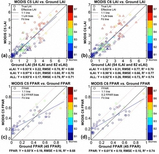
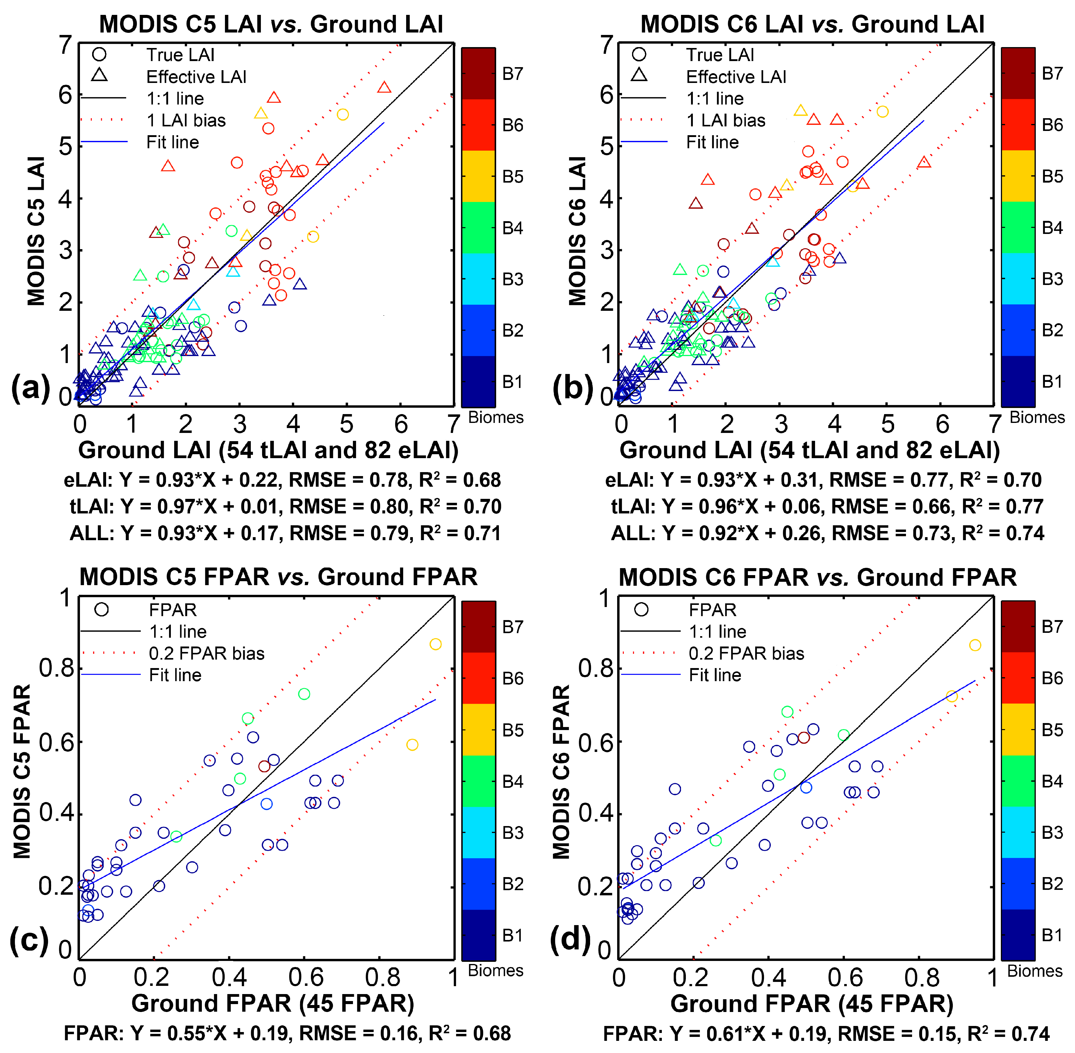
3.1.2. Validation of MODIS LAI/FPAR Product

We compared both MODIS C5 and C6 products with ground measurements. The spatial and temporal mismatch between the remote sensing product and ground truth is the main issue related to such a comparison [4,18]. A 3 × 3 array of surrounding pixels has been recommended for calculating the mean value to reduce geolocation uncertainties [8]. Considering that reference maps cover a 3 km × 3 km area, which contains about 36 (6 × 6) MODIS C6 pixels and 9 (3 × 3) C5 pixels, we averaged all of the valid pixels within the reference map. The corresponding 8-day composite, which includes the date of ground measurements was extracted. Thus, the maximum temporal mismatch is about 7 days, which should have minimal impact in most cases. Compared to the overall uncertainties of the LAI reference maps, uncertainties caused by spatial and temporal mismatch may be thus ignored. As suggested by the MODIS product user guide, the QC layers were consulted to exclude retrievals with poor quality caused by snow, clouds or high aerosol content (details in Section 3.2.1). Only retrievals from the main algorithm were used for the validation analyses reported here.

3.2. Intercomparison with Existing Global Products

3.2.1. Quality Control for Products

All of the four products under study provide QC layers, and users are advised to consult the quality flags when using them. Therefore, we performed quality control for each product using the criteria listed in Table 2. In agreement with other studies [6,7,8,10,18], land pixels contaminated by clouds or marked as “snow”, “aerosol”, ”cirrus” or “suspected” according to the QC information were marked as invalid data. Note that quality control for different products was not identical because of different QC layers. For instance, MODIS and GLASS were masked by cloud, while CYCLOPES and GEOV1 were not. The MODIS biome map was used to exclude bare areas from this analysis. This study used retrievals from both the main and back-up algorithms in order to show the performance of the products instead of algorithms.

3.2.2. Comparison of Spatial Distribution

This study evaluated the four global LAI/FPAR products at the continental and global scale to characterize their performances. These products must be resampled to an identical projection and period to enable pixel-by-pixel comparisons. The four products were first quality controlled as described in Section 3.2.1 and then resampled to the Plate Carrée projection with a quarter degree spatial resolution. The LAI/FPAR values for each 0.25° × 0.25° pixel were computed as the average of all valid native pixels falling within the coarser grid. A no-data value was assigned if more than 30 percent of the native pixels were composed of invalid data (based on QC in Table 2). The datasets with different temporal compositing periods were averaged into a monthly time step. The pixel was assigned with a no-data value if there were no valid data within the whole month.

Pixel-by-pixel absolute differences (MODIS minus other products) between MODIS and the other three LAI products and other two FPAR products were calculated and mapped at the global scale for visual comparison. Histograms of global LAI and FPAR from each product were computed and compared. Two particular months—January and July in 2001—were selected to represent the boreal winter and summer, respectively. In addition, the spatial consistency of LAI over the African continent was investigated. As in [7], we extracted and compared latitudinal LAIs from the four products along the longitudes between 20° E and 25° E.

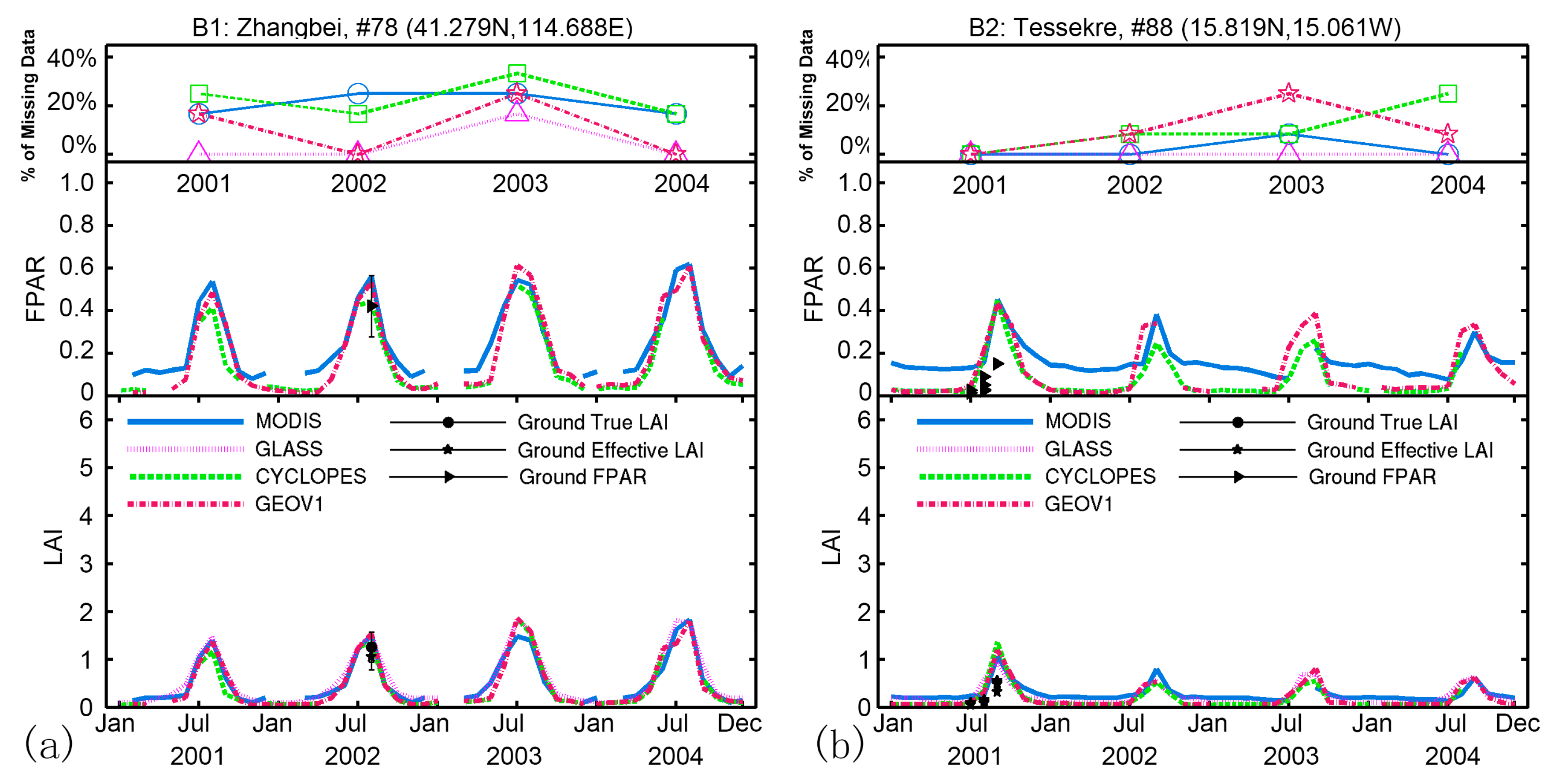
3.2.3. Comparison at the Site Scale

We compared four LAI products and three FPAR products over 445 BELMANIP2.1 sites. Products were masked by QC flags and aggregated into a monthly time step. LAI and FPAR values from the 60 months of the 2001–2005 period were used to assess the discrepancies between different products through scatterplots. In this exercise, the original projections of the products were kept, and a 1-km (for MODIS and GLASS) or 1/112° (for CYCLOPES and GEOV1) spatial resolution was adapted. This is because of two reasons: (1) the high homogeneity of these sites reduces the geolocation uncertainties due to different projection systems, target shift and different point spread functions [21]; and (2) any additional processing including reprojection and resampling would introduce more uncertainties [6].

The MODIS land cover map was used to divide the 445 sites into three broad vegetation classes in terms of canopy structure and leaf shape. The three classes are non-forest (Biomes 1–4), broadleaf forests (Biomes 5 and 6) and needleleaf forests (Biomes 7 and 8). Regression equations for any two products, as well as the corresponding coefficient of determination (R²) and root-mean-squared error (RMSE) were computed to assess the consistency.

3.2.4. Temporal Comparison

We evaluated temporal LAI/FPAR profiles of the four products extracted over seven validation sites where some ground measurements were available during the period from 2001–2004. Each site represented one vegetation type in the MODIS classification scheme. There was no validation site that could be used for DNF. Monthly LAI/FPAR estimates were first calculated using the same approach described in Section 3.2.3. Then, the seasonal variations of the four products were compared for both LAI and FPAR with R² and RMSE denoting the consistency.

3.3. Comparison with Climate Variables

Using independent geographic variables to explain the interannual variations of LAI/FPAR is a novel approach of indirectly evaluating these products. Due to a lack of long-term data, this evaluation method has not been used for MODIS LAI/FPAR previously. In this study, we applied this approach using thirteen years (2002–2014) of MODIS C6 LAI data. 2000 and 2001 were not included because of the missing data in these two years. The C5 and C6 LAI products were firstly resampled to the Plate Carrée projection and aggregated to a half degree spatial resolution and a monthly time step. QC information was taken into account to exclude retrievals with poor quality. In this manner, the LAI dataset matched the datasets of climate variables both spatially and temporally. Further averaging over some specific regions and over the whole year or some specific months was done to obtain the time series for statistical analyses. An area-weighted approach was used to eliminate geometrical effects. Anomalies of LAI, temperature and precipitation were computed by subtracting the thirteen-year mean from data of specific years. We calculated standardized anomalies (anomalies normalized by their standard deviations) of LAI and surface temperature during the beginning of the growing season (April and May) for four temperature-limited regions within 60°N–90°N. We also calculated standardized anomalies of annual averages of LAI and precipitation for two water-limited regions. In addition, the correlation between annual averaged LAI and annual total precipitation in the tropical latitudes (23° S–23° N) was investigated.

4. Results and Discussion

4.1. Direct Validation

4.1.1. Characteristics of Measurements

As mentioned above, the validation data used in this paper is from a collection of sites all over the world. Therefore, the method of ground measurement (e.g., destructive sampling, LAI-2000, digital hemispherical photos, TRAC, AccuPAR and allometry) may vary from site to site and from date to date. Details of these sites can be found on http://calvalportal.ceos.org/web/olive. Note that effective LAI measured by optical instruments may differ significantly from true LAI, particularly in forests [24]. These indirect measurements that have been corrected for clumping effect are also considered as true LAI in this study. Measurements without clumping correction were discarded in some studies [7,8], but were investigated separately in this study. We also compared the MODIS FPAR with ground measurements, which was seldom done in previous studies. Measurements at the same site, but different dates were considered independently.

Table 3. Biome-specific information of ground measurements after pre-selection. The numbers of ground measurements of tLAI, eLAI and FPAR for each biome are listed. The mean values and standard deviations of both ground measurements and retrievals from the C5 and C6 products are also provided (mean value ± standard deviation).

Biome Type	# of tLAI	Ground tLAI	MODIS C5 LAI	MODIS C6 LAI	# of eLAI	Ground eLAI	MODIS C5 LAI	MODIS C6 LAI	# of FPAR	Ground FPAR	MODIS C5 FPAR	MODIS C6 FPAR
B1 1	12	1.37 ± 1.01	1.20 ± 0.80	1.32 ± 0.85	49	0.93 ± 0.94	0.83 ± 0.50	0.94 ± 0.62	36	0.26 ± 0.24	0.32 ± 0.14	0.33 ± 0.16
B2 2	2	0.18 ± 0.19	0.21 ± 0.01	0.21 ± 0.01	1	0.03 ± 0.00	0.20 ± 0.00	0.20 ± 0.00	2	0.26 ± 0.34	0.28 ± 0.21	0.31 ± 0.24
B3 3	0	N/A	N/A	N/A	3	2.14 ± 0.75	2.09 ± 0.43	2.14 ± 0.55	0	N/A	N/A	N/A
B4 4	15	1.61 ± 0.55	1.43 ± 0.69	1.46 ± 0.47	15	1.26 ± 0.36	1.43 ± 0.69	1.46 ± 0.47	4	0.44 ± 0.14	0.56 ± 0.18	0.53 ± 0.15
B5 5	2	4.65 ± 0.39	4.44 ± 1.66	4.65 ± 0.39	2	3.27 ± 0.18	4.44 ± 1.66	4.95 ± 1.02	2	0.92 ± 0.04	0.73 ± 0.20	0.79 ± 0.10
B6 6	14	3.58 ± 0.40	3.77 ± 0.99	3.79 ± 0.82	7	3.78 ± 1.26	4.74 ± 1.10	4.67 ± 0.59	0	N/A	N/A	N/A
B7 7	9	2.69 ± 0.76	2.58 ± 1.08	2.42 ± 0.73	5	1.72 ± 0.48	2.31 ± 0.80	2.60 ± 0.97	1	0.49 ± 0.00	0.53 ± 0.00	0.61 ± 0.00
B8 8	0	N/A	N/A	N/A	0	N/N	N/A	N/A	0	N/A	N/A	N/A
Overall	54	2.31 ± 1.26	2.25 ± 1.46	2.28 ± 1.38	82	1.37 ± 1.21	1.49 ± 1.36	1.59 ± 1.35	45	0.31 ± 0.27	0.36 ± 0.18	0.38 ± 0.19

¹ Grasses/cereal crops; ² shrubs; ³ broadleaf crops; ⁴ savanna; ⁵ EBF; ⁶ DBF; ⁷ ENF; ⁸ DNF.

shows biome-specific information of ground measurements after pre-selection, as described in Section 3.1.1. The mean values and standard deviations of both ground measurements and retrievals from C5 and C6 products are provided. After pre-selection, there are 54 true LAI, 82 effective LAI and 45 FPAR measurements left for further analyses. Note that there are no valid true LAI and FPAR measurements for broadleaf crops, and there are no FPAR measurements for DBF. We also lack LAI and FPAR measurements for DNF. The absence of a valid ground truth suggests that more field measurements are needed in the future to further refine this assessment. Ground measurements and MODIS estimates indicate the same vegetation density sequence: broadleaf forests > needleleaf forests > savannas > grasses/cereal crops > shrubs. LAI/FPAR values extracted from the C5 and C6 products show good agreement in all vegetation types. The slight overestimation in C6 relative to C5 is due to scale effects and refinements to surface reflectances [5]. C5 shows the most obvious underestimation in savanna, which is in agreement with [28]. This issue has been mitigated by C6 to some extent. We note that MODIS LAI overestimates the ground measurements in DBF, which was also reported by [8]. As expected, effective LAIs are lower than true LAIs for all biomes due to the lack of correction for clumping. MODIS LAI estimates are found to be closer to true LAI rather than effective LAI. The largest difference between measured LAI and C5 is achieved in EBF. However, this difference is corrected in C6. Considering all biomes, measured LAI (2.31) agrees with C6 (2.28) better than with C5 (2.25). Broadleaf forests show large differences between measured effective LAI and MODIS estimates, which is due to the unneglectable clumping effects. MODIS FPAR shows overestimation in all biomes, except for EBF, where radiative signals may saturate.

4.1.2. Comparison with Ground Measurements

Figure 2a,b compares measured LAI with MODIS C5 and C6 LAI, respectively. As expected, MODIS shows better agreement with true LAI than with effective LAI. MODIS retrievals are found to systematically overestimate effective LAI measurements, especially in forests, which agrees with Stenberg et al. [29], who suggested that an effective LAI can produce errors of 30%–70%. In comparison with true LAI measurements, C6 performs better than C5 with the RMSE decreasing from 0.8 down to 0.66 and R² increasing from 0.70–0.77. Large uncertainties are found in high LAI values, which can be explained by relatively lower algorithm accuracy due to signal saturation. Overall, most of the data are within ±1 LAI bias, indicating that the total uncertainty of this validation work is less than 1 LAI unit. Note that this uncertainty comes from both MODIS products and other sources, including the uncertainties of reference maps and mismatch in spatial and temporal domains. We also note that the distribution of the measurements is problematic with an over-representation of low values. This is expected to be solved by adding more ground measurements, especially for broadleaf crops and forests, according to the CEOS/WGCV-LPV guidelines.

In comparisons to ground measurements, MODIS FPAR performs relatively poorly compared to LAI (Figure 2c,d). The RMSE of C5 and C6 are 0.16 and 0.15, respectively. The R² increases from 0.68–0.74 from C5 to C6. We notice a significant overestimation of MODIS retrievals in both C5 and C6 at low FPAR values. This systematic overestimation of FPAR over sparsely-vegetated areas was reported as a main drawback of the MODIS FPAR product [8]. However, the disagreement in this study may also be due to the fact that understories are usually not taken into account in ground measurements, which will underestimate the true FPAR [15]. Overall, most data are within ±0.2 bias with all uncertainties included.

4.2. Intercomparison

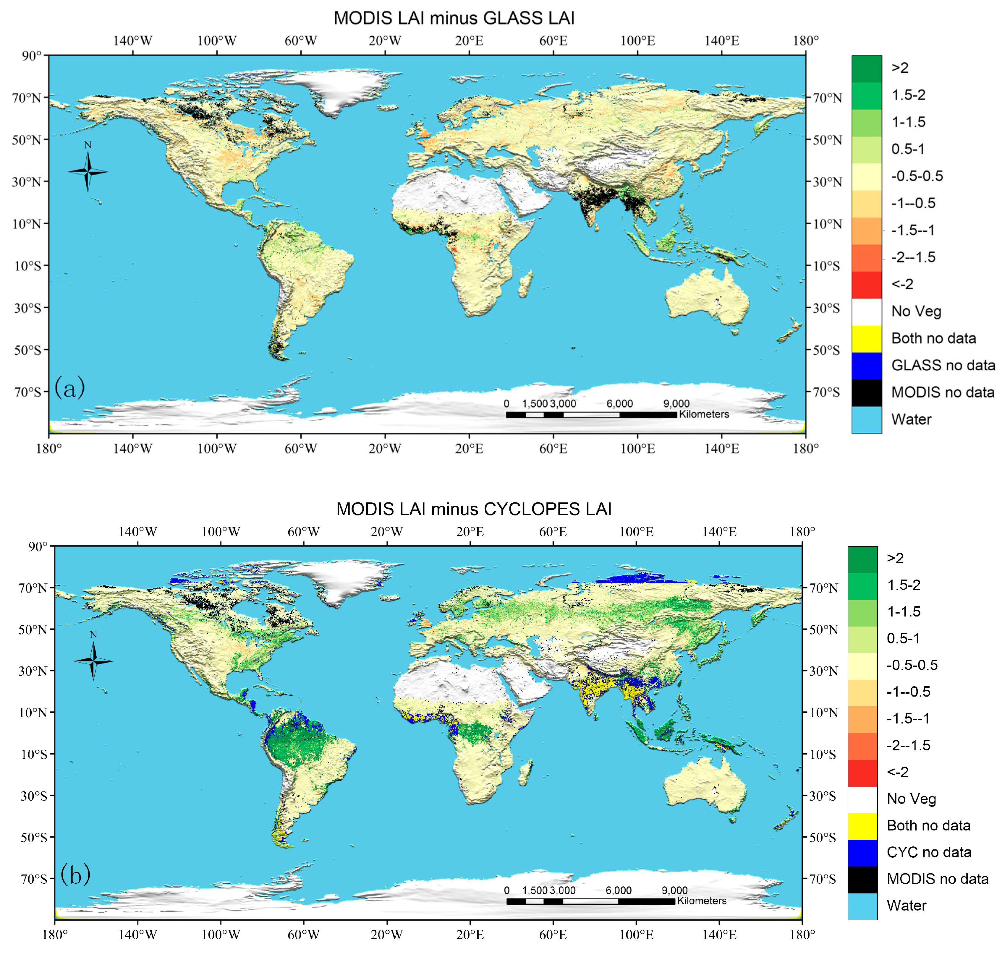
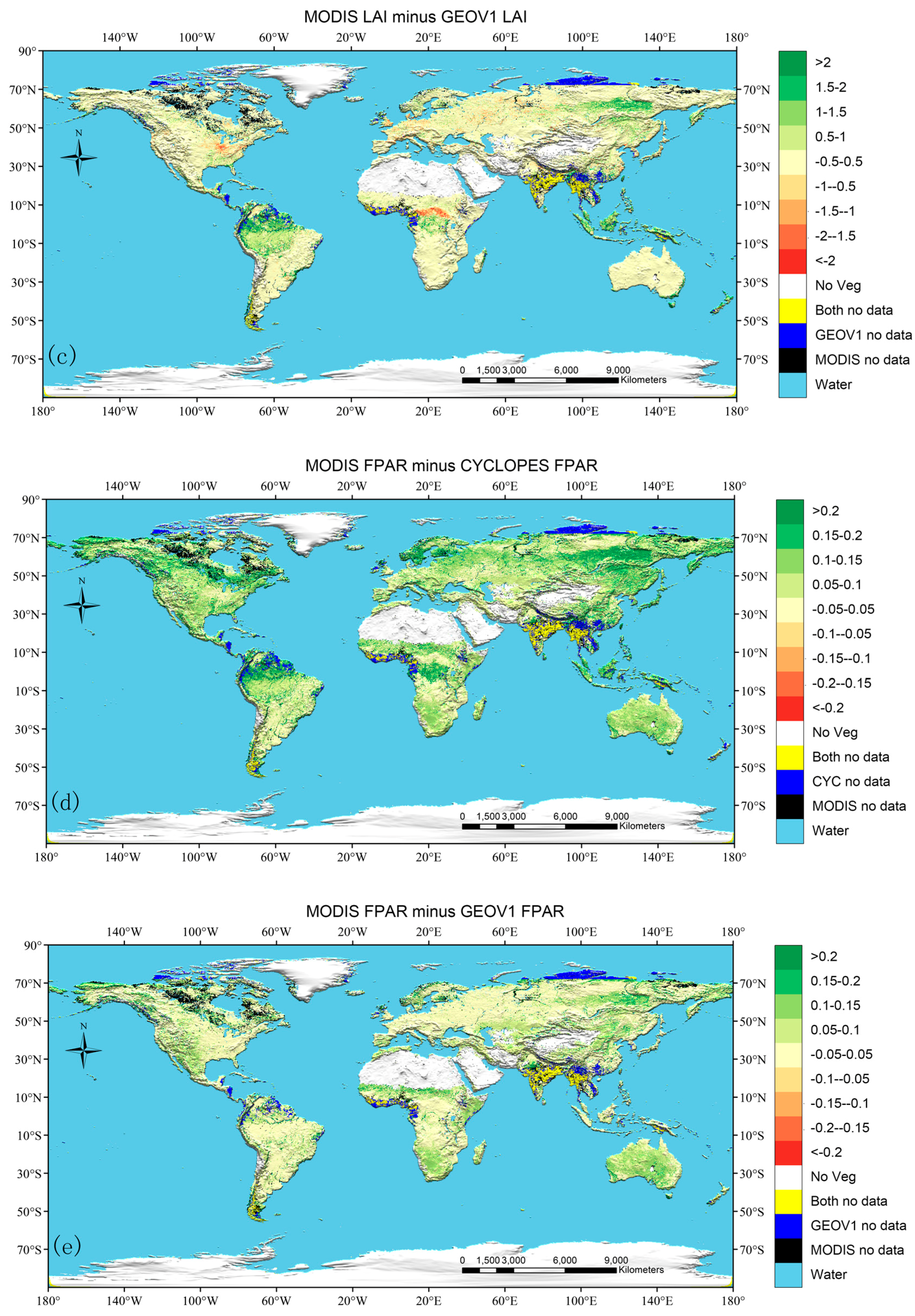
4.2.1. Global LAI/FPAR Distribution

Figure 3a–c displays the global distribution of absolute LAI differences between MODIS and three other products in July 2001. Figure 3d,e shows the corresponding FPAR. As expected, the four products generally show a continuous LAI/FPAR distribution at the global scale. We notice that CYCLOPES and GEOV1 do not provide LAI or FPAR estimates at high latitudes (>74°) due to the absence of SPOT-VGT observations in these regions. South Asia and Southeast Asia are the largest regions with missing data for MODIS, CYCLOPES and GEOV1. This is caused by the frequent cloudy weather related to the southwest monsoon in these regions [30]. The reason why the GLASS product has valid data is due to gap-filling. MODIS also has missing data over the high latitudes of North America due to cloud contamination or poor atmospheric conditions.

MODIS is found to agree best with GLASS, as expected, with absolute differences within ±0.5 LAI units for most of the land surface (Figure 3a). The reasons are two-fold: (1) the surface reflectance data input to the two algorithms are from the same MODIS instrument; (2) MODIS LAI products are used as one part of the ANN training data for GLASS. Compared to GLASS, most overestimation of MODIS LAI is seen in tropical densely-vegetated regions. From Figure 3b,d, we notice significant underestimation from CYCLOPES, especially in densely-vegetated regions. These discrepancies between MODIS and CYCLOPES can reach to two for LAI and 0.2 for FPAR. This result agrees with previous studies and was found related to premature saturation in the CYCLPOES algorithm [7,8]. This issue was reportedly solved in GEOV1 by using the MODIS product as the training data when LAI is larger than four [4]. Indeed, we find that MODIS agrees better with GEOV1 than CYCLOPES. However, GEOV1 still shows underestimation in some regions, e.g., forests in the Amazon and South Asia. Note that the distributions of discrepancies between MODIS and GEOV1 are not consistent for LAI and FPAR.

In Figure 4a,b, the four products show smooth and consistent LAI distributions at the global scale for both January and July. Differences between global distributions are smaller in January than in July, indicating that most inconsistency occurs during the growing season of northern latitudes. The global mean LAIs calculated from MODIS, GLASS, CYCLOPES and GEOV1 are 1.42, 1.43, 1.02 and 1.15 in January and increase to 2.02, 2.09, 1.53 and 1.81 in July, respectively. Note that the number of valid overlapping pixels also increases from 96,346 in January to 180,603 in July. This increase is caused by better atmospheric conditions and less cloud or snow contamination in the boreal summer season. Unlike other products, CYCLOPES shows a peak at around LAI = 2.5 and drops rapidly to zero after LAI = 4 in July, which confirms the early saturation issue reported previously. Compared to LAI, FPAR discrepancies are found to be relatively larger (Figure 4c,d). The global mean FPARs calculated from MODIS, CYCLOPES and GEOV1 are 0.4, 0.31 and 0.35 in January and increase to 0.54, 0.43 and 0.5 in July, respectively. The frequency of low LAI and FPAR values is considerably smaller for MODIS than for other products, which is due to the overestimation of the MODIS product in sparsely-vegetated regions [7].

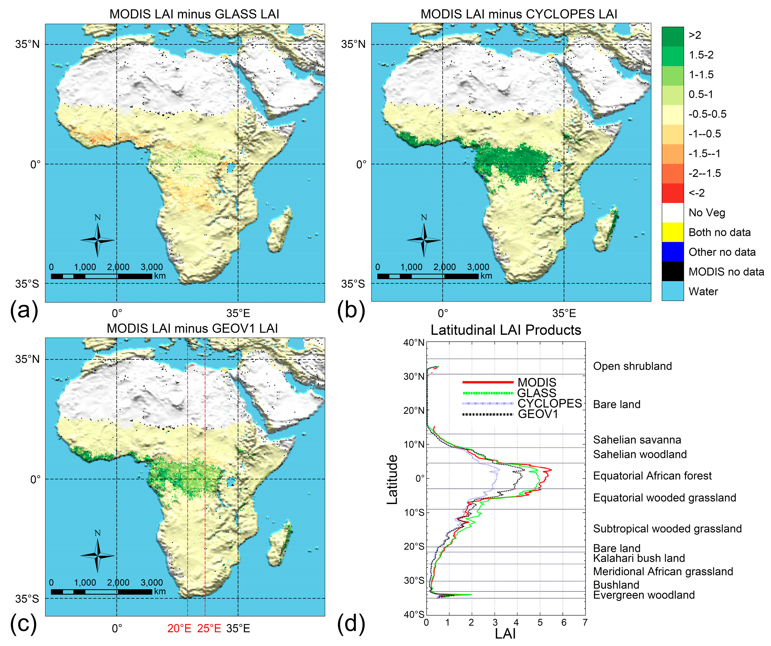
4.2.2. Continental Consistency

The African continent, which is divided by the equator, was selected to assess the spatial consistency among LAIs from the four products at the continental scale. Figure 5a–c indicates that the best spatial agreement is achieved between MODIS and GLASS, with LAI differences ranging within ±1. A significant underestimation (>2 LAI unit) is found over the central Africa forests in the case of CYCLOPES. This is somewhat alleviated in GEOV1. Missing data are not found in these annual average datasets, except in the case of MODIS near the boundaries of water bodies or barren areas.

Figure 5d displays LAIs from MODIS, GLASS, CYCLOPES and GEOV1 along the transect within the longitude bands between 20° E and 25° E. The most obvious inconsistency is seen in equatorial forests, where LAI differences can reach one unit. CYCLOPES underestimates other products in these regions with unrealistically low LAI values. The products agree better over open shrublands and savannas. GEOV1 and CYCLOPES also show good consistency over the subtropical wooded grasslands, while GLASS overestimates them significantly. Two product groups (MODIS-GLASS and GEOV1-CYCLOPES) can be distinguished clearly over the bush lands and meridional African grasslands. This suggests that the input data sources to the algorithms play an important role in affecting the variation and magnitude of LAI/FPAR retrievals.

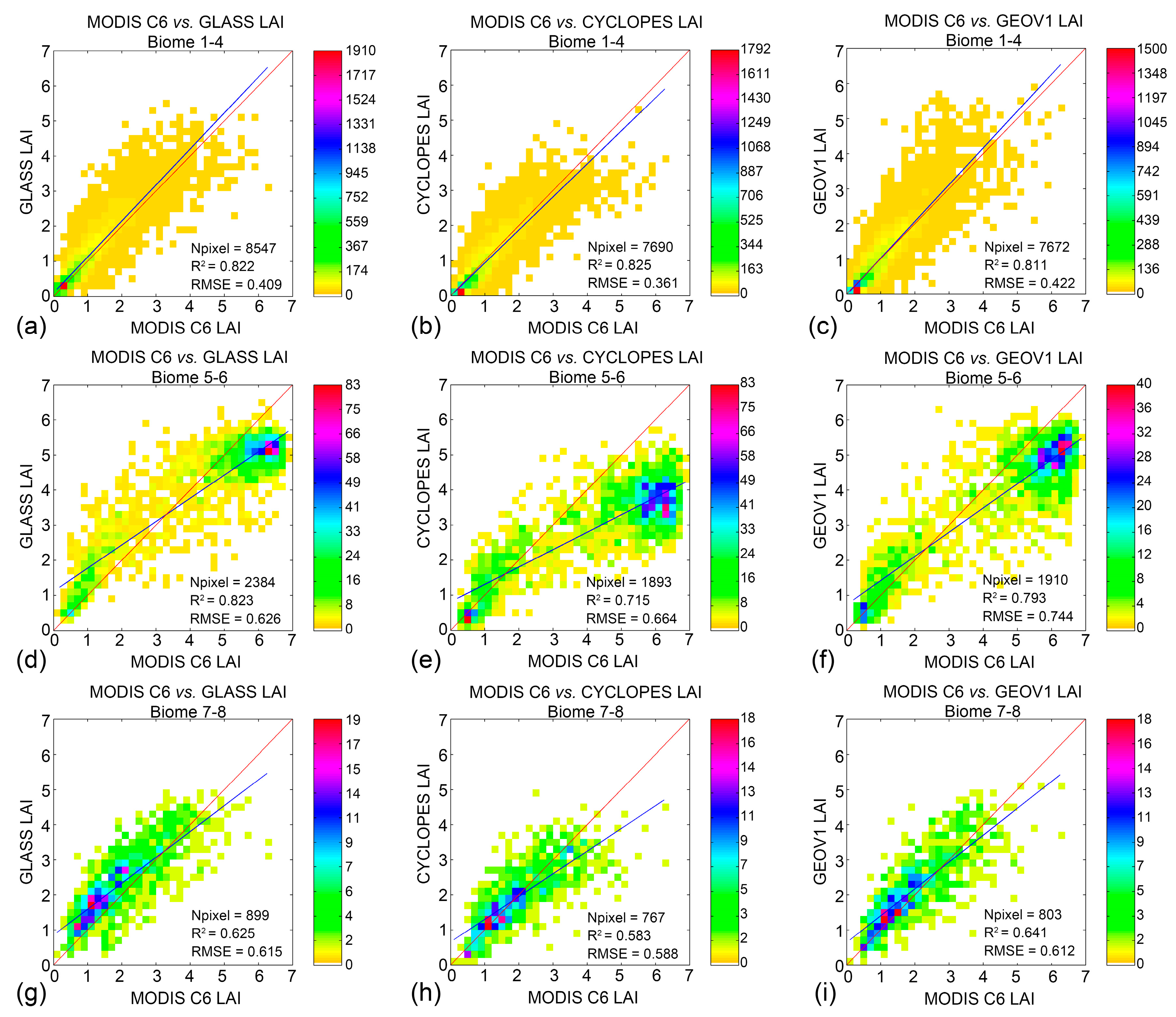
4.2.3. Comparison over BELMANIP Sites

Density scatter plots of monthly LAI extracted from the four products over BELMANIP2.1 sites during the period from 2001–2005 are shown in Figure 6. Results for three broad vegetation classes (non-forest, broadleaf forests and needleleaf forests) are shown separately in

Table 4. Statistics of the intercomparisons among four LAI/FPAR products over BELMANIP sites during 2001–2005. Eight biome types are grouped into three broad categories (1–4: non-forest; 5–6: broadleaf forests; 7–8: needleleaf forests). R², RMSE and regression equations are provided.

Biomes		MODIS-GLASS	MODIS-CYCLOPES	MODIS-GEOV1	GLASS-CYCLOPES	GLASS-GEOV1	CYCLOPES-GEOV1
LAI	1–4	0.82/0.41/y = 1.03x + 0.10	0.83/0.36/y = 0.94x − 0.01	0.81/0.42/y = 1.05x − 0.03	0.86/0.34/y = 0.85x − 0.03	0.83/0.41/y = 0.94x − 0.06	0.95/0.23/y = 1.09x − 0.01
	5–6	0.82/0.63/y = 0.66x + 1.11	0.72/0.66/y = 0.50x + 0.81	0.79/0.74/y = 0.69x + 0.73	0.77/0.59/y = 0.69x + 0.17	0.80/0.72/y = 1.03x + 0.10	0.89/0.55/y = 1.26x + 0.05
	7–8	0.63/0.62/y = 0.74x + 0.86	0.58/0.59/y = 0.65x + 0.66	0.64/0.61/y = 0.76x + 0.64	0.65/0.57/y = 0.73x + 0.25	0.70/0.60/y = 0.86x + 0.16	0.85/0.43/y = 1.07x + 0.06
	All	0.90/0.53/y = 0.83x + 0.31	0.83/0.53/y = 0.64x + 0.26	0.88/0.56/y = 0.82x + 0.19	0.89/0.44/y = 0.74x + 0.06	0.91/0.50/y = 0.95x − 0.06	0.95/0.36/y = 1.23x − 0.07
FPAR	1–4	N/A	0.89/0.07/y = 1.04x − 0.08	0.88/0.08/y = 1.17x − 0.08	N/A	N/A	0.97/0.04/y = 1.12x + 0.01
	5–6	N/A	0.75/0.08/y = 0.77x + 0.07	0.80/0.08/y = 0.88x + 0.09	N/A	N/A	0.93/0.05/y = 1.06x + 0.06
	7–8	N/A	0.53/0.10/y = 0.75x + 0.09	0.59/0.10/y = 0.82x + 0.12	N/A	N/A	0.82/0.07/y = 0.93x + 0.11
	All	N/A	0.91/0.08/y = 0.95x − 0.05	0.91/0.09/y = 1.08x − 0.05	N/A	N/A	0.97/0.05/y = 1.12x + 0.01

.

Figure 6a–c shows comparisons over non-forest sites where the best agreements between any two products are observed. LAI values over these sites range from 0–2. Within this range, reflectances are not saturated, and the respective algorithms perform well. Regression lines are close to the 1:1 line with R² better than 0.81 and RMSE smaller than 0.42 (LAI) and 0.08 (FPAR) in all cases. This result satisfies the target accuracy (±0.5 LAI unit) expected by the Global Climate Observation System (GCOS) [31]. MODIS seems to underestimate GLASS and GEOV1, but slightly overestimates CYCLOPES. Minimum bias (R² = 0.95, RMSE = 0.23) is achieved between CYCLOPES and GEOV1.

Figure 6d–f shows the case for broadleaf forests where the largest discrepancies are observed. The largest RMSE (0.74) is seen in the MODIS versus GEOV1 comparison and the smallest (0.55) between CYCLOPES and GEOV1. The plots show an interesting pattern where the data are in two clusters, which may be due to the monthly temporal resolution in this analysis resulting in missing some parts of the seasonality of deciduous forests. MODIS tends to underestimate in the low-LAI domain and overestimate in the high-LAI domain, relative to other products.

Similar comparisons over needleleaf forests are shown in Figure 6g–i. The total number of observations is less than 900, and this may result in additional uncertainties. CYCLOPES and GEOV1 agree well in terms of R² (0.85 for LAI and 0.82 for FPAR) and minimum RMSE (0.43 for LAI and 0.07 for FPAR). The discrepancies between MODIS and other products are similar with R² around 0.6. A slight underestimation can be noticed for MODIS at low values, especially compared to GLASS.

When considering all biome types, the RMSE of LAI (FPAR) derived from any two products ranges from 0.36 (0.05)–0.56 (0.09). The sequence from best to worst agreement is: CYCLOPES-GEOV1, GLASS-CYCLOPES, GLASS-GEOV1, MODIS-GLASS, MODIS-CYCLOPES and MODIS-GEOV1.

4.2.4. Temporal Comparison

Temporal Continuity

In the time series of LAI/FPAR products, there would be some gaps (missing data) mainly due to cloud or snow contamination, poor atmospheric conditions or technical problems, which will limit their use in land surface models [7,8]. Here, we define the “annual missing data rate” as the percent of months without valid data during the whole year. It represents the fraction in time of missing data. Note that the quality control applied for different products could be an important factor affecting this criterion.

The four lines in the upper part of Figure 7 represent variations of missing data for MODIS, GLASS, CYCLOPES and GEOV1 through four years (2001–2004). Missing data are also indicated by gaps in the LAI/FPAR time series. The missing data rate ranges from 0%–40% (five months of no data) over the seven sites. Most missing data are in the winter season, which is related to cloudiness, snow and poor atmospheric conditions, especially for high latitude sites. Sites with shrubs, broadleaf crops, savannas and broadleaf forests show low missing data rates (<20%). The four products exhibit different behaviors over different sites, and no clear conclusions can be drawn. GLASS tends to have low missing data, which may be due to a gap-filling procedure in its algorithm. GEOV1 shows a similar missing data rate as CYCLOPES, which may be expected, as both products use the same preprocessed SPOT-VGT data. MODIS shows a moderate missing data rate for most sites, which is not in agreement with some other studies [8]. This may be because our study is based on a normalized monthly temporal step instead of the native temporal resolution of each product. In addition, quality control procedures applied to the different products also affect the number of valid data in the time series.

Temporal Consistency

The consistency of the temporal trajectory of each product over seven validation sites for the period from 2001–2004 is discussed in this section (Figure 7). All available ground measurements are plotted in these figures as a reference. Statistics (R² and RMSE) of these temporal comparisons are given in

Table 5. Statistics of temporal comparisons among four LAI/FPAR products over seven validation sites during 2001–2004. R² and RMSE are provided. Values out of and in blankets are for LAI and FPAR, respectively.

Site and Biome	MODIS-GLASS		MODIS-CYCLOPES		MODIS-GEOV1		GLASS-CYCLOPES		GLASS-GEOV1		CYCLOPES-GEOV1
	R2	RMSE	R2	RMSE	R2	RMSE	R2	RMSE	R2	RMSE	R2	RMSE
#78:B1	0.96	0.14	0.91(0.91)	0.17(0.09)	0.94(0.93)	0.15(0.07)	0.95	0.16	0.94	0.17	0.97(0.97)	0.10(0.05)
#88:B2	0.65	0.12	0.61(0.69)	0.20(0.11)	0.76(0.60)	0.16(0.10)	0.82	0.11	0.87	0.10	0.86(0.88)	0.10(0.06)
#1:B3	0.98	0.66	0.96(0.96)	0.62(0.08)	0.93(0.94)	0.95(0.10)	0.98	0.20	0.94	0.39	0.95(0.98)	0.45(0.05)
#103:B4	0.84	0.21	0.75(0.72)	0.42(0.10)	0.79(0.80)	0.40(0.06)	0.89	0.42	0.90	0.38	0.96(0.95)	0.1(0.06)
#96:B5	0.08	1.01	0.01(0.00)	2.56(0.19)	0.00(0.00)	1.70(0.08)	0.53	1.61	0.45	0.76	0.81(0.80)	1.01(0.13)
#58:B6	0.54	1.12	0.89(0.66)	0.57(0.12)	0.86(0.66)	0.56(0.08)	0.50	1.15	0.48	1.12	0.91(0.76)	0.74(0.10)
#68:B7	0.89	0.72	0.45(0.34)	0.69(0.12)	0.74(0.64)	0.68(0.06)	0.57	0.81	0.83	0.53	0.76(0.58)	0.74(0.11)

.

The four products show smooth and consistent annual variations in the case of the Zhangbei grassland site in China, with some gaps in the winter season that may be due to snow contamination (Figure 7a). LAI and FPAR exhibit bell-shaped profiles, with LAI ranging from almost zero in winter to more than one in summer and FPAR ranging from 0–0.5. CYCLOPES displays systematic underestimation, as documented previously [8]. MODIS C6 is still found to systematically overestimate FPAR in sparse canopies, a problem also seen in C5 [15].

All of the products achieve good temporal continuity in shrubs (Figure 7b). LAI and FPAR are relatively low, as rainfall is limited over this site. GLASS, CYCLOPES and GEOV1 agree well, especially at low values of LAI and FPAR. MODIS shows a generally different seasonal profile, which may be realistic [32]. We find that all products overestimate both LAI and FPAR ground measurements.

Figure 7c shows the temporal variations of broadleaf crops over the AGRO site. This site shows similar temporal variations as the Zhangbei site, being about the same latitude, but there are differences in magnitude. LAI and FPAR values can reach four and 0.8, respectively. GLASS, CYCLOPE and GEOV1 agree with each other well, especially in the years 2001 and 2002. However, MODIS shows an underestimation for LAI during the growing season and overestimation of FPAR in the winter season. The LAI difference between MODIS and GEOV1 is larger than two in 2003.

The savanna site shows a different pattern of seasonality as compared to grasses, shrubs and broadleaf crops (Figure 7d). The seasonality is relatively damped with LAI values ranging from 0.5–2. The four products show similar LAI/FAPR variations and agree with ground measurements well. MODIS has no missing data during the four years.

The consistency between the four products is the worst over the EBF site (Figure 7e). This site is in Budongo rainforests where the dry season only spans from December–February and June/July. The field campaign conducted in October/November 2005 reported that LAI varies between 5.19 and 10.47 [33]. However, no clear seasonality is captured by any of the products from LAI or FPAR with high missing data rate. Similar results were reported by other studies [7,8]. This can be explained by the poor quality of satellite products due to cloud contamination and poor atmospheric conditions. The ground measurement in 2003 shows good agreement with MODIS LAI.

Figure 7f shows the case for a DBF site located in the northern high latitude. GEOV1 and MODIS agree best and are the closest to ground measurements for both LAI and FPAR in 2002. As expected, CYCLOPES underestimates all of the other products because of a lack of correction for clumping effects. Compared to others, GLASS shows artifacts related to smoothing and/or gap-filling procedures.

The four products show very similar seasonality over the ENF site (Figure 7g). LAI at this site ranges from 1–5. Thus, saturation effects are prominently seen in CYCLOPES. The MODIS profiles are noisier due to the sensitivity of retrievals to noise in reflectances at high values of LAI [7]. All products generally agree with available ground measurements. We note that CYCLOPES is closer to effective LAI measurements that is smaller than true LAI due to clumping effects.

Table 5 shows the statistical results from temporal comparisons among the four LAI/FPAR products over the seven sites during 2001–2004. R² and RMSE are provided as indicators of consistency. The best agreement among four products is seen in the grasses (B1) and broadleaf crops (B3) sites, with R² better than 0.9. The agreement between MODIS and other products is least over the EBF (B5) site. Over this site, the RMSE between MODIS and CYCLOPES is 2.56 and 0.19 for LAI and FPAR, respectively. Lager RMSE values over densely-vegetated sites (B4–B7) are observed between CYCLOPES and other products, which is due to premature saturation in the CYCLOPES algorithm [8]. Overall, MODIS agrees best with GLASS, and CYCLOPES agrees best with GEOV1. This is not surprising, as these pairs of products have the same underlying reflectances.

4.3. Evaluation with Climate Variables

Spatial and temporal variations of biophysical variables can be assessed for consistency with changes observed in meteorological fields. Several studies have focused on the relationship between the temporal variation of LAI and climate variables that govern plant growth in particular regions. From these studies, obvious correlation between LAI and precipitation in tropical regions and temperature in high latitudes regions have been reported [7,11,34,35]. In this section, we discuss the correlation between C6 LAI and temperature in northern latitudes and precipitation in some ENSO (El Niño-Southern Oscillation)-affected regions.

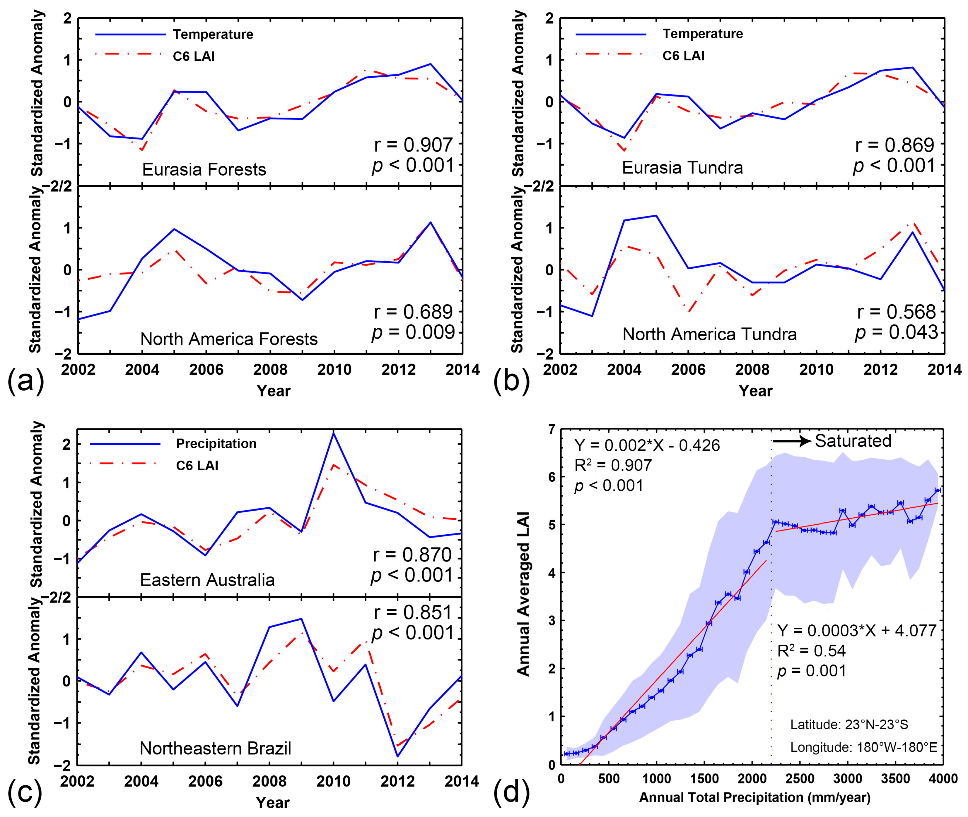
4.3.1. LAI Variation with Surface Temperature

Here, we present interannual variations of C6 LAI and assess their correlation to surface temperature, which can be helpful in verifying the variations in the LAI product. The spatial (60° N–90° N) and temporal (April and May) averages of standardized anomalies of LAI and surface temperature are shown in Figure 8a,b for forests and tundra, respectively. The greening trend in Eurasia was reported to be more obvious than in North America [36]. Therefore, the analysis was done separately for these two continents.

The anomaly time series of surface temperature and LAI correlate remarkably well, especially in Eurasian forests with a 0.907 correlation coefficient. The linkage is stronger in Eurasia than in North America. This is because North American boreal forests have experienced declining photosynthetic activity due to recent warming-induced drought, wild fires and pest infestations [37]. Our results also indicate that correlations in tundra are considerably weaker than in forests. This could be due to fewer valid data over tundra resulting from poor Sun-sensor geometry and illumination conditions. Nevertheless, we observe a slight warming and greening trend in Eurasian forests (p = 0.033 in a Mann–Kendall trend test [38]). However, no statistically-significant trend is found in tundra or North American forests (p > 0.1), which agrees with [11,35].

4.3.2. LAI Variation with Precipitation

The standardized anomalies of thirteen years of LAI and precipitation in two semiarid regions are shown in Figure 8c. Significant coherence between LAI and rainfall anomalies are found in both eastern Australia (r = 0.87, p < 0.001) and northeastern Brazil (r = 0.851, p < 0.001). We do not find particular directional changes in precipitation or vegetation greenness in these two regions during the period of our study. However, the high precipitation events leading to damaging Australian floods in 2010–2011 [39] are obvious with a peak in both precipitation and LAI variations. Moreover, we notice a severe drought with corresponding vegetation browning occurring in northeastern Brazil in 2012, which has been confirmed in [40].

Figure 8d shows the correlation between annual averaged LAI and annual total precipitation in the tropical latitudes (23° S–23° N). Note that this analysis was not for a specific year, but for the average of thirteen years. The precipitation range (0–4000 mm/year) was divided into 40 intervals. The mean and standard deviation of annual averaged LAI in each of the 40 precipitation bins were first computed for each of the thirteen years and then averaged over the thirteen years. We find a highly significant correlation (R² = 0.97, p < 0.001) between the two variables when precipitation is less than 2200 mm/year from where this relationship turns to saturated. Large standard deviations of LAI within each precipitation interval indicate the role of other factors in governing plant growth [35].

5. Conclusions

The objective of this paper is to evaluate the newly-released MODIS LAI/FPAR C6 product (MOD15A2H). This is achieved comprehensively through three independent approaches: validation with ground measurements, intercomparison with other satellite products and comparison with climate variables. Fifty four true LAI, 82 effective LAI and 45 FPAR ground measurements with high reliability extracted from 113 sites were used to validate the C6 and C5 LAI/FPAR products. The results showed that MODIS LAI is closer to true LAI, rather than effective LAI, due to the clumping correction in the algorithm. We found that MODIS C6 performed considerably better than C5 in comparisons to true LAI measurements. The RMSE decreased from 0.80 down to 0.66, which is close to the target accuracy (±0.5) as required by the GCOS. Both C5 and C6 showed an overestimation of FPAR over sparsely-vegetated areas, as noted previously in other studies.

Intercomparisons with three other satellite products (GLASS, CYCLOPES and GEOV1) were carried out at the site, continental and global scales to investigate the differences. The four products showed similar spatial distributions of LAI and FPAR in both January and July. MODIS and GLASS (CYCLOPES and GEOV1) were found to achieve the best agreement, most likely because the surface reflectances used as inputs to the respective algorithms were acquired from the same instrument. CYCLOPES underestimated LAI and FPAR systematically due to the lack of correction for clumping effects and premature saturation. Temporal comparisons for the 2001–2004 period indicated that the products properly captured the seasonality of different biomes, except in EBF, where the poor quality of satellite products resulted in erratic and unrealistic seasonal profiles. The four products showed different performances at different sites in terms of missing data, and no clear conclusion could be drawn.

To further imbue confidence in the LAI product, we assessed correlations between the variations of satellite-derived LAI and station-measured temperature and precipitation data over a thirteen year period. Statistically-significant agreements between these data series indicated that the interannual variations in LAI are not an artifact of remote sensing data or the algorithm.

The research presented here is critical for the further understanding and proper use of C6 LAI/FPAR products in land surface models. Furthermore, the validation and intercomparison approaches presented in this work can be used for the evaluation of similar products in the future.

References

1. Sellers, P.J.; Dickinson, R.E.; Randall, D.A.; Betts, A.K.; Hall, F.G.; Berry, J.A.; Collatz, G.J.; Denning, A.S.; Mooney, H.A.; Nobre, C.A. Modeling the exchanges of energy, water, and carbon between continents and the atmosphere. Science 1997, 275, 502–509. [Google Scholar] [CrossRef]
2. Myneni, R.B.; Smith, G.R.; Lotsch, A.; Friedl, M.; Morisette, J.T.; Votava, P.Ô.N.R.; Running, S.W.; Hoffman, S.; Knyazikhin, Y.; Privette, J.L.; et al. Global products of vegetation leaf area and fraction absorbed PAR from year one of MODIS data. Remote Sens. Environ. 2002, 83, 214–231. [Google Scholar] [CrossRef]
3. Xiao, Z.; Liang, S.; Wang, J.; Chen, P.; Yin, X.; Zhang, L.; Song, J. Use of general regression neural networks for generating the GLASS leaf area index product from time-series MODIS surface reflectance. IEEE Trans. Geosci. Remote Sens. 2014, 52, 209–223. [Google Scholar] [CrossRef]
4. Baret, F.; Weiss, M.; Lacaze, R.; Camacho, F.; Makhmara, H.; Pacholcyzk, P.; Smets, B. GEOV1: LAI and FAPAR essential climate variables and FCOVER global time series capitalizing over existing products. Part1: Principles of development and production. Remote Sens. Environ. 2013, 137, 299–309. [Google Scholar] [CrossRef]
5. Yan, K.; Park, T.; Yan, G.; Chen, C.; Yang, B.; Liu, Z.; Nemani, R.; Knyazikhin, Y.; Myneni, R. Evaluation of MODIS LAI/FPAR product Collection 6. Part 1: Consistency and improvements. Remote Sens. 2016, 8, 359. [Google Scholar] [CrossRef]
6. Fang, H.; Wei, S.; Liang, S. Validation of MODIS and CYCLOPES LAI products using global field measurement data. Remote Sens. Environ. 2012, 119, 43–54. [Google Scholar] [CrossRef]
7. Garrigues, S.; Lacaze, R.; Baret, F.; Morisette, J.T.; Weiss, M.; Nickeson, J.E.; Fernandes, R.; Plummer, S.; Shabanov, N.V.; Myneni, R.B.; et al. Validation and intercomparison of global Leaf Area Index products derived from remote sensing data. J. Geophys. Res. 2008, 113. [Google Scholar] [CrossRef]
8. Camacho, F.; Cernicharo, J.; Lacaze, R.; Baret, F.; Weiss, M. GEOV1: LAI, FAPAR essential climate variables and FCOVER global time series capitalizing over existing products. Part 2: Validation and intercomparison with reference products. Remote Sens. Environ. 2013, 137, 310–329. [Google Scholar] [CrossRef]
9. Yang, W.; Tan, B.; Huang, D.; Rautiainen, M.; Shabanov, N.V.; Wang, Y.; Privette, J.L.; Huemmrich, K.F.; Fensholt, R.; Sandholt, I.; et al. MODIS leaf area index products: From validation to algorithm improvement. IEEE Trans. Geosci. Remote Sens. 2006, 44, 1885–1898. [Google Scholar] [CrossRef]
10. Fang, H.; Jiang, C.; Li, W.; Wei, S.; Baret, F.; Chen, J.M.; Garcia-Haro, J.; Liang, S.; Liu, R.; Myneni, R.B.; et al. Characterization and intercomparison of global moderate resolution leaf area index (LAI) products: Analysis of climatologies and theoretical uncertainties. J. Geophys. Res. Biogeosci. 2013, 118, 529–548. [Google Scholar] [CrossRef]
11. Ganguly, S.; Samanta, A.; Schull, M.A.; Shabanov, N.V.; Milesi, C.; Nemani, R.R.; Knyazikhin, Y.; Myneni, R.B. Generating vegetation leaf area index Earth system data record from multiple sensors. Part 2: Implementation, analysis and validation. Remote Sens. Environ. 2008, 112, 4318–4332. [Google Scholar] [CrossRef]
12. Steinberg, D.C.; Goetz, S.J.; Hyer, E.J. Validation of MODIS F/sub PAR/products in boreal forests of Alaska. IEEE Trans. Geosci. Remote Sens. 2006, 44, 1818–1828. [Google Scholar] [CrossRef]
13. Tan, B.; Hu, J.; Zhang, P.; Huang, D.; Shabanov, N.; Weiss, M.; Knyazikhin, Y.; Myneni, R.B. Validation of Moderate Resolution Imaging Spectroradiometer leaf area index product in croplands of Alpilles, France. J. Geophys. Res. Atmos. 2005, 110. [Google Scholar] [CrossRef]
14. Knyazikhin, Y.; Glassy, J.; Privette, J.L.; Tian, Y.; Lotsch, A.; Zhang, Y.; Wang, Y.; Morisette, J.T.; Votava, P.; Myneni, R.B. MODIS Leaf Area Index (LAI) and Fraction of Photosynthetically Active Radiation Absorbed by Vegetation (FPAR) Product (MOD15) Algorithm Theoretical Basis Document; Theoretical Basis Document; NASA Goddard Space Flight Center: Greenbelt, MD, USA, 1999; p. 20771. [Google Scholar]
15. Majasalmi, T.; Rautiainen, M.; Stenberg, P.; Manninen, T. Validation of MODIS and GEOV1 fPAR Products in a Boreal Forest Site in Finland. Remote Sens. 2015, 7, 1359–1379. [Google Scholar] [CrossRef]
16. Liang, S.; Zhao, X.; Liu, S.; Yuan, W.; Cheng, X.; Xiao, Z.; Zhang, X.; Liu, Q.; Cheng, J.; Tang, H. A long-term Global LAnd Surface Satellite (GLASS) data-set for environmental studies. Int. J. Digit. Earth 2013, 6, 5–33. [Google Scholar] [CrossRef]
17. Baret, F.; Hagolle, O.; Geiger, B.; Bicheron, P.; Miras, B.; Huc, M.; Berthelot, B.; Niño, F.; Weiss, M.; Samain, O. LAI, fAPAR and fCover CYCLOPES global products derived from VEGETATION: Part 1: Principles of the algorithm. Remote Sens. Environ. 2007, 110, 275–286. [Google Scholar] [CrossRef] [Green Version]
18. Weiss, M.; Baret, F.; Garrigues, S.; Lacaze, R. LAI and fAPAR CYCLOPES global products derived from VEGETATION. Part 2: Validation and comparison with MODIS collection 4 products. Remote Sens. Environ. 2007, 110, 317–331. [Google Scholar] [CrossRef]
19. Jacquemoud, S.; Verhoef, W.; Baret, F.; Bacour, C.; Zarco-Tejada, P.J.; Asner, G.P.; François, C.; Ustin, S.L. PROSPECT+ SAIL models: A review of use for vegetation characterization. Remote Sens. Environ. 2009, 113, S56–S66. [Google Scholar] [CrossRef]
20. Morisette, J.T.; Baret, F.; Privette, J.L.; Myneni, R.B.; Nickeson, J.E.; Garrigues, S.; Shabanov, N.V.; Weiss, M.; Fernandes, R.; Leblanc, S.G. Validation of global moderate-resolution LAI products: A framework proposed within the CEOS land product validation subgroup. IEEE Trans. Geosci. Remote Sens. 2006, 44, 1804. [Google Scholar] [CrossRef]
21. Baret, F.; Morissette, J.T.; Fernandes, R.A.; Champeaux, J.L.; Myneni, R.B.; Chen, J.; Plummer, S.; Weiss, M.; Bacour, C.; Garrigues, S.; et al. Evaluation of the representativeness of networks of sites for the global validation and intercomparison of land biophysical products: Proposition of the CEOS-BELMANIP. IEEE Trans. Geosci. Remote Sens. 2006, 44, 1794–1803. [Google Scholar] [CrossRef]
22. Harris, I.; Jones, P.D.; Osborn, T.J.; Lister, D.H. Updated high-resolution grids of monthly climatic observations—The CRU TS3. 10 Dataset. Int. J. Climatol. 2014, 34, 623–642. [Google Scholar] [CrossRef] [Green Version]
23. Hu, R.; Yan, G.; Mu, X.; Luo, J. Indirect measurement of leaf area index on the basis of path length distribution. Remote Sens. Environ. 2014, 155, 239–247. [Google Scholar] [CrossRef]
24. Chen, J.M.; Cihlar, J. Quantifying the effect of canopy architecture on optical measurements of leaf area index using two gap size analysis methods. IEEE Trans. Geosci. Remote Sens. 1995, 33, 777–787. [Google Scholar] [CrossRef]
25. Yan, G.; Hu, R.; Wang, Y.; Ren, H.; Song, W.; Qi, J.; Chen, L. Scale Effect in Indirect Measurement of Leaf Area Index. IEEE Trans. Geosci. Remote Sens 2016. [Google Scholar] [CrossRef]
26. Martínez, B.; García-Haro, F.J.; Camacho-de Coca, F. Derivation of high-resolution leaf area index maps in support of validation activities: Application to the cropland Barrax site. Agric. For. Meteorol. 2009, 149, 130–145. [Google Scholar] [CrossRef]
27. Fernandes, R.; Butson, C.; Leblanc, S.; Latifovic, R. Landsat-5 TM and Landsat-7 ETM+ based accuracy assessment of leaf area index products for Canada derived from SPOT-4 VEGETATION data. Can. J. Remote Sens. 2003, 29, 241–258. [Google Scholar] [CrossRef]
28. Mayr, M.; Samimi, C. Comparing the dry season in-situ Leaf Area Index (LAI) derived from high-resolution rapideye imagery with MODIS LAI in a namibian Savanna. Remote Sens. 2015, 7, 4834–4857. [Google Scholar] [CrossRef]
29. Stenberg, P. Correcting LAI-2000 estimates for the clumping of needles in shoots of conifers. Agric. For. Meteorol. 1996, 79, 1–8. [Google Scholar] [CrossRef]
30. Rajeevan, M.; Bhate, J.; Kale, J.D.; Lal, B. High resolution daily gridded rainfall data for the Indian region: Analysis of break and active monsoon spells. Curr Sci. India 2006, 91, 296–306. [Google Scholar]
31. GCOS. Systematic Observation Requirements for Satellite-Based Products for Climate: Supplemental Details to the Satellite-Based Component of the “Implementation Plan for the Global Observing System for Climate in Support of the UNFCCC”; GCOS: Singapore, Singapore, 2006. [Google Scholar]
32. Elmore, A.J.; Guinn, S.M.; Minsley, B.J.; Richardson, A.D. Landscape controls on the timing of spring, autumn, and growing season length in mid-Atlantic forests. Glob. Chang. Biol. 2012, 18, 656–674. [Google Scholar] [CrossRef]
33. Kraus, T.; Schmidt, M.; Dech, S.W.; Samimi, C. The potential of optical high resolution data for the assessment of leaf area index in East African rainforest ecosystems. Int. J. Remote Sens. 2009, 30, 5039–5059. [Google Scholar] [CrossRef]
34. Buermann, W. Analysis of a multiyear global vegetation leaf area index data set. J. Geophys. Res. Atmos. 2002, 107. [Google Scholar] [CrossRef]
35. Zhu, Z.; Bi, J.; Pan, Y.; Ganguly, S.; Anav, A.; Xu, L.; Samanta, A.; Piao, S.; Nemani, R.; Myneni, R. Global data sets of vegetation Leaf Area Index (LAI)3g and Fraction of Photosynthetically Active Radiation (FPAR)3g derived from Global Inventory Modeling and Mapping Studies (GIMMS) Normalized Difference Vegetation Index (NDVI3g) for the period 1981 to 2011. Remote Sen. 2013, 5, 927–948. [Google Scholar]
36. Zhou, L.; Tucker, C.J.; Kaufmann, R.K.; Slayback, D.; Shabanov, N.V.; Myneni, R.B. Variations in northern vegetation activity inferred from satellite data of vegetation index during 1981 to 1999. J. Geophys. Res. Atmos. 2001, 106, 20069–20083. [Google Scholar] [CrossRef]
37. Goetz, S.J.; Bunn, A.G.; Fiske, G.J.; Houghton, R.A. Satellite-observed photosynthetic trends across boreal North America associated with climate and fire disturbance. Proc. Natl. Acad. Sci. USA 2005, 102, 13521–13525. [Google Scholar] [CrossRef] [PubMed]
38. Yue, S.; Pilon, P.; Cavadias, G. Power of the Mann—Kendall and Spearman’s rho tests for detecting monotonic trends in hydrological series. J. Hydrol. 2002, 259, 254–271. [Google Scholar] [CrossRef]
39. Boening, C.; Willis, J.K.; Landerer, F.W.; Nerem, R.S.; Fasullo, J. The 2011 La Niña: So strong, the oceans fell. Geophys. Res. Lett. 2012, 39. [Google Scholar] [CrossRef]
40. Marengo, J.A.; Alves, L.M.; Soares, W.R.; Rodriguez, D.A.; Camargo, H.; Riveros, M.P.; Pabló, A.D. Two contrasting severe seasonal extremes in tropical South America in 2012: Flood in Amazonia and drought in northeast Brazil. J. Clim. 2013, 26, 9137–9154. [Google Scholar] [CrossRef]
Figure 1. Biome type distribution within each 3 km × 3 km validation site based on the 500-m resolution MODIS C5 land cover product. The bottom part of the plot shows biome types and the corresponding proportion of coverage within each site. EBF, DBF, ENF and DNF stand for “Evergreen Broadleaf Forest”, “Deciduous Broadleaf Forest”, “Evergreen Needleleaf Forest” and “Deciduous Needleleaf Forest”, respectively. The top part of the plot shows the biome type information entropy of each site calculated using Equation (5). Zero means there is only one biome type in the site or the site is a homorganic site. A larger entropy value means larger heterogeneity.
Remotesensing 08 00460 g001
Figure 2. Comparisons between ground measured LAI (a,b) and FPAR (c,d) with MODIS C5 (left panels) and C6 (right panels) retrievals. Fifty four true LAI, 82 effective LAI and 45 FPAR measurements are used here. The 3 km × 3 km sites dominated by different biome types are depicted by different colors. Circles (triangles) in (a) and (b) represent ground LAI measurements corrected (not corrected) for clumping.
Remotesensing 08 00460 g002
Figure 3. Global distribution of absolute differences between (a) MODIS and GLASS LAI; (b) MODIS and CYCLOPES LAI; (c) MODIS and GEOV1 LAI; (d) MODIS and CYCLOPES FPAR; and (e) MODIS and GEOV1 FPAR in July 2001. The spatial resolution is 0.25 degrees.
Remotesensing 08 00460 g003aRemotesensing 08 00460 g003b
Figure 4. Histograms of global LAI (a,b) and FPAR values (c,d) from four products analyzed in this study during the months of January and July of 2001. The frequency is given as the percentage of the total number of global vegetated pixels. Global mean LAI values are depicted by vertical lines. The bins used for LAI and FPAR are 0.25 and 0.05, respectively.
Remotesensing 08 00460 g004
Figure 5. Comparisons of annual averaged LAI from the MODIS, GLASS, CYCLOPES and GEOV1 products over Africa in 2001. (ac) Absolute differences between MODIS C6 and GLASS, CYCLOPES and GEOV1; (d) LAI from four products along the transect in Africa between 20° E and 25° E.
Remotesensing 08 00460 g005
Figure 6. Density scatter plots of monthly MODIS LAI and three other LAI products (left: GLASS; middle: CYCLOPES; right: GEOV1) over BELMANIP sites during the time period from 2001–2005. The plots show a correlation between MODIS and other products for non-forest ((ac) Biomes 1–4) in the first row, broadleaf forests ((df) Biomes 5 and 6) in the second row and needle leaf forests ((gi) Biomes 7 and 8) in the third row. The red lines and blue lines are the 1:1 lines and regression lines derived from the scatter plots, respectively.
Remotesensing 08 00460 g006
Figure 7. Temporal comparisons of LAI and FPAR among MODIS C6, GLASS, CYCLOPES and GEOV1 products over seven validation sites. Monthly averaged LAI and FAPR values for the time period from 2001–2004 are shown here. Circles, stars and triangles represent ground measurements of true LAI, effective LAI and FPAR, respectively. The four lines plotted at the top represent variations in missing data in each year. (a) Grasses; (b) shrubs; (c) broadleaf crops; (d) savanna; (e) EBF; (f) DBF; and (g) ENF.
Remotesensing 08 00460 g007aRemotesensing 08 00460 g007b
Figure 8. Evaluation of the MODIS LAI C6 product with temperature in the northern latitudes and precipitation in the ENSO-affected regions. (a) Temporal variations of the standardized anomalies of the growing season start period (April and May) averages of LAI and temperature for forest pixels in the northern latitudes; (b) same as (a), but for tundra pixels; (c) temporal variations of the standardized anomalies of annual summed LAI and precipitation in eastern Australia (20° S–40° S, 145° E–155° E) and northeastern Brazil (3° S–12° S, 35° W–45° W); (d) correlation between annual averaged LAI and annual total precipitation in the tropical latitudes (23° S–23° N). Standard deviations of LAIs and precipitations are denoted by blue shadow and horizontal error bars, respectively.
Remotesensing 08 00460 g008