Estimation of Daily Solar Radiation Budget at Kilometer Resolution over the Tibetan Plateau by Integrating MODIS Data Products and a DEM

Abstract

Considering large and complex areas like the Tibetan Plateau, an analysis of the spatial distribution of the solar radiative budget over time not only requires the use of satellite remote sensing data, but also of an algorithm that accounts for strong variations of topography. Therefore, this research aims at developing a method to produce time series of solar radiative fluxes at high temporal and spatial resolution based on observed surface and atmosphere properties and topography. The objective is to account for the heterogeneity of the land surface using multiple land surface and atmospheric MODIS data products combined with a digital elevation model to produce estimations daily at the kilometric level. The developed approach led to the production of a three-year time series (2008–2010) of daily solar radiation budget at one kilometer spatial resolution across the Tibetan Plateau. The validation showed that the main improvement from the proposed method is a higher spatial and temporal resolution as compared to existing products. However, even if the solar radiation estimates are satisfying on clear sky conditions, the algorithm is less reliable under cloudy sky condition and the albedo product used here has a too coarse temporal resolution and is not accurate enough over rugged terrain.

1. Introduction

Radiation fluxes at the Earth’s surface drive processes like evaporation, photosynthesis, and heating of soil and air. Therefore, they are important variables in vegetation dynamics and climate change modelling [1,2], as well as key indicators of drought [3]. The solar radiation budget, also called net solar radiation, is defined as the difference between incident and reflected shortwave radiative fluxes at the Earth’s surface [4]. When considering large and complex areas like the Tibetan Plateau, presenting important spatial and temporal variability, it is not feasible to accurately retrieve the solar radiation budget from ground-based measurements [5]. The use of satellite remote sensing data allows us to monitor land surface solar radiative fluxes over large areas at a satisfying spatial and temporal resolution, which meets the requirements of current studies on climate and land surface processes. Numerous algorithms have been developed to estimate solar radiative fluxes using satellite radiometric measurements [6,7,8,9,10,11,12,13,14] and some have led to the production of regional or global datasets [15]. To the knowledge of the authors, among the best known are the Surface Radiation Budget project (SRB) [16], the Clouds and the Earth’s Radiant Energy System (CERES) [17], the International Satellite Cloud Climatology Project (ISCCP) [18], and the Global LAnd Surface Satellite (GLASS) radiation products [19].

To date, most of the available radiation products have high temporal resolution but too coarse spatial resolution (30–280 km scale) to investigate local-scale radiation balances [20]. Moreover, they are often not suitable to characterize rugged areas such as the Tibetan Plateau [21], even if some of those algorithms have been adapted to tilted surfaces [22,23,24,25]. The challenge is then to model the solar radiation budget at a higher spatial resolution and to account for the variations in topography. With the currently available spaceborne sensors, a daily monitoring of the surface radiative fluxes limits the spatial resolution to one kilometer. Some satellite data products have been developed and regularly improved to characterize the atmospheric and land surface properties at these spatial and temporal scales. The main goal of this paper is then to propose an operational method to monitor daily solar radiative fluxes at one kilometer resolution based on those existing products and accounting for topography effects. The methodological choices for the atmospheric characterization and the topographic correction are driven by the fact that the method should be easily reproducible and should allow the production of an accurate solar radiation budget time series. In that context, the objective is to evaluate the potential of using existing satellite data products, such as the ones provided by MODIS, to estimate the solar radiation budget over the Tibetan Plateau. The idea is to assess the accuracy that can be achieved only by using those existing satellite data products over heterogeneous areas. To do so, MODIS (Moderate-Resolution Imaging Spectroradiometer) satellite data products time series at a kilometer resolution are used to estimate the atmospheric transmittance as well as the land surface albedo and a digital elevation model (DEM) is used to compute the local illumination angle, leading to a new approach to model daily radiation fluxes at higher spatial resolution. The algorithm provides instantaneous fluxes computed for all sky conditions which are then aggregated into daily averages. In order to test and validate the method, a three-year time series of daily solar radiation budget is produced over the Tibetan Plateau.

2. Materials and Methods

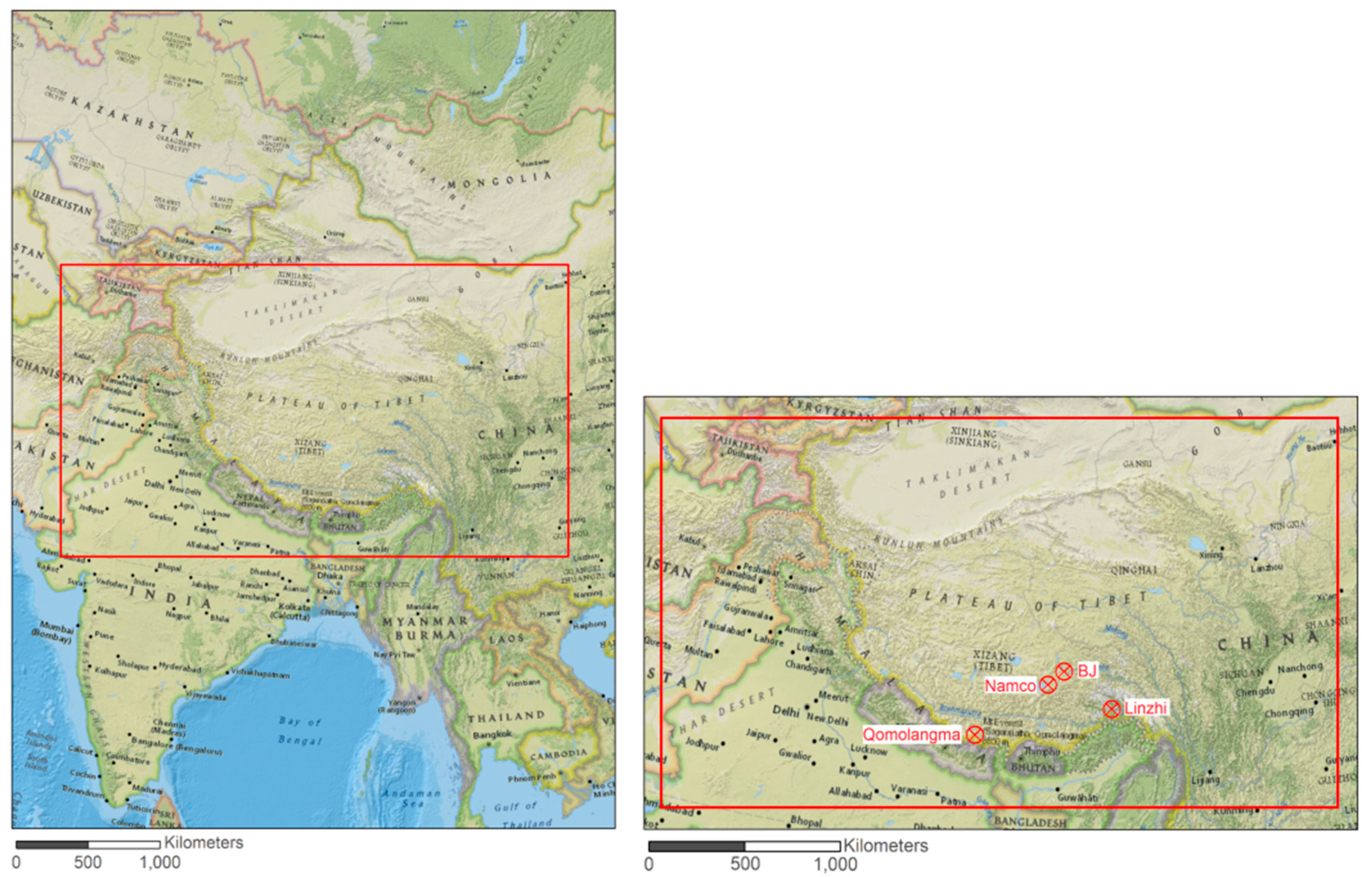
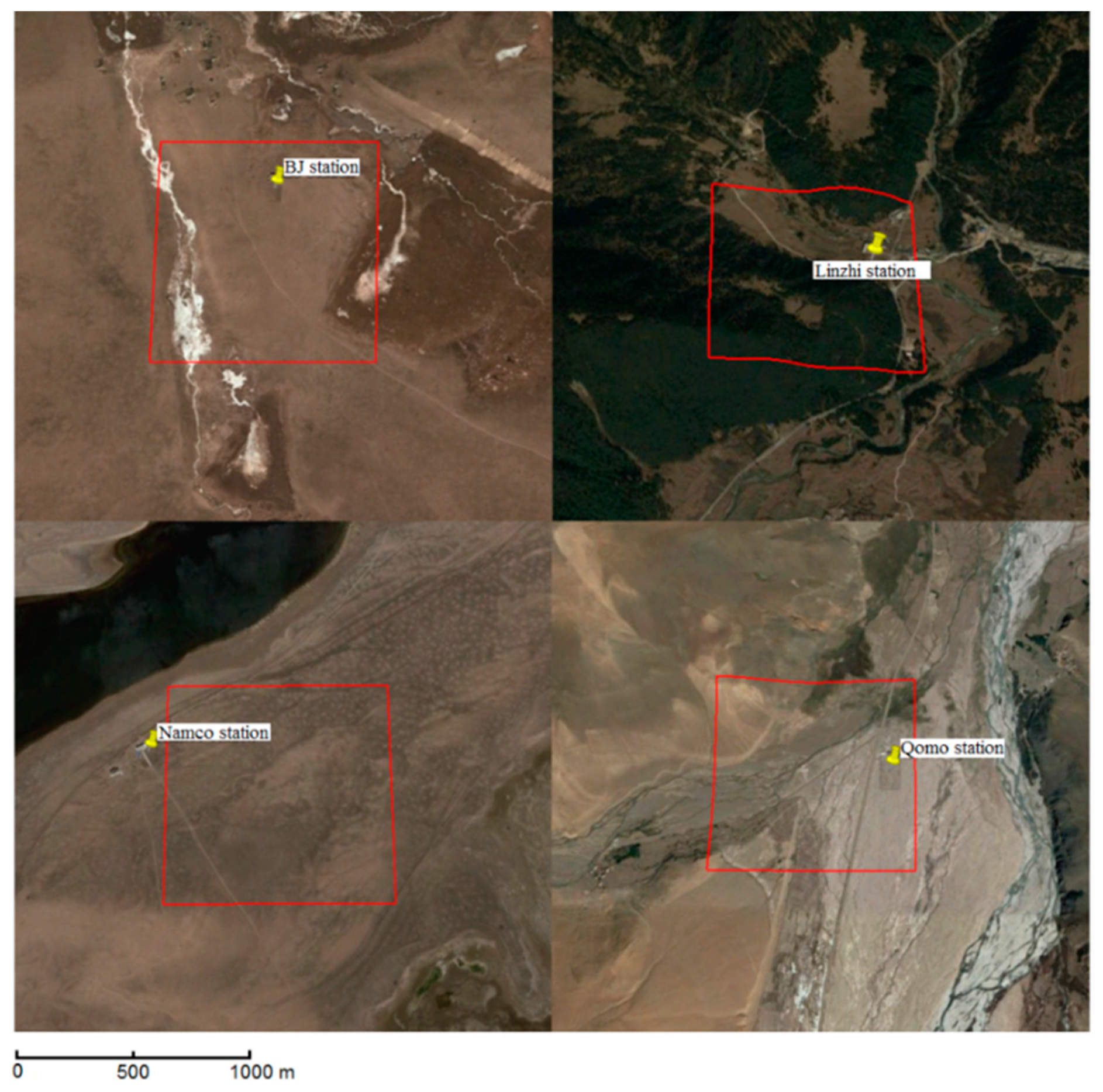
2.1. Study Area and Validation Data

The Tibetan Plateau, lying between the Himalayan range to the south and the Taklimakan desert to the north (Figure 1), is the largest and highest plateau area in the world spreading over 1.2 million km² and presenting an average elevation over 5000 meters. Ground measurements, coming from four radiative balance stations located on the Tibetan Plateau (Figure 1): BJ (now Nagqu), Linzhi, NamCo, and Qomolangma, are used to evaluate the modelled solar radiation budget estimates. The information concerning the stations’ sites and instruments is taken from Babel et al. [26]. The BJ site is set over relatively flat terrain in a large valley at 4502 m. The vegetation is very low, sometimes interspersed with bare soil, but quite homogeneous on the landscape scale. The nearest hill slopes are located at about 1 km away. The Linzhi station, lying at 3327 m, is located at the start of a small valley in an area covered by an alpine meadow with tall grasses and herbs during the summer period, while the meadows outside of the site are grazed and thus very short. The landscape is very heterogeneous with steep slopes, covered by mixed forest. The pastures outside the fence alternate with a small creek and bushes and single trees, respectively. The NamCo station, at 4730 m, is located on the southeast shore of the NamCo Lake, which is the second largest saline lake in the Tibetan Plateau. The station is surrounded by several mountain ranges, especially the Nyenchentanglha mountain range in the South. The measurement site itself is settled over a flat terrain, and the typical vegetation around the station is an alpine steppe. The Qomolangma Atmospheric and Environmental Observation and Research Station lies at 4276 m above sea level located at 30 km from the Mount Everest. The station is set in a valley enclosed by steep slopes at a distance of 750 m east and 500 m north-west and south-west of the tower with a height of about 600–800 m above ground level. A side valley comes in from the west. The site land cover is dominated by riverbed gravel, with very sparse vegetation, but also small patches of short alpine meadows.

2.2. Solar Radiation Budget from Remote Sensing

2.2.1. Instantaneous Solar Radiation

The solar radiation budget ($R_{ns}$) is defined as the difference between the incident ($R_{s\downarrow }$) and reflected ($R_{s\uparrow }$) solar radiative fluxes (W·m⁻²) at the surface at a certain time (Equation (1)):

$$R_{ns}=R_{s\downarrow }-R_{s\uparrow }$$

(1)

The estimation of the solar radiation budget requires an accurate quantification of the solar incident radiative flux reaching the Earth’s surface, commonly named irradiance and noted as $E$ hereafter, and the determination of the fraction of irradiance reflected by the surface, controlled by the surface albedo. Therefore, $R_{ns}$ can also be expressed as function of the surface albedo ($a$) and irradiance ($E$, W·m⁻²) as follows:

$$R_{ns}=\left(1-a\right)E$$

(2)

During the last few decades, many approaches were proposed to estimate surface irradiance using satellite measurements, at both regional and global scales, for a wide range of satellite data type, geostationary [27,28,29,30,31,32,33] or polar orbiting satellite [34,35,36]. However, most of the methods make use of geostationary satellite images [37], limiting the spatial resolution of the estimations. Raphael et al. [38], Pinker et al. [39], and Niemela et al. [7] provide a review for some of those methods which present different degree of complexity. Whatever the complexity of the model, the irradiance at the surface can be basically expressed as [7]:

$$E=S_0\times \cos {\theta }_s\times \tau$$

(3)

The solar zenith angle ${\theta }_s$ multiplied by the solar constant $S_0$ corrected for the sun-earth distance provides the top of the atmosphere (TOA) irradiance ($E_0$) for a given time of the day and a given day of the year. The last term of the equation, $\tau$, the atmospheric shortwave transmittance, allows to integrate the atmospheric effects and to estimate surface irradiance from extraterrestrial irradiance. Even if more complex estimations can be found, $S_0$ is mostly estimated for a given day of the year, considering astronomical parameter such as the sun-earth distance. The solar geometry depends on the day of the year as well as on the geographic coordinates of the location considered. For those computations, the main guidelines followed in this paper are based on Iqbal [40].

In this method, $\tau$ is the variable derived from satellite data. As described in several publications [1,41,42,43,44], $\tau$ is influenced by five radiation-damping processes: (1) Rayleigh scattering; (2) aerosol extinction; (3) ozone absorption; (4) water vapor absorption; and (5) permanent gas absorption, leading to the partitioning of the extraterrestrial irradiance into direct, diffuse, and backscattered radiations. The atmospheric transmittance estimated and used in this study takes into account each of those processes, which can be respectively translated in the following spectral radiative transmittance factors: ${\tau }_r$, ${\tau }_a$, ${\tau }_{oz}$, ${\tau }_w$, ${\tau }_g$. The latter are then used to compute the spectral transmittance function of the atmosphere, defined by two elements: (1) the beam transmittance ($T_B$) and (2) the diffuse transmittance ($T_D$). The spectral radiative transmittance factors used to compute the broadband transmittance functions, come from Yang et al. [8] based on the Leckner’s spectral model [45]. The performance of this model was tested and verified in several studies [46,47,48,49]. For all sky conditions, the influence of clouds is taken into account by adapting the broadband transmittance function according to the parameterization described in Stephens et al. [50], also applied and validated in Van Laake et al. [1]. Once the broadband transmittance factors are computed, the beam and the diffuse transmittances can be calculated and the surface irradiance is then computed as follows:

$$E=S_0\times \cos {\theta }_s\times T_B+S_0\times \cos {\theta }_s\times T_D$$

(4)

The solar irradiance retrieval methods from remote sensing data are often applied considering flat terrain. Some methods were adapted or new ones developed to take into account the effects of topography on satellite measured data [51,52,53]. Those topographic corrections have been successful in improving the quality of the retrieved surface variables [54,55]. A common procedure applied in many algorithms to take into account topography is to use the average terrain slope and azimuth in the computation of the local illumination angle. In order to integrate the impact of topography, ${\theta }_s$ is replaced by the solar incident angle (${\theta }_i$). ${\theta }_i$ is computed at the satellite overpass time and is accounting for the terrain slope and azimuth derived from the DEM [56]. Then Equation (4) becomes:

$$E=S_0\times \cos {\theta }_i\times T_B+S_0\times \cos {\theta }_i\times T_D$$

(5)

2.2.2. Daily Solar Radiation

While the surface properties can be relatively constant over a day, assuming that there are no important changes of the surface conditions, the surface irradiance is varying over the day because it strongly depends on the sun geometry and atmosphere conditions, especially the presence of clouds. The surface irradiance is an instantaneous value computed at satellite overpass time which needs to be extrapolated to get the daily mean solar irradiance. There are several ways to proceed according to the data availability. For the sake of simplicity, the estimated albedo value is assumed as valid for the entire day. So, in order to characterize the solar irradiance at the surface, the variation in the Sun geometry and the state of the sky should also be taken into account. Regarding the Sun-target geometry, the solar zenith angle can be easily computed for each desired local time. To describe the state of the sky, one of the commonly used indicators is the total cloud cover which represents the fraction of the sky covered by clouds, usually measured at regular time intervals and averaged to a daily value. Thus, regular measurements over the day are required for their accurate estimation. When no information is available, the daily solar irradiance can be approximated using a sinusoidal function proposed by Bisht et al. [9], estimating the diurnal cycle of net solar radiation. In this function, the daily average net solar radiation ($R_{ns\_d}$), in terms of the instantaneous all skies shortwave radiation ($R_{ns}$) can be obtained using the local satellite overpass time ($t_{sat}$) as well as local sunrise ($t_{sr}$) and sunset time ($t_{ss}$):

$$R_{ns\_d}=\frac{2\times R_{ns}}{\left[\pi \times \sin \left(\pi \left(\left(t_{sat}-t_{sr}\right)/\left(t_{ss}-t_{sr}\right)\right)\right)\right]}$$

(6)

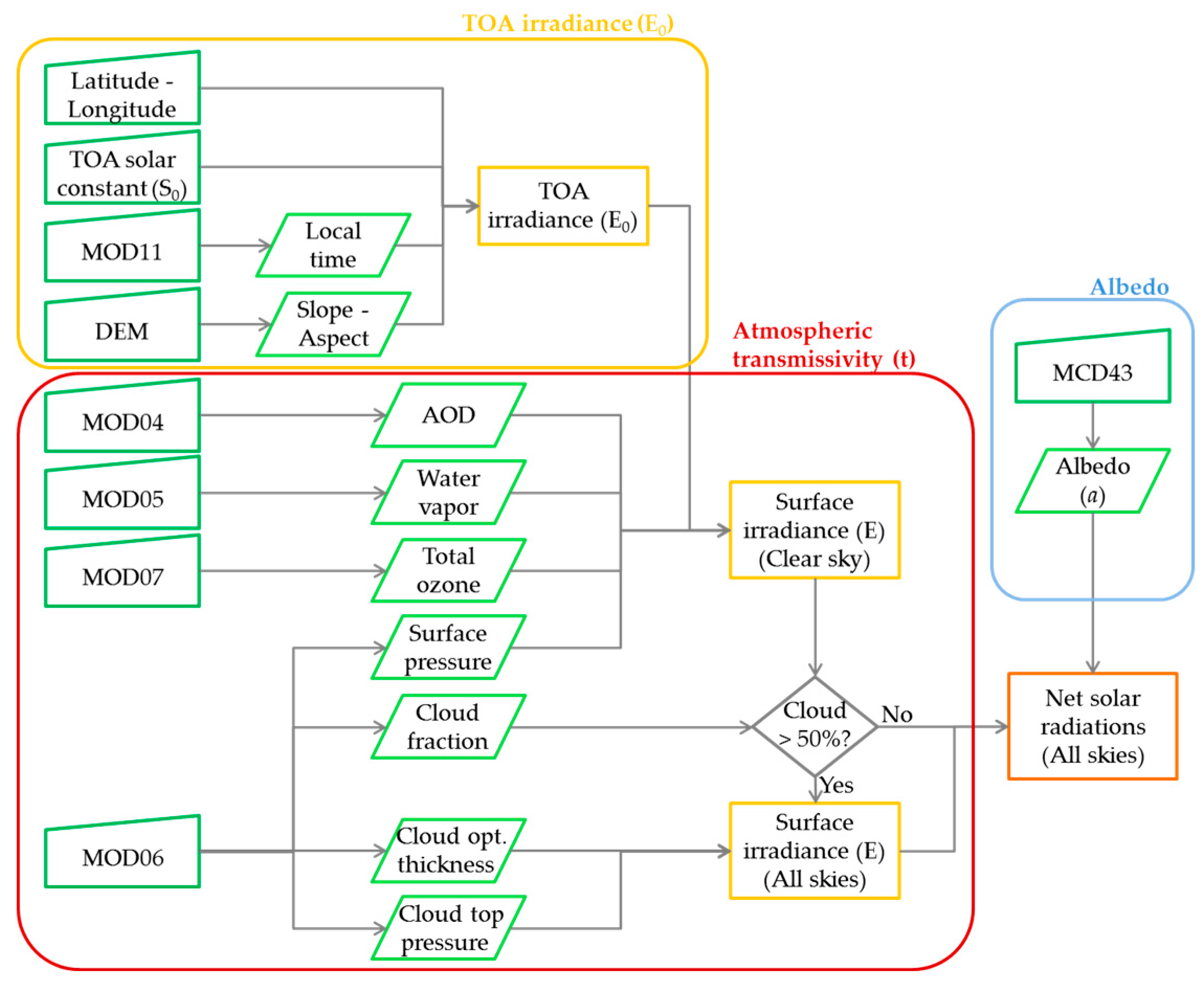
2.3. Solar Radiation Budget Using MODIS Data Products

MODIS data were selected because they are freely, widely and, for most of the products, have a kilometric resolution, and are available daily. However, when this study was conducted, MODIS albedo products were only available as eight-day products. Additionally, they are reliable and more than 10 years of archives are available allowing for the computation of historical averages and anomaly detection [3].

The methodology to estimate solar radiative fluxes over the Tibetan Plateau is implemented using Terra-MODIS atmospheric and land products level 2 and 3. All the atmospheric products are not related to the spectral wavelength and the albedo is a broadband product. Then, no narrow-to-broadband conversion is needed in this case as the produced solar radiative fluxes are directly broadband estimates. The surface pressure, atmospheric optical depth (AOD), the precipitable water, ozone thickness, and cloud properties are extracted from the level 2 atmospheric products. To compute the solar incident angle, the local satellite overpass time is necessary and is taken from MOD11A1 day view time. The black-sky and white-sky albedo are obtained from MCD43B3. Then, the blue-sky albedo is derived according to the method given in Román et al. [57]. All the required MODIS products are presented in

Table 1. MODIS data products level 2 used for the estimation of solar radiative fluxes.

Product Short Name	Product Group	Product Name	Spatial Resolution	Temporal Resolution	Data Layer Used
MOD04_L2	Atmosphere	Aerosol	10 km	Daily	Corrected optical depth land
MOD05_L2	Atmosphere	Water Vapor	5 km	Daily	Water vapor NIR retrieval
MOD06	Atmosphere	Cloud	1 or 5 km	Daily	Surface pressure Cloud top pressure Cloud fraction day Cloud optical thickness
MOD07	Atmosphere	Atmosphere profile	5 km	Daily	Total ozone
MOD11A1	Land	Land Surface Temperature & Emissivity	1 km	Daily	Day view time
MCD43B3	Land	Albedo	1 km	Eight-day	Black-sky albedo White-sky albedo

.

All the data products used during the solar radiative fluxes computation, except for the albedo product, are daily products and include missing data. Thus, a data filling plan was implemented in order to fill the gaps before using the data in the computation. The methodology applied is based on spatial and temporal gap filling. When there is less than 10% of missing data in a scene, local spatial average are used to fill the gaps. When there is more than 10% of missing data and if the corresponding eight-day or monthly MODIS level 3 products are available, the latter are used to fill the gaps. If missing pixels remain after this operation or if no eight-day or monthly MODIS products are available, the average value of the surrounding pixels is used. If there are still some pixels without value, the last option is to fill the pixel with the average value of the whole image (Figure 2). In parallel, a quality flag dataset is produced to provide information about the reliability of the estimates retrieved using those filled datasets.

Eight-day and monthly MODIS datasets are available for AOD, precipitable water, and ozone thickness. There is no such product available for the surface pressure data but this daily product is relatively complete, as shown later on (Section 3.4), then the use of the data filling procedure based on the local average is sufficient. The filling plan used the data presented in

Table 2. MODIS data products level 3 used for the daily products gap filling.

Product Short Name	Product Group	Product Name	Spatial Resolution	Temporal Resolution	Data Layer Used
MOD08_E3	Atmosphere	Eight-Day Joint product	1 degree	8-day	Corrected optical depth land Water vapor NIR retrieval Total ozone
MOD08_M3	Atmosphere	Monthly Global product	1 degree	1 month	Corrected optical depth land Water vapor NIR retrieval Total ozone

.

The characteristics of the topography are retrieved at 1 km resolution from the DEM provided by the Advanced Spaceborne Thermal Emission and Reflection Radiometer (ASTER), i.e., the Global Digital Elevation Model (GDEM) version 2. ASTER-GDEM2 is one of the most complete high-resolution digital topographic dataset in the world to date. The ASTER-GDEM2 covers land surfaces between 83°N and 83°S at a spatial resolution of 1 arc-second. Even if some geolocalization errors and elevation aberrations have been identified at the global scale, this dataset remains the best alternative in accessibility to high-quality elevation data for the selected study site [58].

2.3.1. Atmospheric Transmittance Clear Sky

The instantaneous irradiance at the surface ($E$) is estimated according to Equation (5). For clear sky conditions, the spectral radiative transmittance factors: ${\tau }_r$, ${\tau }_a$, ${\tau }_{oz}$, ${\tau }_w$, ${\tau }_g$, required to estimate the spectral transmittance function of the atmosphere, are calculated as follows [8]:

$$\overline{{\tau }_r}\approx \text{exp}(-0.008735ms\times {\left(0.547+0.014ms-0.00038m{s}^2+4.6\times {10}^{-6}m{s}^3\right)}^{-4.08})$$

(7)

$$\overline{{\tau }_a}\approx \text{exp}\left(\left(-m\right)\times b\times {\left(0.6777+0.1464\left(mb\right)-\left(0.00626\left({\left(mb\right)}^2\right)\right)\right)}^{-1.3}\right)$$

(8)

$$\overline{{\tau }_{oz}}\approx \text{exp}\left(-0.0365\left({\left(ml\right)}^{0.7136}\right)\right)$$

(9)

$$\overline{{\tau }_w}\approx \text{exp}\left(-0.05{\left(mw\right)}^{0.3097}-0.0138\times \ln \left(mw\right)-0.0581\right)$$

(10)

$$\overline{{\tau }_g}\approx \text{exp}\left(-0.0117m{s}^{0.3139}\right)$$

(11)

$l$ (cm⁻¹), $w$ (cm²·g⁻¹) and $b$ (km⁻¹) are the thickness of the ozone layer, the precipitable water and the Angstrom turbidity coefficient (0.406 × AOD), respectively. The air mass (m) and pressure corrected air mass (ms) are computed as:

$$m=1/\left(\sin {\alpha }_s+0.15{\left(57.296{\alpha }_s+3.885\right)}^{-1.253}\right)$$

(12)

$$ms=m\left(P/P_0\right)$$

(13)

With $P_0$ = 1.013 × 10⁵ (Pa), P representing the surface pressure, accounting for the surface elevation and ${\alpha }_s$ the solar elevation angle.

Then, the broadband transmittance functions: the beam transmittance ($T_B$) and the diffuse transmittance ($T_D$) are computed from the Equations (7)–(11), as follows:

$$T_B\approx \overline{ {\tau }_{oz}}\times \overline{{\tau }_w}\times \overline{{\tau }_g}\times \overline{{\tau }_r}\times \overline{{\tau }_a}$$

(14)

$$T_D\approx 0.5\overline{ {\tau }_{oz}}\times \overline{{\tau }_w}\times \overline{{\tau }_g}\times \left(1-\overline{{\tau }_a}\times \overline{{\tau }_r}\right)$$

(15)

2.3.2. Atmospheric Transmittance All Skies

When the cloud cover fraction provided by MODIS (MOD06) is higher than 50%, the influence of clouds is taken into account by adapting the equations according to the parameterization described in Stephens et al. [50]. To do so, the direct beam and diffuse irradiance are first computed for the atmosphere above the clouds. In that case, the pressure-corrected air mass is calculated to the level of cloud top pressure ($P_c$)—not surface pressure anymore and the atmospheric water vapor content is assumed to be contained entirely below the cloud top. Those assumptions lead to modify the equations to estimate ($\overline{{\tau }_r}$), ($\overline{{\tau }_g}$) and ($\overline{{\tau }_w}$) while the ones for ($\overline{{\tau }_a}$) and ($\overline{{\tau }_{oz}}$) remain (Equations (16)–(18)).

$$\overline{{\tau }_r}\approx \text{exp}(-0.008735mc{\left(0.547+0.014mc-0.00038m{c}^2+4.6\times {10}^{-6}m{c}^3\right)}^{-4.08})$$

(16)

$$\overline{{\tau }_w}\approx 1$$

(17)

$$\overline{{\tau }_g}\approx \text{exp}\left(-0.0117m{c}^{0.3139}\right)$$

(18)

With the pressure corrected air mass:

$$mc=m \left(P_c/P_0\right)$$

(19)

A broadband cloud transmittance factor (${\tau }_c$) is added to integrate the effect of the cloud on the shortwave radiation transmissivity. It uses the optical thickness of the clouds ($otc$) and a coefficient ($bet$) linearly interpolated from the values given in Stephens et al. [50] (Equation (20)). For the sake of simplicity when considering the dependency of cloud absorption to wavelength, Stephens et al. [50] provided values for two broad intervals of the solar spectrum. The first spreads from 0.3 to 0.75 μm, where the absorption of the solar radiation by the clouds is extremely small and the second which extends from 0.75 to 4 μm and integrates the absorption by the clouds.

$${\tau }_c=1-\left[\left(\left(bet\times otc\right)/\cos {\theta }_s\right)/\left(1+\left(bet\times otc\right)/\cos {\theta }_s\right)\right]$$

(20)

Finally ${\tau }_c$ is integrated to the direct beam transmittance factor by adapting Equation (14) as shown in Equation (21) and the surface solar irradiance is still estimated with Equation (5).

$$T_B=\overline{{\tau }_{oz}}\times \overline{{\tau }_w}\times \overline{{\tau }_g}\times \overline{{\tau }_r}\times \overline{{\tau }_a} \times {\tau }_c$$

(21)

All the cloud parameters required for the estimation of surface solar irradiance under cloudy condition, namely $P_c$, $otc$ and cloud fraction, are derived from the daily atmospheric products of MODIS (Table 1).

2.3.3. Solar Radiation Budget

Once the MODIS data products required for the estimation of the solar radiation budget are extracted, registered, and gap filled, the solar radiation budget can be computed in three main steps summarized in the workflow presented in Figure 3. First the TOA irradiance is calculated using the latitude and longitude values of each pixel, the solar constant corrected for the sun-earth distance, the satellite overpass time derived from MOD11A1 and integrating the slope and aspect of the terrain derived from the DEM. Second, the atmospheric transmissivity is computed for clear sky using the surface pressure, AOD, precipitable water, ozone thickness extracted from MOD06, MOD04, MOD05, and MOD05, respectively. Combined with the TOA irradiance, the surface irradiance is computed for clear sky. An atmospheric transmission factor for all sky conditions is also computed based on the cloud top pressure, the cloud optical thickness and the cloud fraction extracted from MOD06. Finally, the last step consists in deriving the blue sky albedo from MCD43B3 black and white-sky albedos and combining it with the all skies irradiance to estimate the solar radiation budget.

In order to reach the objective of daily monitoring, the instantaneous solar radiation budget is converted into daily average. As the method to retrieve the instantaneous solar radiative fluxes is only based on MODIS data, there are too few measurements over the day to characterize the evolution of the state of the sky or the sunshine duration, then the daily solar radiation is approximated using Equation (6).

3. Results

During the development of the method to estimate the solar radiation budget, some efforts have been done to represent the spatial and temporal heterogeneity of the Tibetan Plateau affecting the solar radiative fluxes over space and time. The computation of surface irradiance using an atmospheric transmission factor (Figure 4a,b) and considering terrain mean slope and azimuth to estimate the sun incident angle (Figure 4c,d), both at the kilometric resolution, highlights the importance of accounting for the spatial heterogeneity in that area.

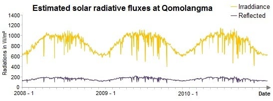
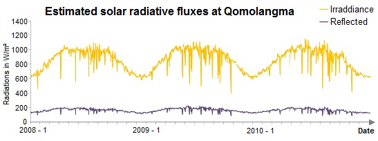
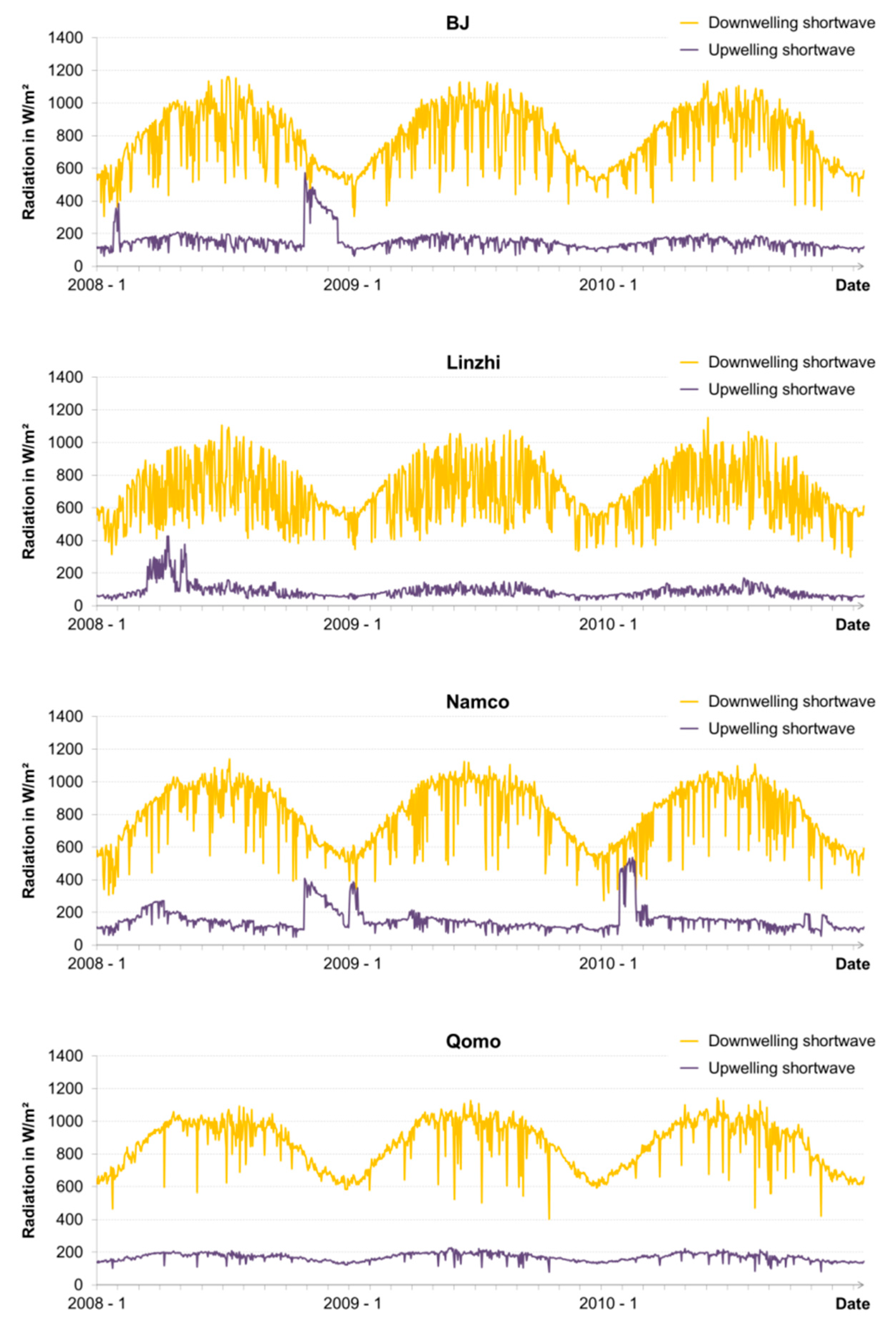
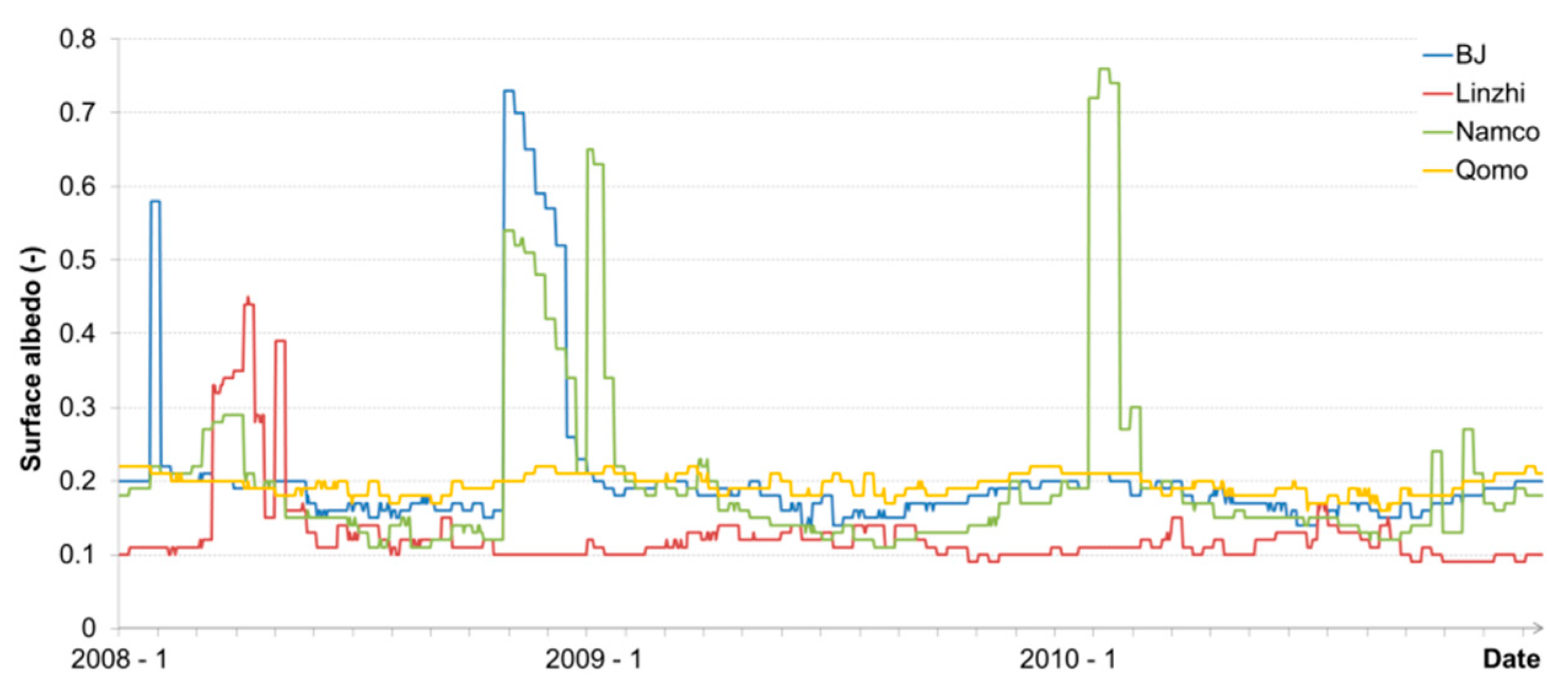
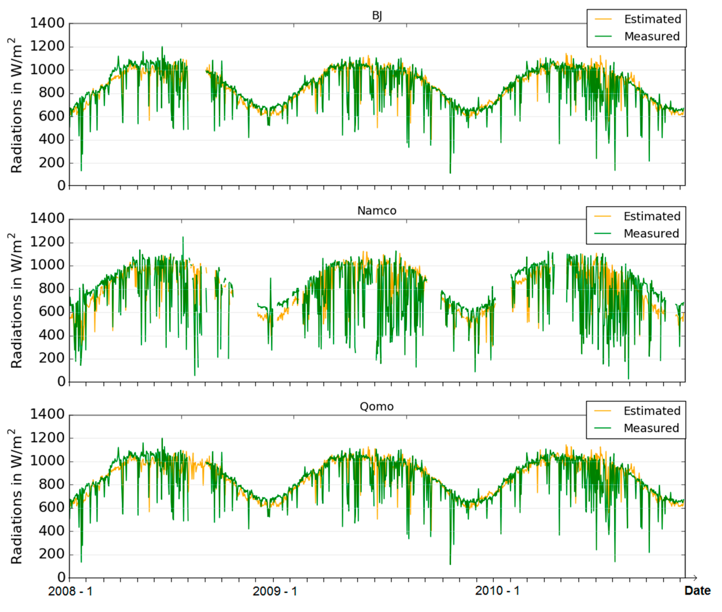
3.1. Solar Radiation Budget Three-Year Time Series

Based on the methodology presented in Section 2.3 and using a database containing the required gap filled MODIS products, a time series of instantaneous and daily at-surface solar radiative fluxes from 2008 to 2010 was produced at one kilometer resolution. Figure 5 shows the three-year time series of instantaneous solar irradiance and reflected fluxes estimated for the four pixels corresponding to the four ground stations, namely BJ, Linzhi, NamCo, and Qomolangma (noted as Qomo). The instantaneous values are estimated at satellite overpass time which is between 10.30 and 11 am local time depending on the day.

Figure 5 shows that the instantaneous solar incident and reflected radiative fluxes estimated at BJ, Linzhi and NamCo fluctuates more than the one obtained over Qomolangma. One of the reasons could be the lower yearly cloud fraction recorded over Qomolangma, according to the MODIS cloud products. For Qomolangma, the averaged cloud fraction over the three years is about 29%, while it is around 42%, 80%, and 46% for BJ, Linzhi, and NamCo, respectively. As the incident and reflected radiations are correlated, most of the fluctuations are similar. However, some sudden increases in reflected radiation are also observed for BJ, Linzhi, and NamCo stations. As the reflected fluxes (purple line in Figure 5) are derived using the MODIS albedo product, those increases are directly linked to increases of the MODIS albedo values. Figure 6 provides the time series of those MODIS albedo values (MOD43B3) for the same period and locations. From this figure, the same peaks are identified in the time lines. Those high values of surface albedo may be caused by the presence of snow on the ground. Surprisingly, no peak is observed for Qomolangma where snow events usually occur between mid-October and mid-May. This may be due to the fact that it rapidly melts after snowing and seldom lasts more than one day (Wang Zhongyan, personal communication, 31 March 2015). Thus, the MODIS albedo product used in this study, which is an eight-day product, seems to miss those snow events as at least eight individual days of snow were recorded at the station between mid-2008 to the end of 2010.

When visually checking the time series outputs, it appeared that, for some days and in area where the slope is very steep, some pixels present extreme values. One of the reasons is that the algorithms used in this method have been developed and tested on more homogeneous areas than the Tibetan Plateau and then the specificities of the Plateau go beyond their range of operation. However, those extreme values represent a small amount of pixels (less than 2% of the entire image) and, in the developed method, are filtered out and replaced by the average of the surrounding pixels values.

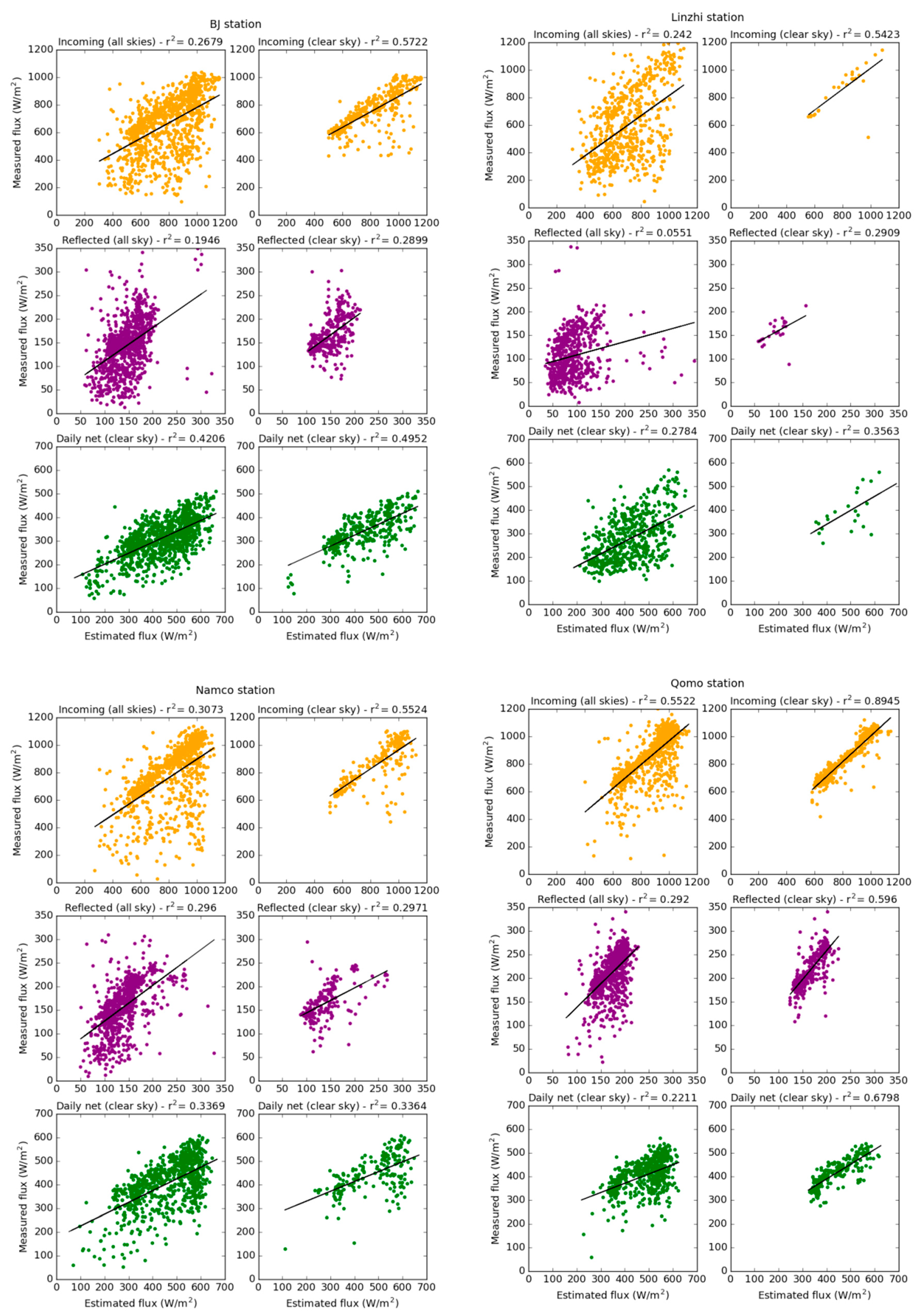
3.2. Validation Against Ground Measurements

The radiative fluxes estimates are validated using the ground measurements recorded at the four stations from 2008 to 2010, considering all skies and clear sky days separately. The distinction between clear sky and cloudy conditions is made on the basis of the cloud fraction provided by MODIS. Some incoherent values were observed in the ground measured reflected fluxes, then the data have been filtered which also masked out some possible snow events. The validation results are presented in the scatter plot in Figure 7.

According to Figure 7, better results are obtained when the solar radiative fluxes are estimated for clear sky, especially the instantaneous irradiance. The estimation of the latter performs also better than for the instantaneous reflected fluxes and the daily net radiations. Concerning the daily net radiations, the difference between all skies and clear sky conditions is less pronounced, except for Qomolangma station. This may be explained by the use of the sinusoidal function from [9] for the conversion of an instantaneous to a daily value, which does not account for the diurnal variation of cloud coverage and water vapor. After filtering out the cloudy days and the invalid data, only 14 clear sky days were available for validation at Linzhi station. For this reason, this station will not be further used for the validation. To deepen this validation, more statistics are provided in

Table 3. Solar radiative flux validation statistics for instantaneous incident fluxes, reflected fluxes, and daily net solar radiation. The bias (W·m⁻²), root-mean-square-error (RMSE, W·m⁻²) and r² are provided for all and clear skies conditions, at BJ, Qomo, and NamCo stations for the entire time series.

		BJ		NamCo		Qomo
		All Skies	Clear Sky	All Skies	Clear Sky	All Skies	Clear Sky
Instantaneous incoming	Bias	120.1	42.2	39.5	−12.9	13.0	−16.2
	RMSE	225.5	126.5	203.5	120.7	117.1	49.8
	r2	0.27	0.57	0.31	0.55	0.55	0.89
Instantaneous reflected	Bias	2.0	−17.2	−17.3	−24.9	−37.9	−50.6
	RMSE	48.7	36.8	49.0	43.4	53.6	56.0
	r2	0.19	0.29	0.30	0.30	0.29	0.60
Net daily	Bias	116.9	91.1	39	21.7	38.6	11.3
	RMSE	147.1	120.4	96.9	82.4	77	33.6
	r2	0.42	0.50	0.34	0.34	0.22	0.68

: the bias (Equation (22)), the root-mean-square-error (RMSE) (Equation (23)), and the r square from Figure 7.

$$\text{bias}=\frac{1}{n} {\displaystyle \sum }_{i=1}^{n}estimate{d}_i-measure{d}_i$$

(22)

$$\text{RMSE}=\sqrt{\frac{1}{n}{\displaystyle \sum }_{i=1}^n{\left(estimate{d}_i-measure{d}_i\right)}^2}$$

(23)

The statistics presented in Table 3 confirm that better results are obtained for clear sky. For all the stations, the instantaneous irradiance is globally overestimated for all skies while it is slightly underestimated for clear sky at NamCo and Qomolangma and overestimated at BJ. The comparison between estimated and measured instantaneous incident fluxes is also presented as a timeline in Figure 8 illustrating the underestimation for clear sky and the overestimation for all skies in NamCo and Qomolangma. On the contrary, the instantaneous reflected fluxes are generally underestimated and more important bias values are observed for clear sky. The RMSE computed for the instantaneous fluxes are relatively high, with less difference between all skies and clear sky for the reflected fluxes. However, it is important to recall that the RMSE penalizes variance as it gives errors with larger absolute values more weight than errors with smaller absolute values [59]. For clear sky incoming fluxes, most of the values are located close to the trend line (Figure 7) while few pixels show large difference between measured and estimated fluxes. Those large differences have a strong impact on the RMSE. Furthermore, part of the RMSE is explained by the bias which is, in some cases, important as compared to the RMSE. The observed bias may be caused by the fact that the instantaneous fluxes are compared to ground measurements interpolated from 30 min average values. As the cloud cover at a specific location can evolve rapidly, its impact on data integrated over 30 minutes can be important [60]. Moreover, at this time of the day, the solar radiative fluxes can increase rapidly in 30 min. Finally, the correlation between estimated and measured instantaneous and daily fluxes is mostly significant at the station of Qomolangma and only for clear sky conditions. The better results obtained at this station are probably due to the more stable weather (less fluctuations in Figure 5) in this area and the lower yearly cloud fraction as presented in Section 3.1. The bias and the RMSE obtained for the validation of the net daily radiations shows values that are coherent with the results obtained for the instantaneous fluxes. It seems that in this case, even if very simple, the sinusoidal function applied for the conversion into daily fluxes does not introduce much more distortion. Moreover, the low difference between all skies and clear sky in this case is explained by the fact that the definition of clear sky is based on the sky conditions at the satellite overpass time.

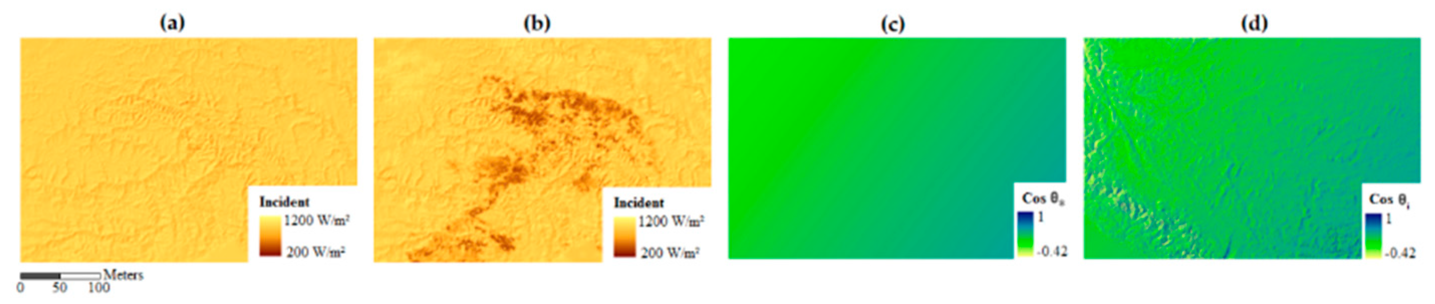
3.3. Evaluation of the Topographic Correction

Unlike most of the existing solar radiations products, this method integrated the impact of topography by correcting for the local illumination angles based on slope and aspect derived from the DEM. In order to evaluate the effectiveness of this topographic correction, incident fluxes, and daily net radiation estimated with and without correction are compared to ground measurements. For this analysis, only the Qomolangma station is considered as the other sites are located on very flat ground. Using the ground measurements provided for the whole year 2009 at this station, the fluxes estimated with and without topographic correction are evaluated and the corresponding bias, RMSE and r-square values are computed.

Table 4. Comparison of solar radiative fluxes estimated with and without topographic correction at Qomolangma station for the year 2009. The bias (W·m⁻²), the RMSE (W·m⁻²) and the r-square are provided for all skies and clear sky.

		With Topographic Correction		Without Topographic Correction
		All Skies	Clear Sky	All Skies	Clear Sky
Instantaneous incoming	Bias	15.9	−11.3	−5.0	−37.8
	RMSE	116.0	49	117.1	63.1
	r2	0.55	0.89	0.55	0.90
Net daily	Bias	48.3	23.1	43.7	17.3
	RMSE	80.3	43.6	77.6	40.7
	r2	0.35	0.73	0.34	0.72

provides an overview of those statistics.

From Table 4, it appears that, even if globally better results are obtained after the topographic correction, the differences are very low. This is mainly due to the fact that, even if this station is surrounded by mountains, it is still located on a flat area limiting the validation possibilities concerning the impact of the topographic correction used in this method. The applied correction considering only the impact of the slope and orientation of the terrain neglects the contribution of the surrounding terrain which would have a larger influence at Qomolangma station.

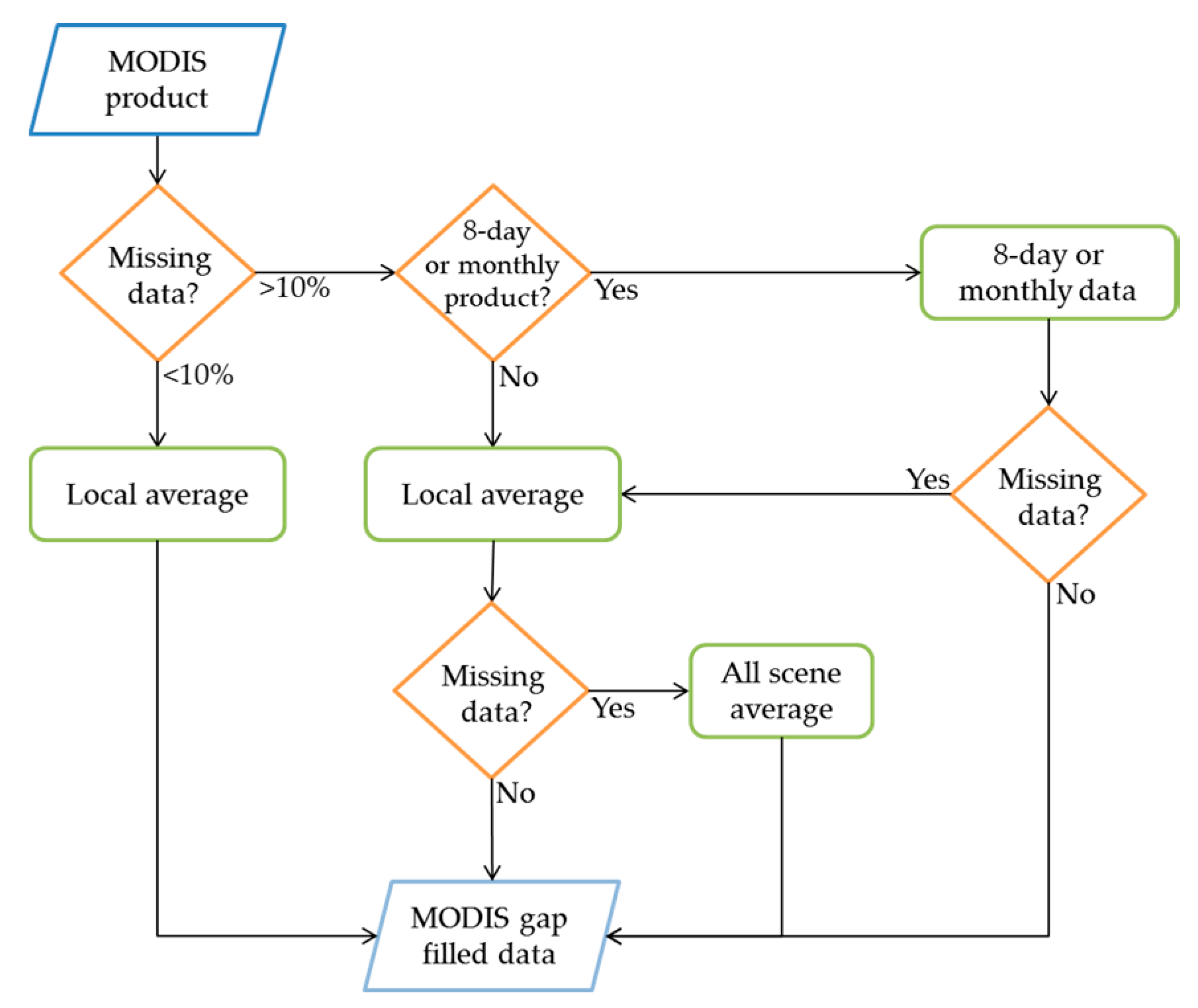
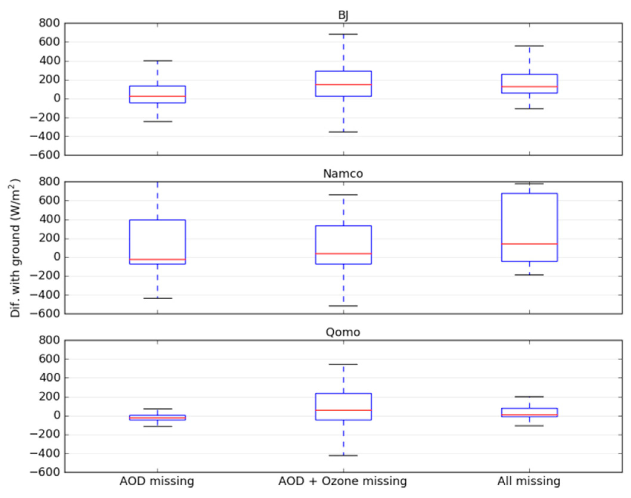
3.4. Evaluation of the Gap-Filling Procedure

Even if better results are obtained for clear sky conditions, the correlation between estimated and measured surface irradiance is quite low, except in Qomolangma station. The inaccuracy observed in the estimation of the incident radiation may be partially explained by the fact that some of the data used in the computation of the atmospheric transmissivity are scarcely available over the Plateau (

Table 5. Percentage of missing data for each of the atmospheric products used in the atmospheric transmissivity factor calculation.

	2008	2009	2010	Comments
Surface Pressure	2.2% (±0.6%)	2.4% (±3.2%)	2.2% (±0.6%)	Gaps between tiles
Precipitable Water	3.7% (±2.8%)	4.1% (±4.4%)	4% (±3.4%)	Gaps + missing data
Total Ozone	50% (±12.6%)	48.9% (±12.3%)	50.3% (±12%)	Missing data
AOD	84.5% (±4.9%)	83.9% (±4.6%)	84.7% (±4.6%)	Missing data

). Then, the missing data need to be replaced by less accurate estimates, like weekly or monthly average values (Figure 2), knowing that the quality of the output is directly linked to the quality of the input data. From Table 5, it appears clearly that the most problematic atmospheric variable is the AOD. However, due to the high altitude of the Tibetan Plateau, the atmosphere is thin and the AOD is very small over that area [61]. This can also be the reason for the important rate of missing data, i.e., the particular conditions of the Plateau may go beyond the limits of the AOD retrieval algorithm. Furthermore, except after a sand storm in the Gobi area, a limited variation in aerosol load was observed [62]. Then using monthly estimates should not be critical in this case.

In order to evaluate the impact of the missing data and the suitability of the gap-filling procedure the differences between estimated and measured instantaneous incoming fluxes observed for three different combinations of missing data are compared (Figure 9) based on the quality flag produced along with the estimations. The three selected combinations cover most of the observed missing data combinations: (1) only the AOD value was missing; (2) the AOD and the total ozone value are missing; and (3) all values are missing.

Figure 9 shows that good results are obtained when only the AOD is missing. As explained previously, the impact of AOD is very low on the Tibetan Plateau. The median error and the dispersion of the data increase when AOD and ozone are both missing, except for NamCo where the dispersion remains quite similar. Except in NamCo, the fact that more data than AOD and Ozone is missing does not affect the distribution of the observed errors. The different trend observed at the NamCo station may due to the presence of the lake very close by, influencing the retrieved atmospheric parameters. It is also important to keep in mind that, when data are missing, it is often due to important cloud cover or extreme conditions and, more than the influence of the gap-filling, this can also be the reason of the error increase. It is then difficult to evaluate the impact of the gap-filling procedure applied in this study. Nevertheless, it does not seem to cause an increase of the observed errors while allowing the production of a gap free dataset.

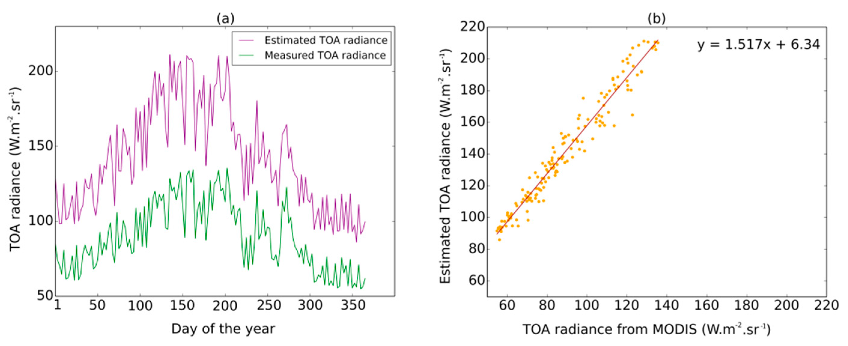
3.5. At-Sensor Validation

To deepen the validation of the solar radiation budget time series, a comparison with satellite data at the same spatial resolution is performed. This validation method allows to overcome the footprint issue faced when comparing satellite estimates to ground measurements over heterogeneous landscape, as illustrated later on (Section 4). The main objective is to verify if the retrieval of the atmospheric transmissivity for the estimation of surface irradiance is accurate. To do so, the surface irradiance is estimated following the proposed method. Next, the surface reflectance provided by MODIS products is used to compute the surface reflected radiance. The latter is then converted to TOA reflected radiance using atmospheric transmissivity values computed with the same approach but for the view zenith angle instead of the sun zenith angle. Finally, the estimated TOA reflected radiance is compared to the TOA reflected radiance measured by MODIS. The atmospheric transmissivity and the surface irradiance being estimated broadband, a prerequisite to this comparison is the conversion of the spectral reflectance and radiance data provided by MODIS to broadband estimates. The validation is performed over the study area subset (135 × 135 km, over strong topography in the South part of the Plateau) and over the whole year 2010, considering only clear sky days. The results of the comparison are presented in Figure 10.

This comparison highlights a constant shift between the estimated and the measured TOA reflected radiance. This is confirmed by the equation of the regression which shows a slope of 1.517 and an intercept very close to 0. There are two potential reasons for this shift. First, the assumptions made to convert the measured spectral radiance to broadband radiance could lead to an underestimation of the broadband radiance. As the land cover is relatively stable over the test area, this underestimation could generate a constant bias. Second, the atmospheric transmissivity computed by MODIS to retrieve the surface reflectance is lower than the one estimated with the approach proposed in this paper. In this study, the atmospheric transmissivity for clear days is around 0.9 which is confirmed by the data measured at the ground. It is also possible that those two potential errors add to each other. However, this comparison shows that the way the atmospheric transmissivity is modelled in the proposed method is providing suitable results for clear sky days and confirms that the problem mostly come from cloudy conditions. It also confirms the observation made in Section 3.4, that the gap-filling procedure does not influence the estimations under clear sky conditions. Thus, as the clear sky atmospheric transmissivity is correct, the surface irradiance retrieved for clear sky condition is also correct. Then, the low accuracy observed for the estimated reflected radiance under clear sky conditions (Figure 7), is probably caused by the MODIS albedo product. This is supported by the fact that the ground validation shows that the overall estimates of reflected radiance are worse than estimates of incident radiance with lower correlation between the ground measurements and the estimates, whatever the sky conditions.

3.6. Comparison with Evaluations of other Existing Radiative Fluxes Products over the Tibetan Plateau

In order to provide some first hints about the benchmark of the method as compared to some of the existing ones, a comparison with the error quantities provided in the literature for those products is discussed. However, only a direct inter-comparison of different methods at the same stations and for the same time period could provide an accurate benchmarking of the different methods. The comparison of our estimations with other existing products is based on the results provided in two papers: Gui et al. [63] and Yang et al. [21]. It is important to keep in mind that the incident and reflected fluxes validated in our paper are instantaneous values, not hourly or three-hourly means, which make the results more sensitive to dispersion, especially when evaluated against 30 minutes average observations provided by the ground station.

The CERES-FSW product is evaluated over the Tibetan Plateau in Gui et al. [63]. This paper shows positive biases for individual sites ranging from 8.0 W·m⁻² to 131.4 W·m⁻² and RMSEs ranging from 139.0 W·m⁻² to 236.7 W·m⁻² for the CERES incident solar fluxes. For the reflected fluxes, biases for individual sites range from −17.1 W·m⁻² to 35.3 W·m⁻² and RMSEs range from 61.6 W·m⁻² to 114.8 W·m⁻². The validation of the incident fluxes estimations provided by the method proposed in this paper shows biases ranging from −16.2 W·m⁻² to 120.1 W·m⁻² and RMSEs ranging from 49.8 W·m⁻² to 225.5 W·m⁻². The validation results of those two products are comparable for the incident fluxes. This is not the case for the reflected fluxes as, in this paper, the biases range from −50.6 W·m⁻² to 2 W·m⁻² and the RMSEs from 36.8 W·m⁻² to 56 W·m⁻². Overall, the results obtained with the proposed method over the Tibetan Plateau seem better than the ones from the CERES-FSW products, especially for clear sky where higher r² are observed.

Five solar incident fluxes products are validated over the Tibetan Plateau in Yang et al. [21]. The validation period covers, at most, 92 days while we used three years of estimation and is done using three-hour averages, which filter out faster deviations over shorter periods of time between ground observations and estimated data. Even then, the standard deviations of the difference between three hours mean observations and satellite products remain pretty high and range between 57.4 W·m⁻² and 112.4 W·m⁻². In our case, the validation for incident fluxes, performed with instantaneous estimates and 30 min average ground data, gave RMSEs ranging from 117.1 W·m⁻² to 225.5 W·m⁻² for all sky conditions and 49.8 W·m⁻² to 126.5 W·m⁻² for clear sky. The radiative fluxes estimations presented in this paper are less accurate under cloudy conditions, but similar accuracy to the one provided for the validation of the other products is reached under clear sky. Concerning the daily fluxes, the use of the sinusoidal function from Bisht et al. [9] to go from instantaneous to daily solar radiations is an approximation and leads to high RMSEs as compared to the one provided by other products.

4. Discussion

The validation showed better solar radiative flux retrieval for clear sky and especially for instantaneous irradiance. The quality and the availability of the MODIS data products used in the method have been quoted as a potential source of error. The temporal difference between the time used in the computation, which is the exact MODIS overpass time, and the 30 min average ground observations used for the validation was also mentioned, especially linked to the rapid evolution of the cloud cover over the Plateau. Considering this point, the distinction between clear sky and cloudy sky for the validation based on the MODIS cloud fraction information was also analyzed. A small test was run to identify the cloudy conditions based on the difference between the ground measurements and the top of atmosphere irradiance. The later showed that the days identified as cloudy according to this method were significantly different that the ones identified as cloudy based on the MODIS cloud fraction. This discrepancy could lead to the lower correlation observed at BJ and Namco for incident fluxes estimation under clear sky. Another explanation for the low correlation between the estimated and the measured fluxes is linked to the spatial footprint of the two compared datasets. Those errors add up to the error due to the inaccuracy of the computation. First, the use of ground measurements at higher temporal resolution would improve the validation. Second, it is necessary to assess the impact of the spatial footprint when validating a variable estimated from remote sensing with ground measurement. As shown in Figure 11, the stations are located within pixels comprising several land cover types. Then the measurements collected at the stations are not representative of the pixel heterogeneity. Several studies stressed that a direct comparison is very challenging because of this scale issue and the heterogeneity of the land surface at the satellite spatial resolution that reduces the spatial representativeness of ground point measurements [64,65,66]. For each of the validation sites, the footprint was estimated considering the high of the instruments (between 1 and 2 m) and the field of view of the instrument. Because of the low position of the sensors, the footprint is very small as compared to the kilometric pixel of the satellite and the spatial variation of the surface is low. In Figure 11, the site of NamCo appears to be outside of the satellite footprint (red box). This pixel was selected for the comparison with the NamCo site because the pixel actually covering this site also includes part of the lake. The presence of water in the pixel would generate distortions in the validation procedure. Furthermore, the land cover and the topography in the selected pixel are very similar to the one of the NamCo site.

The validation also pointed out that the estimation of the instantaneous reflected fluxes is less accurate than the estimation of the instantaneous irradiance and that the difference between all skies and clear sky is smaller. Two main reasons can be put forward. First, the accuracy of the MODIS albedo product is not satisfying on the Tibetan Plateau due to its strong topography. Indeed several studies showed that, for global surface albedo products, e.g., MODIS or AVHRR, the effect of topography is an important source of error if retrieval assumes a horizontal surface [67] and that those products have limited accuracy in areas as rugged as the Tibetan Plateau [68]. As the topographic correction integrated in the estimation of the irradiance, a topographic correction should also be introduced in the retrieval procedure of the albedo. Furthermore, the MODIS albedo product used in this study provides a value every eight days. This temporal resolution is too coarse for the daily monitoring of radiative fluxes over the Tibetan Plateau which often undergoes fast changes. This product is now available daily [69], which would help improve the estimation over snowy conditions. In addition, the use of the albedo from either the overpass time or the local noon-adjusted value should be carefully considered as it would sometimes contribute to significant errors in net radiation estimation as a result of diurnal albedo variation.

The main limitations of this method are currently the use of the sinusoidal function to extrapolate the daily solar radiations from one instantaneous value and the fact of neglecting the contribution of the surrounding terrain in the topographic correction. Concerning the estimation of daily values, solutions should be explored to integrate the diurnal variation of cloud coverage and water vapor. This could be performed using the MODIS data product from the AQUA platform to produce the instantaneous fluxes at another satellite overpass time and more accurately estimate the daily sunshine duration [70] or by extracting the cloud and water vapor information from other satellites such as geostationary satellites with a higher temporal resolution. About the topographic correction, even if integrating the impact of slope and orientation of the terrain is already an improvement as compared to other existing solar radiation products, the applied correction still remains very simple. The localization of the ground stations used in this study did not allow for an in-depth evaluation of the effectiveness of the applied topography correction. However, it is certain that integrating the impact the surrounding terrain besides the geometry changes is necessary in such a rugged area, as the adjacency effect is also an important factor. The impact of incident radiations reflected by the surrounding inclined surfaces has been highlighted in several studies [71,72,73,74]. As working at the square kilometer, the integration of sub-pixel topography may also improve the results as shown in [75].

5. Conclusions

The method proposed in this paper allows to model the solar radiation budget instantaneously and daily, at the square kilometer level over the entire Tibetan Plateau using MODIS data products. Even if the overall accuracy is equivalent to already existing products [21,63], this method provides solar radiation estimates at the square kilometer level on a daily basis whereas the other net radiation datasets covering that area provide the same estimates but at a coarser spatial or temporal resolution. Furthermore, it uses the local solar incident angle in the computation of irradiance while the terrain geometry is often neglected.

Using MODIS data products offers the advantage of freely available data, which are widely used and continuously improved. Those data are at a suitable spatial and temporal resolution for this study and 10 years of archived data for long-term analyses are available. This study highlighted the relevance of those products to model the atmospheric transmissivity for clear sky despite an important lack of AOD data over the Tibetan Plateau. The eight-day albedo product is not sufficient to properly estimate the reflected fluxes due to its low temporal resolution and the fact that its retrieval is probably affected by the topography of the underlying terrain. The use of the new daily MODIS albedo product may solve the temporal issue while some topographic correction should also be considered.

The method was tested and used to produce a three-year time series, from 2008 to 2010. As for other large scale solar radiation budget products, the validation remains an issue and shows some discrepancies with the ground data. To overcome this problem, a sensor comparison was also performed to evaluate the proposed method. It appears that a large part of the errors is due to the inaccuracy of the albedo product and to the integration of the clouds. Thus, the estimation of the solar radiation budget should be improved considering two main aspects. First, higher temporal resolution albedo products should be used and some effort should be put in the integration of the topographic effects when retrieving albedo from space. Second, further research should also be done to integrate better the effect of clouds on the instantaneous solar radiation estimates. It is also of interest to mention the lack of AOD data pointed out by the validation, even is the AOD is very low and quite constant over the Tibetan Plateau [61,62].

The main achievement of this study is to propose an operational method to produce solar radiation budget estimates at the square kilometer level on a daily basis, key input for further use in climatic models,. The main improvement brought by this method is then the higher resolution of the produced data and the integration of topography, even if the latter was still not sufficient to compensate for the very rough terrain of the Tibetan Plateau and should be improved to integrate the impact of surrounding terrain at pixel or at sub-pixel level. Some work should also be done to provide a better conversion from instantaneous to daily considering the cloud cover and water vapor variation over the day.

To conclude, this simple method is fully operational and based on freely available data, it offers the possibility to anyone to produce a reliable solar radiation budget dataset, keeping in mind the described limitations. The improvement of the existing data products, in parallel with the development of more efficient topographic correction and cloud integration, the method could be further improved.

References

1. Van Laake, P.E.; Sanchez-Azofeifa, G.A. Simplified atmospheric radiative transfer modelling for estimating incident PAR using MODIS atmosphere products. Remote Sens. Environ. 2004, 91, 98–113. [Google Scholar] [CrossRef]
2. Jia, L.; Menenti, M. Response of vegetation photosynthetic activity to net radiation and rainfall: A case study on the Tibetan Plateau by means of Fourier analysis of MODIS fAPAR time series. Adv. Earth Sci. 2006, 21, 1254–1259. [Google Scholar]
3. Jia, L.; Roupioz, L.; Hu, G.; Zhou, J. Anomalies Maps of Net Radiation, LST and FPAR, CEOP-AEGIS Deliverable Report De9.7; University of Strasbourg: Strasbourg, France, 2011. [Google Scholar]
4. Bisht, G.; Venturini, V.; Islam, S.; Jiang, L. Estimation of the net radiation using MODIS (Moderate Resolution Imaging Spectroradiometer) data for clear sky days. Remote Sens. Environ. 2005, 97, 52–67. [Google Scholar] [CrossRef]
5. Yang, K.; Koike, T.; Ye, B. Improving estimation of hourly, daily, and monthly solar radiation by importing global data sets. Agric. For. Meteorol. 2006, 137, 43–55. [Google Scholar] [CrossRef]
6. Dubayah, R. Estimating net solar radiation using landsat thematic mapper and digital elevation data. Water Resour. Res. 1992, 28, 2469–2484. [Google Scholar] [CrossRef]
7. Niemelä, S.; Räisänen, P.; Savijärvi, H. Comparison of surface radiative flux parameterizations Part II. Shortwave radiation. Atmos. Res. 2001, 58, 141–154. [Google Scholar] [CrossRef]
8. Yang, K.; Koike, T.; Huang, G.W.; Tamai, N. Development and validation of an advanced model estimating solar radiation from surface meteorological data. In Recent Developments in Solar Energy; Hough, T.P., Ed.; Nova Science Publishers: Hauppauge, NY, USA, 2007. [Google Scholar]
9. Bisht, G.; Bras, R.L. Estimation of net radiation from the MODIS data under all sky conditions: Southern Great Plains case study. Remote Sens. Environ. 2010, 114, 1522–1534. [Google Scholar] [CrossRef]
10. He, T.; Liang, S.; Wang, D.; Shi, Q.; Goulden, M.L. Estimation of high-resolution land surface net shortwave radiation from AVIRIS data: Algorithm development and preliminary results. Remote Sens. Environ. 2015, 167, 20–30. [Google Scholar] [CrossRef]
11. Inamdar, A.; Guillevic, P. Net surface shortwave radiation from GOES imagery—Product evaluation using ground-based measurements from SURFRAD. Remote Sens. 2015, 7, 10788–10814. [Google Scholar] [CrossRef]
12. Wang, D.D.; Liang, S.; He, T.; Shi, Q.Q. Estimation of daily surface shortwave net radiation from the combined MODIS data. IEEE Trans. Geosci. Remote Sens. 2015, 53, 5519–5529. [Google Scholar] [CrossRef]
13. Tang, W.J.; Qin, J.; Yank, K.; Liu, S.M.; Lu, N.; Niu, X.L. Retrieving high-resolution surface solar radiation with cloud parameters derived by combining MODIS and MTSAT data. Atmos. Chem. Phys. 2016, 16, 2543–2557. [Google Scholar] [CrossRef]
14. Zhang, X.Y.; Li, L.L. Estimating net surface shortwave radiation from Chinese geostationary meteorological satellite FengYun-2D (FY-2D) data under clear sky. Opt. Express 2016, 24, A476–A487. [Google Scholar] [CrossRef] [PubMed]
15. Zhang, X.; Liang, S.; Wild, M.; Jiang, B. Analysis of surface incident shortwave radiation from four satellite products. Remote Sens. Environ. 2015, 165, 186–202. [Google Scholar] [CrossRef]
16. Zhang, T.; Stackhouse, P.W.; Gupta, S.K.; Cox, S.J.; Mikovitz, C. The NASA GEWEX surface radiation budget project: Dataset validation and climatic signal identification. In Proceedings of the International Radiation Symposium (IRC/IAMAS), Berlin, Germany, 6–10 August 2013; pp. 636–639.
17. Wielicki, B.A.; Barkstrom, B.R.; Baum, B.A.; Charlock, T.P.; Green, R.N.; Kratz, D.P. Clouds and the earth’s radiant energy system (CERES): Algorithm overview. IEEE Trans. Geosci. Remote Sens. 1998, 36, 1127–1141. [Google Scholar] [CrossRef]
18. Zhang, Y. Calculation of radiative fluxes from the surface to top of atmosphere based on ISCCP and other global data sets: Refinements of the radiative transfer model and the input data. J. Geophys. Res. 2004, 109, D9. [Google Scholar] [CrossRef]
19. Liang, S.; Zhao, X.; Liu, S.; Yuan, W. A long-term global land surface satellite (GLASS) data-set for environmental studies. Int. J. Digit. Earth. 2013, 6, 5–33. [Google Scholar] [CrossRef]
20. Ryu, Y.; Kang, S.; Moon, S.-K.; Kim, J. Evaluation of land surface radiation balance derived from moderate resolution imaging spectroradiometer (MODIS) over complex terrain and heterogeneous landscape on clear sky days. Agric. For. Meteorol. 2008, 148, 1538–1552. [Google Scholar] [CrossRef]
21. Yang, K.; Pinker, R.T.; Ma, Y.; Koike, T.; Wonsick, M.M.; Cox, S.J. Evaluation of satellite estimates of downward shortwave radiation over the Tibetan Plateau. J. Geophys. Res. 2008, 113, D17. [Google Scholar] [CrossRef]
22. Duguay, C.R. An approach to the estimation of surface net radiation in mountain areas using remote sensing and digital terrain data. Theor. Appl. Climatol. 1995, 52, 55–68. [Google Scholar] [CrossRef]
23. Ma, Y.; Su, Z.; Li, Z.; Koike, T.; Menenti, M. Determination of regional net radiation and soil heat flux over a heterogeneous landscape of the Tibetan Plateau. Hydrol. Process. 2002, 16, 2963–2971. [Google Scholar] [CrossRef]
24. Long, D.; Gao, Y.; Singh, V.P. Estimation of daily average net radiation from MODIS data and DEM over the Baiyangdian watershed in North China for clear sky days. J. Hydrol. 2010, 388, 217–233. [Google Scholar] [CrossRef]
25. Amatya, P.M.; Ma, Y.; Han, C.; Wang, B.; Devkota, L.P. Estimation of net radiation flux distribution on the southern slopes of the central Himalayas using MODIS data. Atmos. Res. 2015, 154, 146–154. [Google Scholar] [CrossRef]
26. Babel, W.; Eigenmann, R.; Ma, Y.; Foken, T. Analysis of Turbulent Fluxes and Their Representativeness for the Interaction between the Atmospheric Boundary Layer and the Underlying Surface on Tibetan Plateau; CEOP-AEGIS Deliverable Report De1.2; University of Strasbourg: Strasbourg, France, 2011. [Google Scholar]
27. Gautier, C.; Diak, G.; Masse, S. A simple physical model to estimate incident solar radiation at the surface from GOES satellite data. J. Appl. Meteorol. 1980, 19, 1005–1012. [Google Scholar] [CrossRef]
28. Masuda, K.; Leighton, H.G.; Zhanqing, L. A new parameterization for the determination of solar flux absorbed at the surface from satellite measurements. J. Clim. 1995, 8, 1615–1629. [Google Scholar] [CrossRef]
29. Perez, R.; Ineichen, P.; Moore, K.; Kmiecik, M.; Chain, C.; George, R. A new operational model for satellite-derived irradiances: Description and validation. Sol. Energy. 2002, 73, 307–317. [Google Scholar] [CrossRef]
30. Hammer, A.; Heinemann, D.; Hoyer, C.; Kuhlemann, R.; Lorenz, E.; Müller, R. Solar energy assessment using remote sensing technologies. Remote Sens. Environ. 2003, 86, 423–432. [Google Scholar] [CrossRef]
31. Deneke, H.M.; Feijt, A.J.; Roebeling, R.A. Estimating surface solar irradiance from METEOSAT SEVIRI-derived cloud properties. Remote Sens. Environ. 2008, 112, 3131–3141. [Google Scholar] [CrossRef]
32. Blanc, P.; Gschwind, B.; Lefèvre, M.; Wald, L. The HelioClim project: Surface solar irradiance data for climate applications. Remote Sens. 2011, 3, 343–361. [Google Scholar] [CrossRef] [Green Version]
33. Geraldi, E.; Romano, F.; Ricciardelli, E. An advanced model for the estimation of the surface solar irradiance under all atmospheric conditions using MSG/SEVIRI data. IEEE Trans. Geosci. Remote Sens. 2012, 50, 2934–2953. [Google Scholar] [CrossRef]
34. Tang, B.; Li, Z.L.; Zhang, R. A direct method for estimating net surface shortwave radiation from MODIS data. Remote Sens. Environ. 2006, 103, 115–126. [Google Scholar] [CrossRef]
35. Wang, H.; Pinker, R.T. Shortwave radiative fluxes from MODIS: Model development and implementation. J. Geophys. Res. Atmos. 2009, 114, D20. [Google Scholar] [CrossRef]
36. Perez, R.; Cebecauer, T.; Šúri, M. Semi-empirical satellite models. In Solar Energy Forecasting and Resource Assessment; Academic Press: Oxford, UK, 2013; pp. 21–48. [Google Scholar]
37. Polo, J.; Zarzalejo, L.F.; Ramírez, L. Solar radiation derived from satellite images. In Modeling Solar Radiation at the Earth’s Surface; Springer: Berlin, Germany, 2008; pp. 449–461. [Google Scholar]
38. Raphael, C.; Hay, J.E. An assessment of models which use satellite data to estimate solar irradiance at the Earth’s surface. J. Clim. Appl. Meteorol. 1984, 23, 832–844. [Google Scholar] [CrossRef]
39. Pinker, R.T.; Frouin, R.; Li, Z. A review of satellite methods to derive surface shortwave irradiance. Remote Sens. Environ. 1995, 51, 108–124. [Google Scholar] [CrossRef]
40. Iqbal, M. An Introduction to Solar Radiation; Academic Press: Oxford, UK, 1983. [Google Scholar]
41. Carroll, J.J. Global transmissivity and diffuse fraction of solar radiation for clear and cloudy skies as measured and as predicted by bulk transmissivity models. Sol. Energy 1985, 35, 105–118. [Google Scholar] [CrossRef]
42. Muneer, T.; Gul, M.S. Evaluation of sunshine and cloud cover based models for generating solar radiation data. Energy Convers. Manag. 2000, 41, 461–482. [Google Scholar] [CrossRef]
43. Yang, K.; Huang, G.W.; Tamai, N. A hybrid model for estimating global solar radiation. Sol. Energy 2001, 70, 13–22. [Google Scholar] [CrossRef]
44. Chen, R.; Kang, E.; Ji, X.; Yang, J.; Wang, J. An hourly solar radiation model under actual weather and terrain conditions: A case study in Heihe river basin. Energy 2007, 32, 1148–1157. [Google Scholar] [CrossRef]
45. Leckner, B. The spectral distribution of solar radiation at the earth’s surface—Elements of a model. Sol. Energy 1978, 20, 143–150. [Google Scholar] [CrossRef]
46. Gueymard, C.A. Direct solar transmittance and irradiance predictions with broadband models. Part I: Detailed theoretical performance assessment. Sol. Energy 2003, 74, 355–379. [Google Scholar] [CrossRef]
47. Gueymard, C.A. Direct solar transmittance and irradiance predictions with broadband models. Part II: Validation with high-quality measurements. Sol. Energy 2003, 74, 381–395. [Google Scholar] [CrossRef]
48. Paulescu, M.; Schlett, Z. A simplified but accurate spectral solar irradiance model. Theor. Appl. Climatol. 2003, 75, 203–212. [Google Scholar] [CrossRef]
49. Madkour, M.A.; El-Metwally, M.; Hamed, A.B. Comparative study on different models for estimation of direct normal irradiance (DNI) over Egypt atmosphere. Renew. Energy 2006, 31, 361–382. [Google Scholar] [CrossRef]
50. Stephens, G.L.; Ackerman, S.; Smith, E.A. A shortwave parameterization revised to improve cloud absorption. J. Atmos. Sci. 1984, 41, 687–690. [Google Scholar] [CrossRef]
51. Proy, C.; Tanré, D.; Deschamps, P.Y. Evaluation of topographic effects in remotely sensed data. Remote Sens. Environ. 1989, 30, 21–32. [Google Scholar] [CrossRef]
52. Meyer, P.; Itten, K.I.; Kellenberger, T.; Sandmeier, S.; Sandmeier, R. Radiometric corrections of topographically induced effects on Landsat TM data in an alpine environment. ISPRS J. Photogramm. Remote Sens. 1993, 48, 17–28. [Google Scholar] [CrossRef]
53. Richter, R. Correction of atmospheric and topographic effects for high-spatial-resolution satellite imagery. Proc. SPIE 1997, 18, 216–224. [Google Scholar] [CrossRef]
54. Riano, D.; Chuvieco, E.; Salas, J.; Aguado, I. Assessment of different topographic corrections in Landsat-TM data for mapping vegetation types. IEEE Trans. Geosci. Remote Sens. 2003, 41, 1056–1061. [Google Scholar] [CrossRef]
55. Richter, R.; Kellenberger, T.; Kaufmann, H. Comparison of topographic correction methods. Remote Sens. 2009, 1, 184–196. [Google Scholar] [CrossRef] [Green Version]
56. Allen, R.G.; Trezza, R.; Tasumi, M. Analytical integrated functions for daily solar radiation on slopes. Agric. For. Meteorol. 2006, 139, 55–73. [Google Scholar] [CrossRef]
57. Román, M.O.; Schaaf, C.B.; Lewis, P.; Gao, F.; Anderson, G.P.; Privette, J.L. Assessing the coupling between surface albedo derived from MODIS and the fraction of diffuse skylight over spatially-characterized landscapes. Remote Sens. Environ. 2010, 114, 738–760. [Google Scholar] [CrossRef]
58. Li, P.; Shi, C.; Li, Z.; Muller, J.-P.; Drummond, J.; Li, X. Evaluation of ASTER GDEM using GPS benchmarks and SRTM in China. Int. J. Remote Sens. 2013, 34, 1744–1771. [Google Scholar] [CrossRef]
59. Chai, T.; Draxler, R.R. Root mean square error (RMSE) or mean absolute error (MAE)? Arguments against avoiding RMSE in the literature. Geosci. Model. Dev. 2014, 7, 1247–1250. [Google Scholar] [CrossRef]
60. Roupioz, L.; Colin, J.; Jia, L.; Nerry, F.; Menenti, M. Quantifying the impact of cloud cover on ground radiation flux measurements using hemispherical images. Int. J. Remote Sens. 2015, 36, 5087–5104. [Google Scholar] [CrossRef]
61. Xin, J.; Wang, Y.; Li, Z.; Wang, P.; Hao, W.M.; Nordgren, B.L. Aerosol optical depth (AOD) and Ångström exponent of aerosols observed by the Chinese Sun Hazemeter Network from August 2004 to September 2005. J. Geophys. Res. Atmos. 2007, 112, D5. [Google Scholar] [CrossRef]
62. Xia, X.; Wang, P.; Wang, Y.; Li, Z.; Xin, J.; Liu, J. Aerosol optical depth over the Tibetan Plateau and its relation to aerosols over the Taklimakan Desert. Geophys. Res. Lett. 2008, 35. [Google Scholar] [CrossRef]
63. Gui, S.; Liang, S.; Li, L. Validation of surface radiation data provided by the CERES over the Tibetan Plateau. In Proceedings of the 2009 17th International Conference on Geoinformatics, Fairfax, VA, USA, 12–14 August 2009.
64. Liu, S.; Liu, Q.; Liu, Q.; Wen, J.; Li, X. The angular and spectral kernel model for BRDF and albedo retrieval. IEEE J. Sel. Top. Appl. Earth Obs. Remote Sens. 2010, 3, 241–256. [Google Scholar] [CrossRef]
65. Liang, S.; Wang, K.; Zhang, X.; Wild, M. Review on estimation of land surface radiation and energy budgets from ground measurement, remote sensing and model simulations. IEEE J. Sel. Top. Appl. Earth Obs. Remote Sens. 2010, 3, 225–240. [Google Scholar] [CrossRef]
66. Cescatti, A.; Marcolla, B.; Santhana Vannan, S.K.; Pan, J.Y.; Román, M.O.; Yang, X. Intercomparison of MODIS albedo retrievals and in situ measurements across the global FLUXNET network. Remote Sens. Environ. 2012, 121, 323–334. [Google Scholar] [CrossRef]
67. Riihelä, A.; Manninen, T.; Andersson, K. Algorithm theoretical basis document—surface broadband albedo AVHRR/SEVIRI, EUMETSAT satellite application facility on climate monitoring. In EUMETSAT Satellite Application Facility on Climate Monitoring; EUMETSAT: Darmstadt, Germany, 2011. [Google Scholar]
68. Wen, J.; Zhao, X.; Liu, Q.; Tang, Y.; Dou, B. An improved land-surface albedo algorithm with DEM in rugged terrain. IEEE Geosci. Remote Sens. Lett. 2014, 11, 883–887. [Google Scholar]
69. Schaaf, C.B.; Wang, Z. MCD43A3 MODIS/Terra + Aqua BRDF/Albedo Daily L3 Global 500 m V006. Available online: http://0-doi-org.brum.beds.ac.uk/10.5067/MODIS/MCD43A3.006 (accessed on 11 June 2016).
70. Kandirmaz, H.M.; Kaba, K. Estimation of daily sunshine duration from terra and aqua MODIS data. Adv. Meteorol. 2014, 2014, 613267-9. [Google Scholar] [CrossRef]
71. Kawata, Y.; Ueno, S. Analytical and numerical simulation of satellite image from space. Comput. Math. Appl. 1999, 37, 123–131. [Google Scholar] [CrossRef]
72. Iikura, Y. Precise evaluation of topographic effects in satellite imagery for illumination correction. In Proceedings of the IGARSS 2008–2008 IEEE International Geoscience and Remote Sensing Symposium, Boston, MA, USA, 7–11 July 2008.
73. Sirguey, P. Simple correction of multiple reflection effects in rugged terrain. Int. J. Remote Sens. 2009, 30, 1075–1081. [Google Scholar] [CrossRef]
74. Sugawara, M.; Tanba, S.; Iikura, Y. Physically based evaluation of reflected terrain irradiance in satellite imagery for llumination correction. In Proceedings of the 10th WSEAS International Conference on Applied Computer Science, Iwate, Japan, 4–10 October 2010.
75. Roupioz, L.; Nerry, F.; Jia, L.; Menenti, M. Improved surface reflectance from remote sensing data with sub-pixel topographic information. Remote Sens. 2014, 6, 10356–10374. [Google Scholar] [CrossRef]
Figure 1. The Tibetan Plateau and surroundings, with the study area extent delimitation (red line), and location of the ground stations (circled red crosses) within the study area.
Remotesensing 08 00504 g001
Figure 2. MODIS daily products gap filling procedure.
Remotesensing 08 00504 g002
Figure 3. Computation of the instantaneous solar radiation budget for all skies using MODIS products and a DEM.
Remotesensing 08 00504 g003
Figure 4. Surface irradiance computed using: (a) a constant atmospheric transmission factor or (b) the proposed methodology and the solar geometry expressed as: (c) the solar zenith angle or (d) the sun incident angle.
Remotesensing 08 00504 g004
Figure 5. Time series of instantaneous solar incident (yellow) and reflected (purple) radiations for the pixels in which the ground stations used for the validation are located: BJ, Linzhi, NamCo, and Qomolangma (Qomo).
Remotesensing 08 00504 g005
Figure 6. Time series of surface albedo derived from MODIS (MOD43B3) over the four ground stations used for the validation: BJ (blue), Linzhi (red), NamCo (green), and Qomolangma (yellow).
Remotesensing 08 00504 g006
Figure 7. Solar radiative fluxes validation for instantaneous incident (orange) and reflected (purple) fluxes as well as daily net solar radiation (green). The validation is provided for all skies (left) or clear sky (right) conditions, at BJ, Qomo, Linzhi, and NamCo stations for the entire time series.
Remotesensing 08 00504 g007
Figure 8. Time series of estimated (yellow) and measured (green) instantaneous solar incident radiations for each of the pixel used for the comparison with the ground stations of BJ, NamCo, and Qomolangma (Qomo).
Remotesensing 08 00504 g008
Figure 9. Comparison of the differences in W·m−2 between estimated and measured instantaneous incoming fluxes at BJ, NamCo, and Qomolangma (Qomo) according to the input missing during the computation.
Remotesensing 08 00504 g009
Figure 10. Comparison between TOA reflected radiance estimated using MODIS surface reflectance and TOA reflected radiance measured by MODIS sensor: (a) mean TOA reflected radiance estimated (purple) and measured (green) for the entire study area; (b) the regression between the both mean TOA reflected radiance.
Remotesensing 08 00504 g010
Figure 11. The four ground stations location on the Tibetan Plateau (yellow pin) and the footprint of the pixel used for the validation (red lines). BJ (31°22’N, 91°53’E), Linzhi (29°45’N, 94°44’E), NamCo (30°46’N, 90°59’E), Qomo (28°21’N, 86°56’E).
Remotesensing 08 00504 g011