Article

Remote Sensing of Grass Response to Drought Stress Using Spectroscopic Techniques and Canopy Reflectance Model Inversion

Faculty of Geo-Information Science and Earth Observation (ITC), University of Twente, P.O. Box 217, 7500 AE Enschede, The Netherlands
*
Author to whom correspondence should be addressed.
Submission received: 14 April 2016 / Revised: 23 June 2016 / Accepted: 29 June 2016 / Published: 1 July 2016

Abstract

:
The aim of this study was to follow the response to drought stress in a Poa pratensis canopy exposed to various levels of soil moisture deficit. We tracked the changes in the canopy reflectance (450–2450 nm) and retrieved vegetation properties (Leaf Area Index (LAI), leaf chlorophyll content (Cab), leaf water content (Cw), leaf dry matter content (Cdm) and senescent material (Cs)) during a drought episode. Spectroscopic techniques and radiative transfer model (RTM) inversion were employed to monitor the gradual manifestation of drought effects in a laboratory setting. Plots of 21 cm × 14.5 cm surface area with Poa pratensis plants that formed a closed canopy were divided into a well-watered control group and a group subjected to water stress for 36 days. In a regular weekly schedule, canopy reflectance and destructive measurements of LAI and Cab were taken. Spectral analysis indicated the first sign of stress after 4–5 days from the start of the experiment near the water absorption bands (at 1930 nm, 1440 nm) and in the red (at 675 nm). Spectroscopic techniques revealed plant stress up to 6 days earlier than visual inspection. Of the water stress-related vegetation indices, the response of Normalized Difference Water Index (NDWI_1241) and Normalized Photochemical Reflectance Index (PRI_norm) were significantly stronger in the stressed group than the control. To observe the effects of stress on grass properties during the drought episode, we used the RTMo (RTM of solar and sky radiation) model inversion by means of an iterative optimization approach. The performance of the model inversion was assessed by calculating R2 and the Normalized Root Mean Square Error (RMSE) between retrieved and measured LAI (R2 = 0.87, NRMSE = 0.18) and Cab (R2 = 0.74, NRMSE = 0.15). All parameters retrieved by model inversion co-varied with soil moisture deficit. However, the first strong sign of water stress on the retrieved grass properties was detected as a change of Cw followed by Cab and Cdm in the earlier stages. The results from this study indicate that the spectroscopic techniques and RTMo model inversion have a promising potential of detecting stress on the spectral reflectance and grass properties before they become visibly apparent.

Graphical Abstract

1. Introduction

Plants are subjected to various harsh environmental conditions (i.e., abiotic stresses) in their ecosystems, which affect vegetation structure, functioning, growth and yield [1,2]. Thus, environmental stresses trigger various plant responses. Among such stresses, prolonged soil moisture deficit or “ecological drought” is the most important one in many ecosystems—especially in arid and semi-arid regions [3,4]. In these ecosystems, plants often suffer from moisture-induced stress. Although there might be other stressors in the ecosystem, their impacts are frequently modulated by the effect of soil moisture deficit [5]. For instance, heat or radiation stress usually appears after the cooling effect of transpiration has been reduced as a result of soil moisture deficit [5,6]. Drought stress is a complex feature and it has a significant impact on plant growth. Three main mechanisms that alter plant growth, and therefore reduce crop yields by soil moisture deficit in a drought episode, are: (1) reducing canopy absorption of incident photosynthetically active radiation (PAR); (2) reducing light use efficiency (LUE), and (3) reducing harvest index (HI) [7]. It is quite important to monitor water stress impacts on vegetation community over time in a drought episode [8,9,10].
Traditionally, stress-induced changes in plants have been mainly investigated by visual inspection or detected after extensive analysis of destructive samplings during the growth period [11,12]. However, effective remote detection methods and spectroscopic techniques which allow near real-time detection of stress impacts, even before visual symptoms appear and adverse effects take place, are emerging as promising tools. There is valuable information in the reflectance spectra which relates to the biophysical and biochemical parameters of both the leaf composition and the canopy properties [13]. Collecting vegetation canopy spectra to monitor their changes over time, translating them into biophysical and biochemical parameters of interest, and relating these parameters to environmental limiting factors are three main aspects of vegetation remote sensing [14].
While drought is progressing and, therefore, the soil is drying, changes gradually take place in vegetation biophysical and biochemical properties. Drought can cause loss of water content in leaves and canopy, resulting in a change in spectral signatures. Thus, radiometric observations in the optical domain and spectroscopic techniques are valuable tools in assessing drought-induced changes on plants [13,15,16], especially when the early detection of stress signs is desirable.
Among radiometric observations, hyperspectral measurements have capabilities for estimating vegetation’s biophysical and biochemical parameters [17,18,19]. These capabilities give hyperspectral data potential for monitoring drought impacts on vegetation [20,21]. To translate hyperspectral remote sensing data into information about vegetation biophysical and biochemical parameters, specialized algorithms and approaches are needed. Two common approaches are the statistical approach [22,23,24,25,26,27] and physical modeling [25,28,29,30,31,32,33,34,35,36,37,38,39,40]. Statistical approaches include spectral vegetation indices computation and regression model application. In many studies, plant stress effects have been analyzed by regression against vegetation indices [2,15,41,42]. The physical approach consists of applying radiative transfer models (RTM) that are based on physical laws. They are highly suited for studying the relationship between biophysical variables and reflectance spectral data [34,43] since they are not site-, sensor- and species-specific and offer an explicit relationship between spectral signature and vegetation properties. Physical approaches have been widely used to retrieve vegetation parameters from various types of remote sensing data. Physically based models of vegetation remote sensing signals provide the links that exist between vegetation biophysical and biochemical variables on the one hand and the leaf and canopy spectral reflectance on the other.
In this study, analysis of collected spectra during a drought episode was performed to understand drought-induced impacts on different parts of the spectrum over time. We investigated some of the widely used water stress-related vegetation indices to follow their behavior in the stress period and to identify the most sensitive one(s). Afterwards, physical approaches have been employed to retrieve the biophysical and biochemical parameters of grass (Leaf Area Index (LAI), leaf chlorophyll content (Cab), leaf water content (Cw), leaf dry matter content (Cdm) and senescent material (Cs)) from hyperspectral measurements by inversion of the widely used PROSPECT [44] and SAIL (Scattering by Arbitrarily Inclined Leaves) [28,29] models. This assisted in estimation of grass properties, following their changes over time, finding the first signs of stress on grass properties and exploring the relationship between retrieved parameters and soil moisture content. To our knowledge, this study is the first to use spectroscopic techniques and radiative transfer model inversion to quantify drought impacts on grass canopy reflectance, as well as biophysical and biochemical properties in a controlled laboratory experiment. The main advantage of conducting such a controlled experiment is that error sources could be narrowed down considerably, resulting in a greater confidence in the measurements. Uncontrollable events (e.g., rainfalls) could be prevented and the need for pre-processing of observations (e.g., performing atmospheric correction) could be eliminated. The specific objectives of this study were:
(1) To follow the spectral (450–2450 nm) signs of canopy exposed to various levels of water stress in different parts of the spectrum (from visible (VIS), near-infrared (NIR) to short-wave infrared (SWIR)) over time to identify the time and spectral location of the first change.
(2) To compute widely used water stress-related vegetation indices to identify the most sensitive ones for water stress detection during the drought episode.
(3) To execute a sensitivity analysis of the RTMo (RTM of solar and sky radiation) model to quantify the sensitivity of canopy reflectance to input parameters.
(4) To estimate grass biophysical and biochemical properties by RTMo inversion using an iterative optimization approach.
(5) To follow the estimated grass properties changes over time to identify the first sign of stress on grass properties and to explore the relationship between retrieved parameters and soil moisture content.
To meet these objectives, we conducted a laboratory experiment in which 20 pots with a Poa pratensis grass canopy equipped with recording soil moisture sensors were monitored with frequent spectroradiometer measurements at the canopy level.

2. Materials and Methods

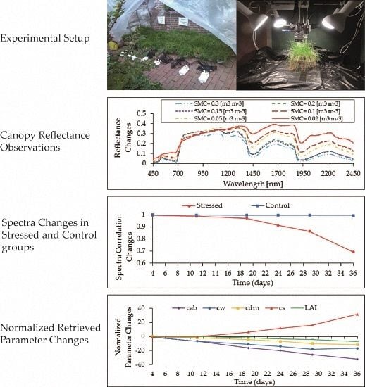
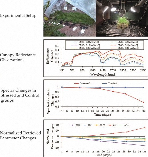
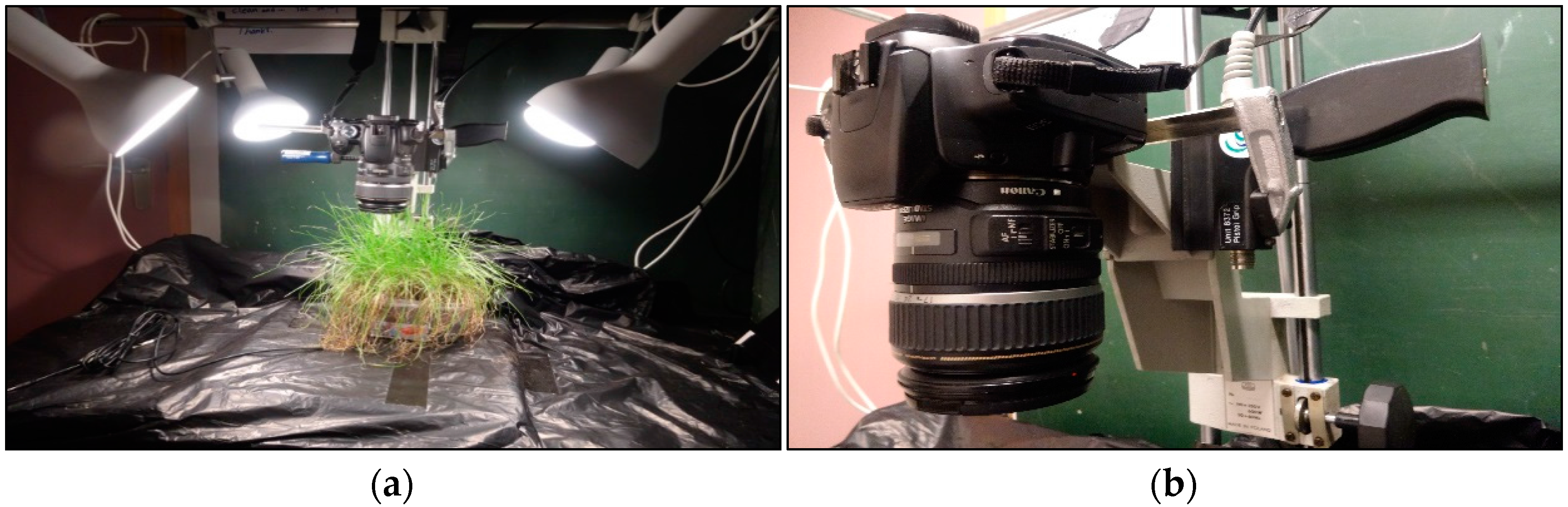
2.1. Experimental Design/Setup

A greenhouse experiment was conducted from 10 August 2014 until 27 October 2014 in the garden of the ITC Faculty of the University of Twente, the Netherlands. A commercially grown grass lawn (of Poa pratensis) was cut into 50 rectangles and transplanted into 21 cm × 14.5 cm pots with a depth of 12 cm, all filled with an organic soil. All 50 pots were watered regularly until the canopy height was about 15 cm (on 14 September 2014), after which they were placed in a greenhouse. The greenhouse shielded the vegetation from rainfall, but temperature, irradiance and humidity were not controlled. We selected grass for our experiments because of its rapid response to soil moisture deficits, and because the requirements for applying a 1-D turbid medium model like SAIL [28,29] are more easily met for relatively small canopies. The pots were divided into two equally sized groups: (1) a group under the well-watered condition and (2) a group that was not irrigated at all. Ten pots in each group were equipped with calibrated soil moisture sensors (Em50 Series, Decagon Devices, Inc., Hopkins Court Pullman, WA, USA). The well-watered pots were irrigated weekly with 200–250 mL water, such that the volumetric soil moisture content fluctuated around 30%–40%. The pots subject to no water treatment were not irrigated at all (started from 14 September 2014) to expose them to maximum water stress conditions. The greenhouse was fitted with removable plastic covers as walls, which were left open during daytime and closed during the night and rainfall events. Figure 1 shows the greenhouse setup for the experiment, plants in the groups and soil moisture sensors connected to the data loggers.

2.2. Instrumentation and Measurements

2.2.1. Canopy and Soil Spectral Measurements

Canopy spectra of all pots were measured in a dark room located in a remote sensing laboratory using the Analytical Spectral Devices (ASD), FieldSpec® 3 Hi-Res Portable Spectroradiometer in Full Range (ASD Inc., Boulder, CO, USA) that acquires continuous spectra in the VIS, NIR and SWIR regions (350 to 2500 nm). The plants were illuminated by four tungsten halogen quartz lamps of 100 W, each installed to be pointing in four azimuth directions, each under a 45° zenith incidence angle. These lamps were mounted about 80 cm above the plants (Figure 2a) to provide sufficient light to receive significant signal for accurate spectral measurements but without doing heat damage to the plant during the short measurement time. In this manner, we achieved a constant illumination. Measurements were done at the sampling intervals of the instrument (1.4 nm—VIS and NIR; 2 nm─SWIR) and were resampled by the instrument automatically into 1 nm intervals using linear and polynomial interpolations [45]. The fiber-optic cable was placed in a pistol and mounted on a stand (Figure 2b). In the setting, under 22.55 cm height and 25° field of view (FOV), the spectrometer scanned a diameter of 10 cm on the pot surface with the nadir point at the center of the circle. We made sure that the FOV of the sensor was fully covered by the plants. Every start of the measurements was preceded by a warming up time of the ASD for about 60 min (as recommended by the manuals). Before every target measurement, the ASD spectroradiometer was optimized for the illumination conditions using a spectralon white (BaSO4) reference panel. The ASD spectrometer was set to take 60 samples and compute the average value before storing these data (to reduce the noise in the spectral measurements). Each sample was transferred from greenhouse to the laboratory and placed in the measurement setup. After each measurement of spectral reflectance from the target sample pot, a photo was also taken by a digital camera (EOS 400D, Digital Rebel XTi, Melville, NY, USA) installed on the stand in the setup (Figure 2). Finally, the pot was moved back to the greenhouse.
Since the measurement of soil spectra is needed to be used as the background reflectance of the grass target samples in the radiative transfer model inversion [46], the reflectance of the background soil containing various values of soil moisture content was also measured. At the end of the experiment, the biomass of 10 samples was completely harvested to take soil reflectance measurements on a set of soil samples having a range of soil moisture (from dried soil to completely saturated soil). To measure volumetric soil moisture content of each sample, the pots were weighed in the laboratory both before and after drying (48 h, 45° Celsius), the difference being the mass of water originally in the sample. Then, volumetric soil moisture of soil samples was calculated by Equation (1):
θ v = θ g . ( ρ b ρ w )
where θv is volumetric soil moisture (m3·m−3), θg is gravimetric soil moisture (wet mass of soil—dry mass of soil/dry mass of soil) (g·g−1), ρb is soil bulk density and ρw is the density of water (g·cm−3).
In this experiment, in addition to canopy and soil reflectance measurements, some direct measurements of LAI and Cab of the grass were measured in the laboratory during the stress episode for model validation purposes. This enabled the comparison of the destructive laboratory measurements of parameters with corresponding parameters as retrieved from spectral readings. The measured parameters are described in the following subsection.

2.2.2. Leaf Area Index and Leaf Chlorophyll Content

LAI was measured directly during the experiment at different dates (having various soil moisture contents) by harvesting the pot samples which did not have a soil moisture sensor. Leaf area was measured at a representative sub-sample in the pot and related to its dry mass (oven dried at 65 °C for 48 h). To determine the leaf area, leaf samples were placed carefully on a sheet of paper and then were scanned with a flatbed scanner (the Xerox ColorQube 9301, Woerden, The Netherlands). The projected area was calculated using the ImageJ (the National Institutes of Health, Montgomery, AL, USA) software program. In all cases, we made sure that the leaves were not curled up or overlapping and tried to position the leaves to be as flat as possible in the position. We calibrated the area meter by using pieces of known area before measuring leaves and always checked that the whole leaves were positioned within the scanning area. The ratio of leaf area to leaf dry mass, known as specific leaf area [47], was calculated in cm2·g−1. Finally, the total dry mass of leaves collected within the pot surface area was converted into LAI by multiplying by the specific leaf area.
To take measurements of leaf chlorophyll content, we used the SPAD 502Plus leaf chlorophyll meter (Konica Minolta Sensing, Inc., Sakai, Osaka, Japan). We took ten chlorophyll samples from each pot during one measurement located in the field of view of the canopy reflectance measurements and used the average value. The relative values of the SPAD were converted into absolute amount of chlorophyll using a widely used calibration curve (Equation (2)) from the literature [48]:
C h l = 10 S 0.0265   R 2 = 0.94
where Chl is the absolute amount of chlorophyll in µmol·m−2 and S is the unitless value of the SPAD readings. Then, by considering the molecular mass of Chla and Chlb, unit conversions were made from μmol·m−2 to μg·cm2.

2.2.3. Visual Inspection

To monitor visible changes in the plants undergoing various treatments, we installed a digital camera on the stand (Figure 2) to take a photo of each sample after measurement of target spectral reflectance. In this manner, we could follow the changes of plant status over time by naked eye. The most important changes might be detected by visual observation including the decoloration of the leaves, the shape of the leaves and the openness of the canopy [15].

2.3. Spectral Acquisition

The grass spectra were measured six times during the experiment. There were ten pots in each measurement. In total, 108 spectra were collected in the stressed and control group. They were averaged to reduce noise and to enhance the representativeness of spectra for a specific day of measurement. As a result, six average spectra for the stressed and control group were investigated. To analyze the impacts of moisture deficit on different parts of the spectra, canopy spectral changes to different levels of moisture deficit during the experiment were plotted. To find the time of the first signs of stress in the reflectance spectra, we followed [15], and Pearson’s correlations were computed between the averaged spectra measured at the beginning and those of the measurements during the experiment over time, i.e., the other five averaged spectra, in each group. This indicated the degree of changes in the shape of the reflectance spectra over time. Afterwards, the ratio was computed between the averaged spectra measured at the beginning and those of the measurements during the experiment to find the relative changes as a function of the spectral position and time.

2.4. Water Stress-Related Vegetation Indices

Some of the widely used water stress-related vegetation indices were computed for the stressed and control group over time. Computed vegetation indices were categorized in three groups depending on the spectral information they use (Table 1). They can provide valuable information about water stress using just a few individual wavelengths. Normalized differences were found between the stressed and control groups for each of the computed indices. We performed a linear regression over the time series of the control group, then calculated the standard deviation of the residual of the data of the control group and the regression line, and used this standard deviation to normalize the differences between the two groups (control and stressed). The normalized values account for the variability in the control group. Selected vegetation indices were investigated during the drought episode to find the most sensitive indices for the stress detection in the early stages. A selection of the most promising spectral stress indices was made based on the literature.

2.5. Radiative Transfer Models (RTM) for Parameter Retrievals

Implementations of the well-known and widely used PROSPECT [44] and SAIL [28,29] radiative transfer models were selected for physically based leaf and canopy parameter retrieval. We used the RTMo model, which is a version of the four-stream SAIL model for the radiative transfer of incident light in canopies as used in the model SCOPE (Soil Canopy Observation of Photosynthesis and the Energy balance) [60,61]. RTMo is a combination of the “4SAIL” model [62], with a few additions, and the leaf radiative transfer model “Fluspect” which is basically the “PROSPECT5” model with a few modifications and additions. The main differences between RTMo (4SAIL + Fluspect) and PROSAIL (SAILH + PROSPECT4) are: (1) The leaf angle distribution in RTMo is described with two parameters—the mean leaf inclination parameter (LIDFa) and the bimodality of the leaf inclination distribution (LIDFb)—while PROSAIL uses only the Mean Leaf Inclination Angle (MLA); (2) the fraction of diffuse incoming solar radiation is spectrally dependt, whereas in PROSAIL it is considered as a constant value. Retrieval of canopy parameters from hyperspectral canopy level measurements was performed by inverting the RTMo model. The PROSPECT5 model [44,63] calculates the leaf hemispherical reflectance and transmittance as a function of four input parameters: (1) the leaf structural parameter N (unitless); (2) the leaf chlorophyll a + b concentration Cab (μg·cm−2); (3) the dry matter content Cdm (g·cm−2); and (4) the water concentration of the leaves Cw (g·cm−2). In Fluspect, also brown pigment concentration, i.e., Cs (arbitrary unit), is included. The 4SAIL model [28,29] is a one-dimensional bidirectional quasi-turbid medium radiative transfer model since leaf size is considered for the hot-spot effect. It defines the canopy as a horizontally homogeneous layer that consists of small, flat leaves. The model has been applied successfully to homogeneous vegetation canopies [14,28,64]. Like 4SAIL, RTMo includes the hot-spot effect. In addition to leaf reflectance and transmittance, the RTMo model requires some other input parameters to simulate the top-of-canopy bidirectional reflectance. These are the sun zenith angle, θs (deg); the sensor viewing angle, θo (deg); the relative azimuth angle between sensor and sun, ψ (deg); spectra of solar irradiance, Esun; sky irradiance, Esky, background reflectance (soil reflectance), rsl; LAI (m2·m−2); the hot-spot size parameter, defined as the ratio between the average width of the leaves and the canopy height [31], and the leaf inclination distribution function (LIDF).

2.6. Local Sensitivity Analysis of RTMo

By performing a sensitivity analysis for a model, the most (and least) important input parameters and, therefore, their roles in explaining the variance in the model output can be identified [65,66]. At the canopy level, local sensitivity analysis (LSA) was executed to find the influence of small changes in RTMo input parameters on different parts of the reflectance spectrum. In this study, LSA relies on the Jacobian J, which is the matrix of first partial derivatives of the relative model output. To improve the comparability of the various model parameters, the Jacobian was calculated by varying each parameter by 1% of its range and recording the corresponding reflectance difference. This reflectance difference equals:
Δ r = J P max P min 100
where J is the corresponding element of the Jacobian matrix. Pmax is the maximum and Pmin is the minimum value of input parameter P. To evaluate the influence of the parameters k over the entire spectrum and to find the most (and least) influential parameters, the indicator αk was defined as:
α k = 1 n i = 1 n J i , k 2

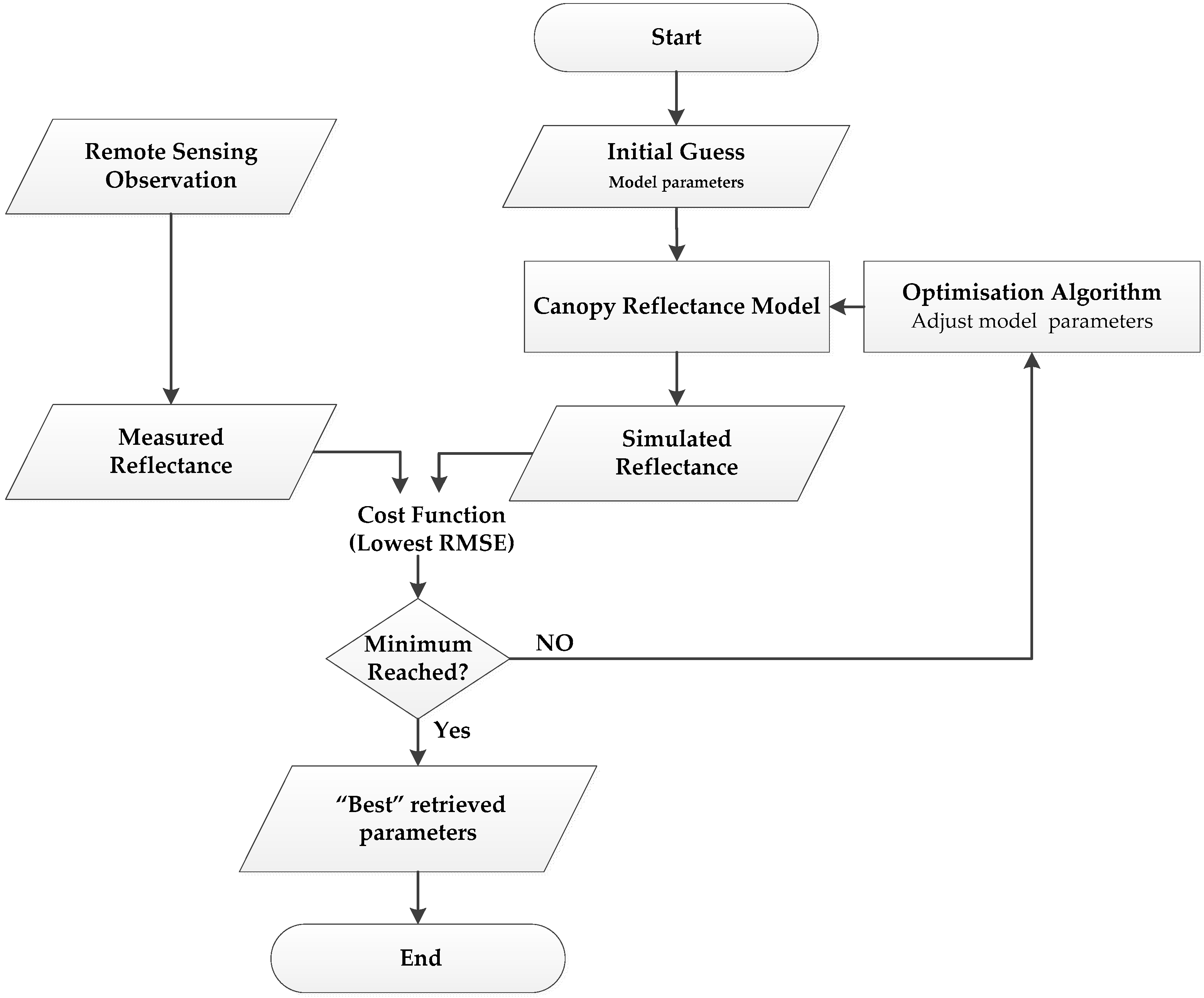
2.7. Inversion of RTMo

Inversion of a physical reflectance model aims at finding the set of input parameters which leads to the best match between simulated spectra by the model and observed spectra by the sensor. We used an iterative optimization technique for model inversion. This is a classical technique to invert any model with continuous variables which has been applied to invert radiative transfer models in remote sensing [67]. The iterative optimization technique searches for the best fit between the simulated and the measured reflectance spectra by iteratively running the canopy reflectance model (Figure 3) for different values of the input variables. The minimization of a cost function that accounts for the differences between the simulated and the measured reflectance spectra is used as a stopping criterion for this optimization problem. There are several studies that used different mathematical and statistical approaches to find the minimum [68].
Table 2 shows the initial guesses of input parameters used during the model inversion. To consider the contribution of the background soil reflectance in the model inversion, we changed the model soil spectra based on the value of soil moisture recorded in the pot for which canopy reflectance was taken.
The “Trust Region” algorithm implemented in the MATLAB (the MathWorks, Inc. Natick, MA, USA) function “lsqnonlin” was used to minimize the cost function. The cost function calculated was simply the sum of the squared differences over the whole wavelength range of the measured reflectance. From the result, the Root Mean Square Error (RMSE) between measured and simulated spectra was calculated. To avoid local minima, we did the minimization in numerous loops starting with various initial values. We changed the model initial values and simulated the canopy spectra. The results (data not shown) showed no significant effects of initial value choices on the retrieved parameters and the calculated RMSE between measured and simulated spectra.

2.8. Inversion Performance Evaluation (Statistics of Errors)

Table 3 presents a list of goodness-of-fit measures used in this research to indicate the agreement between simulated and observed values of LAI and Cab. Error indices (category 1 in Table 3) quantify the deviation of modeled from observed values. The statistics therefore describe the departure of model estimations from the one-to-one line [69]. The main advantage of calculating these error indices is that they represent the simple or squared differences between observed and simulated data. Correlation-based measures (category 2 in Table 3), have the advantage of being bounded (for R2 between 0 and 1), and, therefore, are independent of the unit of the parameter. The two most often used and traditional measures from category 1 and 2 (i.e., RMSE and R2, respectively) are often seen as insufficient for model validation purposes [69,70]. Instead, there are some dimensionless statistics (category 3) proposed in many studies, such as relative and normalized variations of the RMSE (i.e., RRMSE and NRMSE, respectively). The particular advantage of RRMSE and NRMSE is that the actual error can be calculated without being affected by the data unit.

3. Results

3.1. Visual Inspection

Grass responses to soil moisture deficit were tracked visually during the drought episode by analysis of their pictures. The visible signs of stress were increasing with time when moisture deficit progressed. The leaves turned from shiny to dull, decoloring to brown at the first signs of stress on day 10–11 of the experiment. Afterwards, by progress of stress, leaves started curling, shrinking, losing their color, allowing the brown leaves to dominate. At the end of the experiment in severe water stress, plants permanently wilted, all the leaves were discolored and the plants dried out completely and died.

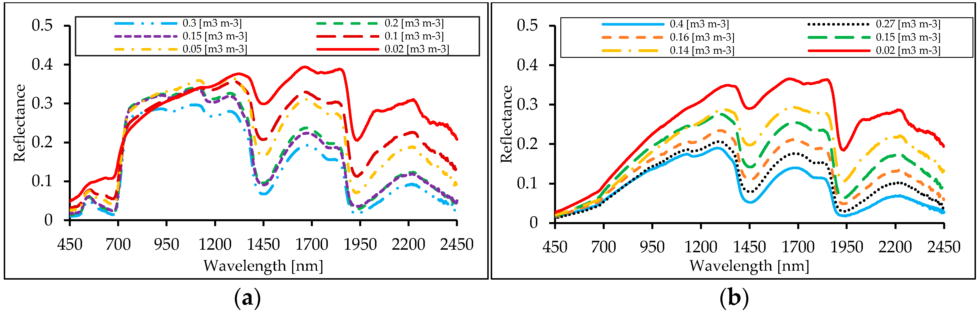
3.2. Shape of Reflectance Spectra

The changes in the shape of reflectance spectra for the selected grass, Poa pratensis, in response to the soil moisture deficit is illustrated in various ways. First, we visualized the effects of specific moisture deficit on the collected spectra to interpret the moisture-induced impacts on the shape of the reflectance curve on both canopy and soil from 450–2450 nm. Then, relative changes of the canopy reflectance values over time were analyzed to find the position and the time of the first sign of stress. Figure 4a shows selected measured spectra collected over the experiment in different soil moisture content. This result confirms that the stress affected all parts of the spectrum (either directly or indirectly) at the canopy level. Some parts of the spectrum, like 800–1100 nm, show a distinct decrease of reflectance values during the drought episode in case the plant is under stress (e.g., soil moisture contents 0.25, 0.2, 0.15, 0.10 and 0.05 m3·m−3). However, this is not the case under normal conditions in which the plant is not under stress (e.g., soil moisture contents ≥0.3, in the first days of the experiment). For instance, the reflectance in the region 800–1100 nm at a soil moisture of 0.02 m3·m−3 is lower than the canopy reflectance collected under other stress conditions (e.g., soil moisture contents 0.2, 0.15, 0.10 and 0.05 m3·m−3). The water absorption bands at 1450 and 1940 nm showed the strongest response by an increase of the reflectance. The visible green and visible red show smaller albeit distinct changes.
The spectra collected in the first stages of the drought episode (with soil moisture content of 0.3 (m3·m−3)) had low reflectance values in the visible part of the spectrum due to high concentrations of leaf chlorophyll. However, a decrease in chlorophyll concentration as a result of water stress increased the visible reflectance. Canopy reflectance of vegetation also depends on the reflectance properties of the underlying soil [71]. Figure 4b illustrates how soil reflectance changed due to different soil moisture contents in the experiment.
To find the time when the first drought-induced changes take place, we computed Pearson’s correlation (as in [15]) between the mean spectrum taken at the beginning of the experiment and those of the measurements during the experiment over time in both stress and control treatments (Figure 5a). Values smaller than 1.0 indicate that the shape of the spectral curve changed compared to the first measurement taken at the beginning of the experiment in the stressed and control groups. This analysis showed that on 17 September 2014 the first sign of stress occurred since the reflectance of Poa pratensis started deviating from the first measurement as early as day 4 and, therefore, the correlation of the stressed group started declining at this time. To identify the spectral position in which the first signs of stress could be detected, we calculated the ratio between reflectance values collected at day 11 and day 4 for the stress group expressed as a percentage change (Figure 5b). The first considerable responses could be seen at the major water absorption bands, especially at 1930 nm (62%) and 1440 nm (29%). Furthermore, distinct changes were detected around 550–700 nm with a maximum at 675 nm (31%). However, the minor water absorption bands around 970 nm and 1200 nm did not show different responses from the surrounding wavelengths and were not recognizable in the graph.

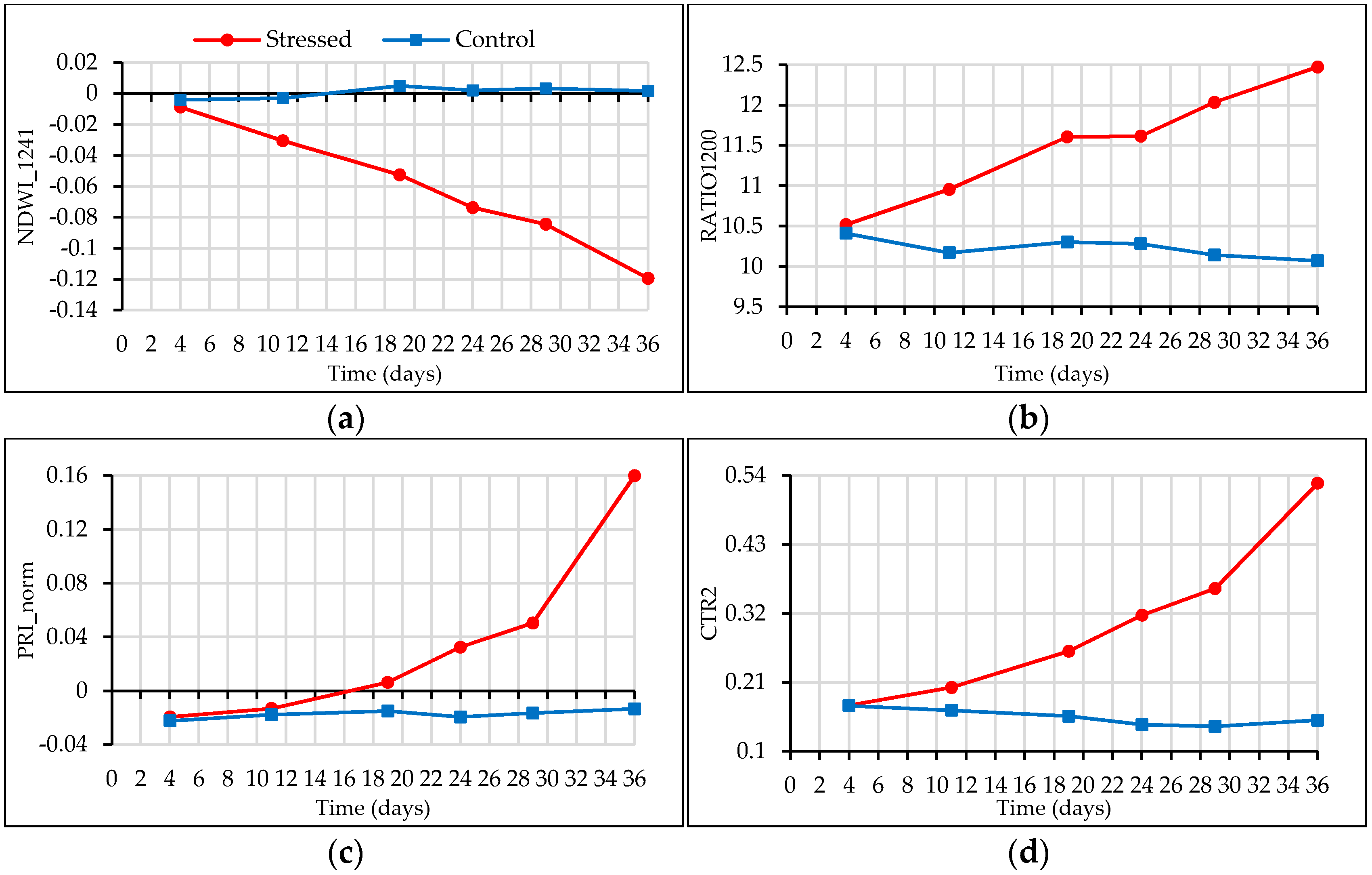
3.3. Spectral Indices

To find the most sensitive spectral indices for detection of water stress in the early stages, we computed the widely used indices related to water stress. The selected indices showed different behaviors over time during the experiment. The normalized differences of the index values in the stressed group compared to the control group are displayed in Figure 6. To find the normalized differences of the index values, first a linear regression was performed over the time series of the control group. Second, the standard deviation of the residual of the data of the control group with respect to the regression line was calculated, as a measure for the variability in the control group. This standard deviation was used to normalize the differences between the two groups (control and stressed). The threshold of two times the response of the control group, suggested in previous studies [15], was used to decide whether the stress index actually detected the stress or not. Based on this threshold, the majority of selected indices could detect the stress in the early stages (Figure 6a). The results showed that the NDWI_1241 was the best stress detector by exceeding the threshold. The response of the NDWI_1241, RATIO1200, BGI2 and NDWI_2130 were 10, 8.7, 8.6 and 8.2 times stronger for the stress group than for the control group, respectively (Figure 6a).
The MSI, NDII, NWI_1, and WBI indices also showed a stronger response (greater than six times the one of the control group) to the stress in the early stages. However, PRI_norm showed no detectable response to the stress since its response stayed below the defined threshold. The vegetation indices responses to long-term stress, at the end of the experiment, showed that all of the selected indices detected the stress (Figure 6b). The results showed that the PRI_norm was the best detector of long-term stress conditions. The response of the PRI_norm, CTR2, BGI2 and NDWI_1241 to long-term stress were 76, 53, 51 and 44 times stronger for the stress group than for the control group respectively (Figure 6b). Figure 7a,b shows the development over time for the two best-performing stress indices (NDWI_1241 and RATIO1200) in response to short-term stress (at day 11). Figure 7c,d shows the development over time for the two best-performing stress indices (PRI_norm and CTR2) in response to long-term stress (at day 36). As expected, indices in the control group did not change over time, except for small variations that might be explained by the noise level of the index [15].
NDWI_1241, the best performing index for short-term stress (at day 11) showed a downward trend over time during the experiment, whereas RATIO1200, PRI_norm and CTR2 showed upward trends. In addition, we found that BGI2 and NDWI_1241 had detectable and strong responses for both short-term and long-term stress.

3.4. RTMo (4SAIL + Fluspect) Radiative Transfer Modeling

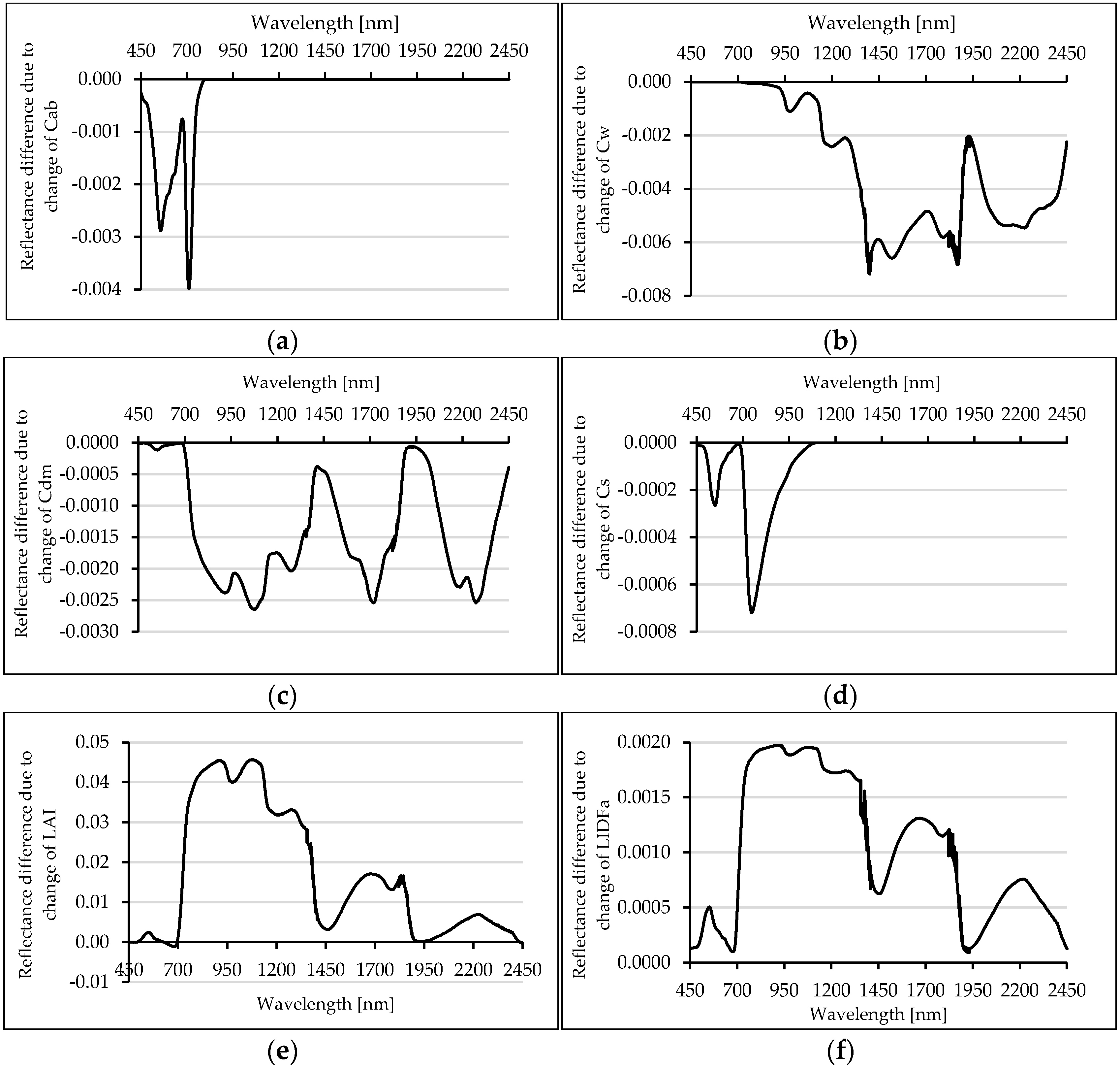
3.4.1. RTMo Sensitivity Analysis Results

We changed all the parameters (Cab, Cdm, Cw, Cs, LAI, and LIDFa) by 1% of their total range and then determined the reflectance differences (Figure 8). This shows the influence of each parameter in a comparable way. The normalized derivative demonstrated two clearly indicated peaks in the reflectance response to Cab change at 557 nm and 710 nm (Figure 8a). The second peak was the most sensitive one of the entire spectrum and the visible region was indicated as the most sensitive to Cab change. In contrary, the small variation in Cw was expressed most strongly in the SWIR (Figure 8b). The greatest sensitivity to variation in Cw was exhibited at 1400, 1870, 1516, 2225 nm. Variation in Cw also contributes significantly in the NIR, especially at 1198 and 976 nm. Variation in the Cdm was expressed most strongly in both the NIR and the SWIR (Figure 8c). It showed pronounced peaks at 916, 1075, 1272, 1719, 2182 and 2273 nm. Two clearly indicated peaks are observed in the reflectance response to Cs change at 551 nm and 748 nm. However, the NIR and SWIR parts did not respond to changes of the Cs parameter (Figure 8d). Although variations in LAI and LIDF triggered the reflectance response at similar spectral wavelengths (910, 1081, 1279, 1681, 1827 and 2221 nm), the LIDF response was quite weak compared to the one of LAI (Figure 8e,f).
The computed αk values (Table 4) showed that the most influential parameters over the entire spectrum were LAI and Cw with αLAI and αCw values of 0.0231 and 0.0039. Thus, by having a small change in these parameters, the reflectance will respond relatively stronger in comparison to the other ones. The least influential parameters identified were Cab and Cs.

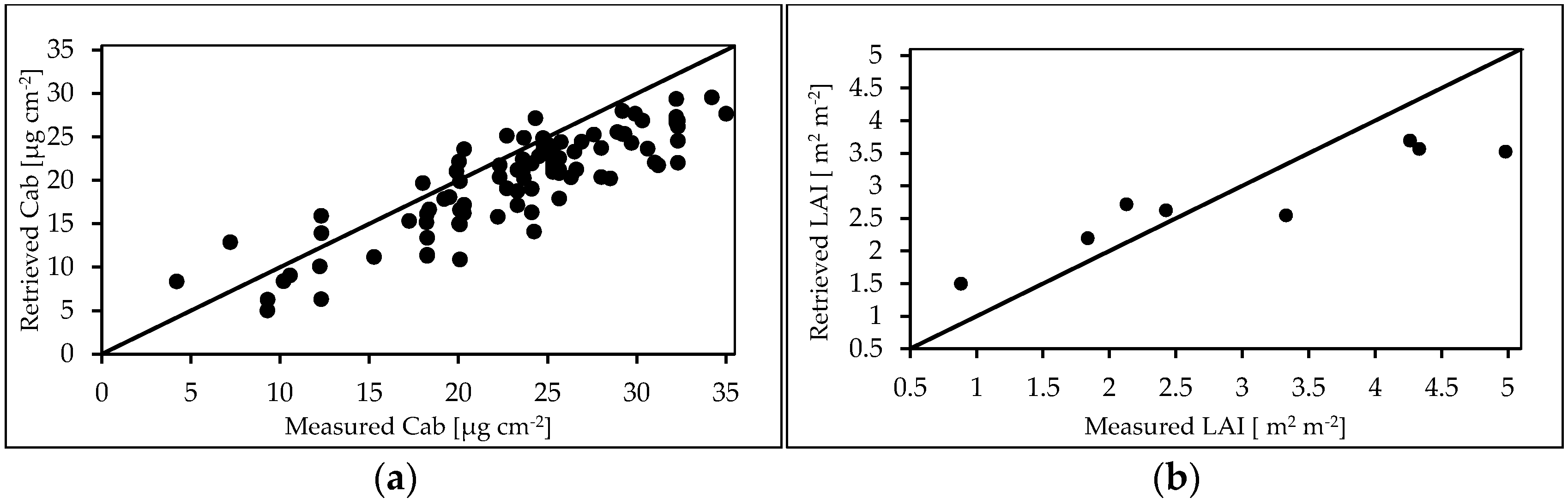
3.4.2. RTMo (4SAIL+Fluspect) Inversion Results

The RMSE of measured and simulated spectra was employed as the criterion of the model inversion performance. Figure 9a,b shows the difference between two simulated and measured canopy spectra on different days (day 11 and 36) of the experiment. These examples represent the performance of the inversion since good quality of spectral fit achieved. Furthermore, the distribution of RMSE between measured and simulated canopy reflectance spectra during the drought experiment for all simulations (under various soil moisture conditions) is presented in Figure 9c. The small error in the model inversion (0.002 < RMSE < 0.009) showed that the model was able to accurately reproduce the observed reflectance spectra under different soil moisture contents during the experiment.
In addition, the inversion results were also evaluated in their accuracy (deviations from the measured parameter values). In Figure 10, the retrieved and measured LAI (n = 8) and Cab (n = 108) are illustrated in the form of scatter plots and deviations from the one-to-one line.
For the retrieved and measured properties, statistical measures were calculated. Varying statistical performances are given for the two variables (i.e., LAI and Cab; Table 5). RMSE and R2 calculated 0.75 (m2·m−2), 0.87 for LAI and 4.61 (µg·cm−2), 0.74 for Cab estimation. Because of the different units, we also calculated NRMSE and RRMSE, which are dimensionless and suitable indices for comparisons between LAI and Cab variables. The calculated NRMSE (LAI: 0.18, Cab: 0.15) and RRMSE (LAI: 24.8%, Cab: 19.8%) are presented in Table 5.

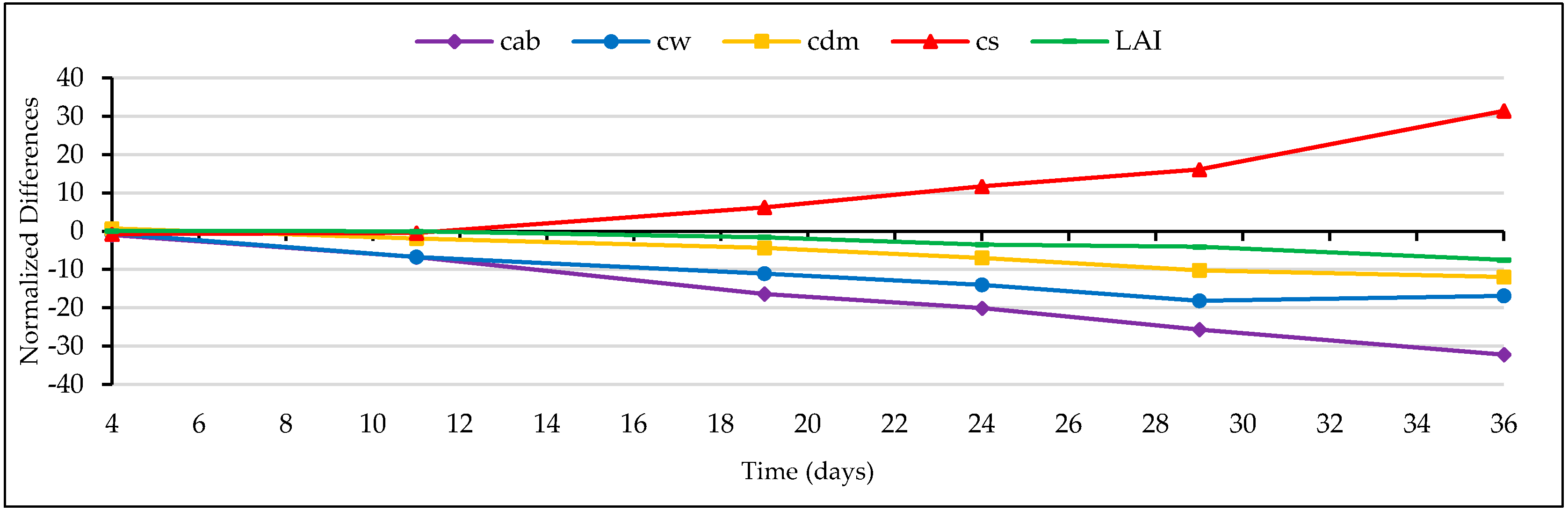
3.4.3. Trend of the Retrieved Grass Properties

Retrieved parameters were plotted against soil moisture and time during the experiment in Figure 11. This way, we could follow the trend of changes and detect water stress impacts on the retrieved parameters. As can be seen from the left panels of Figure 11, the relationship between retrieved parameters and soil moisture content is nonlinear. Thus, just to guide the eye and keep it fairly simple, we fitted a second order polynomial curve. Although using higher degrees (third or fourth order function) can provide a better fit, we avoided using them for the sake of stability. The retrieved grass parameters co-varied with soil moisture content (Cab: R2 = 0.76 and RMSE = 3.58, Cw: R2 = 0.70 and RMSE = 0.001, Cs: R2 = 0.69 and RMSE = 0.06, Cdm: R2 = 0.40 and RMSE = 0.001, LAI: R2 = 0.45 and RMSE = 0.48). In the right panels (of Figure 11) we show the parameter changes over time in separated stressed and control groups derived from the averaged spectra of all measurements from the same day. In almost all cases, the value of the control group displayed, as expected, a horizontal course indicating that vegetation parameters did not change much during the measurement period. However, water stress affected all grass parameters in the stressed group during the drought episode. The maximum value retrieved for the leaf chlorophyll content at the first measurement (day 4) was about 22 (ug·cm−2), which then decreased during the experiment and reached the minimum value of 3.6 on the last measurement (day 36). Leaf water content changed from 0.006 to 0.001 (g·cm−2) from the beginning of the experiment to the end. Although the leaf dry matter content showed a different behavior in the stressed group compared to that of control, its value at the end of the drought episode of 0.0015 (g·cm−2) was similar to the value at the beginning of 0.0017 (g·cm−2). Following the response of Cs to the stress over time showed a different trend in comparison to the other parameters since it deviated away from the horizontal control line upward. The minimum value for Cs was retrieved on day 4 while the maximum value recorded at the end of experiment on day 36. LAI responded to the stress during the experiment and decreased from 2.3 (m2·m−2) at the beginning to 1.5 (m2·m−2) at the end of the experiment. In addition, the results showed that LAI and Cs responded to the stress relatively late (after day 11) compared to the other parameters such as Cw and Cab which responded in the early stages (day 4).
To compare the effects of stress on various parameters and detect the order of grass responses during the experiment, we normalized the differences for each of the parameters between the stressed and the control group. The normalized values account for the variability in the control group.
The relative changes of the parameters in early stages of the stress (Figure 12) demonstrate that the first effects of stress on the grass parameters are the change of Cw and Cab, followed by Cdm and Cs. These parameters started responding to stress in the earlier stages of stress. LAI and Cs did not respond to the stress until 15 days after the start of the experiment. Almost all grass parameters responded to the stress at the end of the experiment. The strongest response at the end of the experiment compared to the control group was the change of Cs, followed by Cab, Cw, Cdm and LAI, respectively.

4. Discussion

We conducted a drought experiment to follow water stress impacts on grass reflectance and properties over time. This experiment lasted for 80 (35 + 36 + 9) days. In the first 35 days, all plants were watered regularly until the canopy height was about 15 cm and the maximum growth reached. In the next 36 days, the canopy spectral measurements were collected in the stressed and control group. In addition, some measurements of LAI (n = 8) and Cab (n = 108) were taken. In the last nine days, soil reflectance measurements under various moisture conditions were taken. After the experiment, all of the plants ultimately died except for the control group.

4.1. Visual Interpretation of the Stress Effects

The visible signs of stress on the plants, including curling and shrinking of the leaves, becoming fragile, turning from shiny to dull and finally some leaves decoloring, were observed first after 10–11 days from the start of the drought. From day 19 onwards the proportion of dry leaves increased rapidly. The visible signs of stress were increasing by the time the moisture deficit progressed. This confirms other studies revealing similar results. For instance, De Jong et al. [15] reported the first visible sign of different stresses (water saturation, light deprivation, water deprivation, heat and chlorine poisoning) for Buxus sempervirens on average after 15 days for all stresses and after 13 days for water deprivation [15]. They also found that the analysis of the infrared photos collected during the stress did not provide additional information after the visual inspection of the plants. An interpretation of the canopy reflectance responses to soil moisture deficit revealed that the stress affected all parts of the spectrum. In particular, changes were detected in the 450–700 nm and 1300–2500 nm ranges (Figure 4), which can be explained by the role of the concentrations of pigments and water, respectively. These findings are in full agreement with Carter [72], Zarco-Tejada et al. [73] and Chavez et al. [24], who demonstrated two effects of water stress on the reflectance spectra; direct (primary) effects and indirect (secondary) ones. ”Direct effects” are the primary impacts of water stress (dehydration) on vegetation which resulted solely from the spectral properties of water (this gives changes of the reflectance in the range of 1300–2500 nm because of less absorption by water). The “indirect effects” are secondary impacts that could not be explained solely by the spectral properties of water (manifested by changes of the reflectance in the range of 400–700 nm because of more cell wall–air interfaces within the leaf tissue as well as the effect of dehydration on the concentrations of pigments. Canopy spectral reflectance in the near-infrared (NIR) region (750–1300 nm) initially increased but, in later stages of water stress, it decreased. This pattern can be explained by the consequence of the deterioration of cell walls [74], loss of leaves and the changes in LIDF [75]. Our findings of NIR responses to water stress support previous studies [24,34,57]. We observed that the percentage of “direct effects” (24%) in the early stages of the stress (after 11 days being under stress) were more than “indirect effects” (17%). However, in the last stages of the stress (after 36 days being under stress) the percentage of “indirect effects” (171%) were more than “direct effects” (146%).

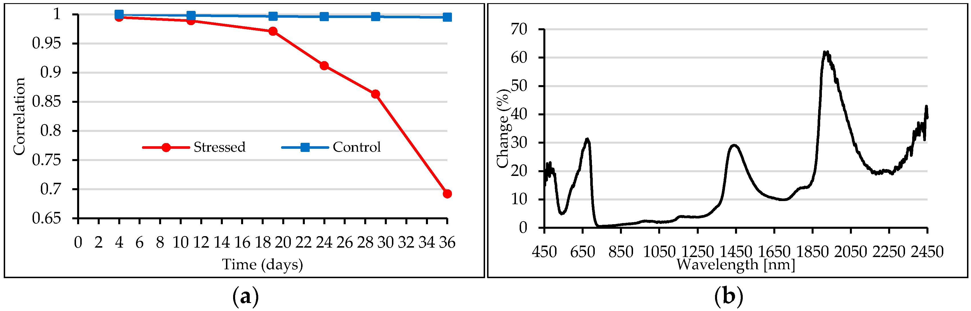
4.2. First Sign of the Stress

The analysis of the collected spectra over time showed that the first considerable responses could be seen near the major water absorption bands specially at 1930 nm and 1440 nm (Figure 5b). In addition, distinct changes were detected around 550–700 nm with a peak value located at 675 nm. We did not detect significant changes at the location of the minor water absorption bands at 970, 1200, and 1770 nm, which is in agreement with previous studies [15]. Based on Pearson’s correlation analysis, the correlation of the stressed group started declining from day 4, thereby showing the first sign of the stress visible in the spectra. Pearson’s correlation computation between the spectra proved a valuable way to detect subtle spectral changes and to identify the moment in time of the stress-induced spectral changes of the plant. The spectroscopic signs of stress were detectable six days before the visible signs. The conclusion is that the use of spectroscopic techniques allows a much earlier detection of plant stress than visible inspection.

4.3. Water Stress-Related Vegetation Indices

The spectral stress indices that best illustrated the stress effects in the earlier stages in our experiment were the NDWI_1241 and RATIO1241. These two spectral indices, using the reflectance in SWIR and NIR around 857, 1241, 1180–1220, 1090–1110, 1265–1285 nm, were the most sensitive ones among the examined indices. This is in agreement with Ceccato et al. [58] who concluded that a combination of SWIR and NIR is necessary to improve the accuracy in estimating vegetation water content at the leaf level from optical observations. Our study showed that the response of the NDWI_1214 index was ten times as strong for the stress group as for the control in the early stages of the stress. This index is a measure of liquid water molecules in vegetation canopies that interacted with the incoming solar radiation. This is in agreement with Gao [53] who demonstrated the sensitivity of NDWI to the total amounts of liquid water in stacked leaves. He explained the reasons of sensitivity of NDWI by the location of the selected channels, their negligible or weak absorption properties and less sensitivity to atmosphere effects, although atmospheric effects are not relevant in the present study. The spectral indices that best illustrated the development of water stress over time during the experiment were PRI_norm and CTR2. PRI_norm is normalized by both structure and by the red edge chlorophyll-related index. Zarco-Tejada et al. [27] concluded that PRI_norm is a more linearly related index for reading canopy chlorophyll content levels than the standard PRI index, due to its good performance. CTR2 uses the wavelength 760 (NIR shoulder) in combination with a spectral band in the red edge at 695 nm, which is sensitive to chlorophyll, to compute the index value. Our results match other studies which identified CTR2 as one of the best stress indicators [15,76,77].

4.4. RTMo Sensitivity Analysis

Local sensitivity analysis provided useful insights about the parameter changes’ influences on the simulated reflectance. The results showed the ability of the RTMo model to link variations of reflectance to variations of grass parameters. Small changes in Cw resulted into strong responses in the SWIR part of the spectrum. The importance of Cw in accounting for variance in the SWIR supports previous studies [23,58,78]. The variation in Cdm showed significant responses in the SWIR and NIR part. This is in agreement with other studies as well [66,79]. The main cause of the strong response in the NIR part might be explained by the absorption of Cdm since it is the only absorber in most of the NIR region and tends to increase with the age of the leaf [80]. The response of reflectance to a small variation in LAI and LIDF was detected at similar wavelengths in the NIR and SWIR. This is in agreement with other studies which reported similar effects of LAI and LIDF in PROSAIL model sensitivity analysis [64] and the LIDF as the main variable influencing the relationship between vegetation indices and LAI [81]. Reflectance in the green (557 nm) and red edge (710 nm) responded clearly to changes of Cab. This result confirms other studies explaining the relationship between reflectance and Cab [82].

4.5. RTMo Parameter Retrieval

A physical approach was adopted in this research to retrieve grass parameters from spectroradiometer measurements. This has many advantages, as it is based on physical laws, use of all spectral bands, the least reliance on in situ measurements and it gives generalizable results, just to name a few [43,83]. However, use of this approach (i.e., radiative transfer models) is more complex than a simple statistical method (i.e., vegetation indices). Several studies have demonstrated that vegetation parameter retrieval using radiative transfer models yields more accurate results compared to that of vegetation indices. For instance, Atzberger et al. [83] compared physical and statistical-based retrieval methods to map grassland LAI using airborne imaging spectroscopy. They concluded that RTM inversion based on a look-up table approach and predictive equations yields a higher accuracy with a normalized RMSE of 0.18 and 0.38 respectively for LAI estimation. In our experiment, although we inverted the RT model by means of an optimization algorithm, the results for LAI retrieval are in good agreement with the findings of Atzberger et al. [83]. The calculated normalized RMSE for LAI retrieval in our experiment is 0.18 (Table 5) which is in full agreement with their studies.
Simulated spectra fitted well with measured spectra collected at different soil moisture deficit conditions during the drought experiment. Low RMSE between measured and simulated spectra (ranging from 0.002 to 0.009) for a variety of soil moisture conditions confirmed that the inversion was successful. We conclude that there was a positive significant relationship between retrieved and measured parameters. Nevertheless, the variation in parameters, (i.e., the range of values) especially in Cab, showed that retrieved values had a smaller range than the destructive measurements. This might be explained by two facts: (1) the RTMo model uses one Cab value for all leaves in the pot, but measurements taken from individual leaves are more variable; and (2) to convert the relative values of the measured chlorophyll by SPAD 502 into the absolute values we used a calibration curve from the literature [48]. Changes of Cw and Cab were found as the first signs of stress on vegetation parameters. Other researchers concluded that changes in canopy reflectance due to water stress were mostly explained by equivalent water thickness and LAI [24]. We found that all vegetation parameters responded to stress at the end of the experiment. The strongest response at the end of the experiment compared to the control group was the change of Cs, followed by Cab, Cw, Cdm and LAI. Our experiment shows that soil moisture deficit stress impacts can be tracked in a drought episode over time. Spectroscopy is a valuable technique to detect stress effects on the reflectance spectra in an early stage.

5. Conclusions

In this study, we investigated in the laboratory the grass response to water stress in a Poa pratensis canopy exposed to various levels of soil moisture deficit. We used spectroscopic techniques, to observe the stress impacts on canopy reflectance, and Radiative Transfer Model (RTM) inversion, to detect stress effects on grass properties. These techniques have the promising potential of detecting the drought-induced effects on grass reflectance and properties during a drought episode. Sensitivity analysis of RTMo (RTM of solar and sky radiation) simulated reflectance to a small change of its input parameters shows that changes in Leaf Area Index (LAI), leaf water content (Cw) and leaf dry matter (Cdm) trigger a stronger response in the reflectance compared to the other parameters. Spectral analysis shows that short-term moisture deficit stress results in changes of 17% in reflectance values in the visible part (450–700 nm), of 2.3% in the near-infrared (NIR) part (700–1300 nm), and of 23.7% in the short-wave infrared (SWIR) part (1300–2450 nm). However, long-term stress results in changes of 170% in reflectance values in the visible part, of 9.3% in the (NIR) part, and of 146% in the SWIR part. The RTMo inversion shows that Cw, leaf chlorophyll content (Cab) and Cdm respond strongly to short-term moisture-deficit stress, while LAI and senescent material (Cs) changes are the main responses of vegetation to long-term stress. Spectral measurements allow moisture stress detection up to six days earlier than visual naked-eye observations. The first spectral signs of stress are detectable near the major water absorption bands. Among grass properties, the first signs of moisture stress are changes of Cw and Cab. The most promising water stress-related vegetation indices for early stress detection are NDWI_2130 and MSI since their responses to the stress are significantly stronger in the early stages for the stress group. In addition, for the entire drought episode, PRI_norm and CTR2 are identified as the best ones for stress detection. By the time it displays visible symptoms of stress, a plant can already be adversely affected. This research demonstrated that spectroscopic techniques and RTMo inversion allow presymptomatic monitoring (early detection) of changes in the canopy reflectance and biophysical properties non-destructively. Beyond the scale and plant species of this study, it is unclear how broadly applicable this approach will be and to what extent these findings could be generalized, since this would require applying the proposed approach in the “real world” using satellite observations. It is currently under investigation by the authors to upscale the results obtained in this study to field conditions. We expect that spectral analysis and the RTMo model inversion against satellite images would enable the detection of water stress impacts on vegetation properties in the ecosystem. Using these for crop monitoring would allow us to alleviate stress at an early stage, thus avoiding irreversible damage and substantially reducing yield losses.

Acknowledgments

We are very grateful to Marijke van der Tol and Josip Završki who gave us generous help during the laboratory measurements, particularly during all the sampling conducted in the laboratory. Also, we would like to acknowledge all the support received from the ITC Geoscience and Remote Sensing Laboratory staff, especially Boudewijn de Smeth, Watse Siderius and Murat Uçer. The authors would like to thank three anonymous reviewers for their constructive comments and suggestions to improve the quality of the paper.

Author Contributions

All authors have made major and unique contributions in this research. The main idea of the study was conceived by Bagher Bayat and then further developed with the help of Wouter Verhoef’s and Christiaan van der Tol’s scientific advice and comments. Bagher Bayat, Christiaan van der Tol and technicians (see Acknowledgements) set up the experiment and the laboratory design. Spectral data collection, destructive measurements, data analysis, model inversion, simulation and interpretation of the results were performed by Bagher Bayat. The code for the iterative optimization was developed by Christiaan van der Tol and Bagher Bayat. All authors discussed the results and commented on the manuscript at all stages. The original manuscript was written by Bagher Bayat and then polished and revised by Christiaan van der Tol and Wouter Verhoef.

Conflicts of Interest

The authors declare no conflict of interest.

References

  1. Reddy, A.R.; Chaitanya, K.V.; Vivekanandan, M. Drought-induced responses of photosynthesis and antioxidant metabolism in higher plants. J. Plant Physiol. 2004, 161, 1189–1202. [Google Scholar] [CrossRef]
  2. Zhang, Y.; Peng, C.H.; Li, W.Z.; Fang, X.Q.; Zhang, T.L.; Zhu, Q.A.; Chen, H.; Zhao, P.X. Monitoring and estimating drought-induced impacts on forest structure, growth, function, and ecosystem services using remote-sensing data: Recent progress and future challenges. Environ. Rev. 2013, 21, 103–115. [Google Scholar] [CrossRef]
  3. Lidon, Z.Z.; Cebola, F. An overview on drought induced changes in plant growth, water relations and photosynthesis. Emirates J. Food Agric. 2012, 24, 57–72. [Google Scholar] [CrossRef]
  4. Wolf, S.; Eugster, W.; Ammann, C.; Häni, M.; Zielis, S.; Hiller, R.; Stieger, J.; Imer, D.; Merbold, L.; Buchmann, N. Contrasting response of grassland versus forest carbon and water fluxes to spring drought in Switzerland. Environ. Res. Lett. 2013, 8, 035007. [Google Scholar] [CrossRef]
  5. Laio, F.; Porporato, A.; Fernandez-Illescas, C.; Rodriguez-Iturbe, I. Plants in water-controlled ecosystems: Active role in hydrologic processes and response to water stress II. Probabilistic soil moisture dynamics. Adv. Water Resour. 2001, 24, 745–762. [Google Scholar] [CrossRef]
  6. Larcher, W. Physiological plant ecology: Ecophysiology and stress physiology of functional groups. Springer Science & Business Media: New York, NY, USA, 2003. [Google Scholar]
  7. Earl, H.J.; Davis, R.F. Effect of drought stress on leaf and whole canopy radiation use efficiency and yield of maize. Agron. J. 2003, 95, 688–696. [Google Scholar] [CrossRef]
  8. Dorman, M.; Perevolotsky, A.; Sarris, D.; Svoray, T. The effect of rainfall and competition intensity on forest response to drought: Lessons learned from a dry extreme. Oecologia 2015, 177, 1025–1038. [Google Scholar] [CrossRef] [PubMed]
  9. Dorman, M.; Svoray, T.; Perevolotsky, A.; Sarris, D. Forest performance during two consecutive drought periods: Diverging long-term trends and short-term responses along a climatic gradient. For. Ecol. Manag. 2013, 310, 1–9. [Google Scholar] [CrossRef]
  10. Zhao, X.; Wei, H.; Liang, S.; Zhou, T.; He, B.; Tang, B.; Wu, D. Responses of natural vegetation to different stages of extreme drought during 2009–2010 in Southwestern China. Remote Sens. 2015, 7, 14039–14054. [Google Scholar] [CrossRef]
  11. Chaerle, L.; Van Der Straeten, D. Seeing is believing: Imaging techniques to monitor plant health. Biochim. Biophys. Acta—Gene Struct. Expr. 2001, 1519, 153–166. [Google Scholar] [CrossRef]
  12. Fedotov, Y.; Bullo, O.; Belov, M.; Gorodnichev, V. Experimental Research of Reliability of Plant Stress State Detection by Laser-Induced Fluorescence Method. Int. J. Opt. 2016, 2016, 6. [Google Scholar] [CrossRef]
  13. Barton, C.V.M. Advances in remote sensing of plant stress. Plant Soil 2011, 354, 41–44. [Google Scholar] [CrossRef]
  14. Meroni, M.; Colombo, R.; Panigada, C. Inversion of a radiative transfer model with hyperspectral observations for LAI mapping in poplar plantations. Remote Sens. Environ. 2004, 92, 195–206. [Google Scholar] [CrossRef]
  15. De Jong, S.M.; Addink, E.A.; Hoogenboom, P.; Nijland, W. The spectral response of Buxus sempervirens to different types of environmental stress—A laboratory experiment. ISPRS J. Photogramm. Remote Sens. 2012, 74, 56–65. [Google Scholar] [CrossRef]
  16. Suárez, L.; Zarco-Tejada, P.J.; Berni, J.A.J.; González-Dugo, V.; Fereres, E. Modelling PRI for water stress detection using radiative transfer models. Remote Sens. Environ. 2009, 113, 730–744. [Google Scholar] [CrossRef]
  17. Ustin, S.L.; Gitelson, A.A.; Jacquemoud, S.; Schaepman, M.; Asner, G.P.; Gamon, J.A.; Zarco-Tejada, P. Retrieval of foliar information about plant pigment systems from high resolution spectroscopy. Remote Sens. Environ. 2009, 113, S67–S77. [Google Scholar] [CrossRef] [Green Version]
  18. Serbin, S.P.; Singh, A.; McNeil, B.E.; Kingdon, C.C.; Townsend, P.A. Spectroscopic determination of leaf morphological and biochemical traits for northern temperate and boreal tree species. Ecol. Appl. 2014, 24, 1651–1669. [Google Scholar] [CrossRef]
  19. Serbin, S.P.; Singh, A.; Desai, A.R.; Dubois, S.G.; Jablonski, A.D.; Kingdon, C.C.; Kruger, E.L.; Townsend, P.A. Remotely estimating photosynthetic capacity, and its response to temperature, in vegetation canopies using imaging spectroscopy. Remote Sens. Environ. 2015, 167, 78–87. [Google Scholar] [CrossRef]
  20. Asner, G.P.; Nepstad, D.; Cardinot, G.; Ray, D. Drought stress and carbon uptake in an Amazon forest measured with spaceborne imaging spectroscopy. Proc. Natl. Acad. Sci. USA 2004, 101, 6039–6044. [Google Scholar] [CrossRef] [PubMed]
  21. Coates, A.R.; Dennison, P.E.; Roberts, D.A.; Roth, K.L. Monitoring the impacts of severe drought on southern California Chaparral species using hyperspectral and thermal infrared imagery. Remote Sens. 2015, 7, 14276–14291. [Google Scholar] [CrossRef]
  22. Verrelst, J.; Schaepman, M.E.; Koetz, B.; Kneubühler, M. Angular sensitivity analysis of vegetation indices derived from CHRIS/PROBA data. Remote Sens. Environ. 2008, 112, 2341–2353. [Google Scholar] [CrossRef]
  23. Ceccato, P.; Gobron, N.; Flasse, S.; Pinty, B.; Tarantola, S. Designing a spectral index to estimate vegetation water content from remote sensing data: Part 2. Validation and applications. Remote Sens. Environ. 2002, 82, 198–207. [Google Scholar] [CrossRef]
  24. Chávez, R.O.; Clevers, J.G.P.W.; Herold, M.; Ortiz, M.; Acevedo, E. Modelling the spectral response of the desert tree Prosopis tamarugo to water stress. Int. J. Appl. Earth Obs. Geoinf. 2013, 21, 53–65. [Google Scholar] [CrossRef]
  25. Houborg, R.; Soegaard, H.; Boegh, E. Combining vegetation index and model inversion methods for the extraction of key vegetation biophysical parameters using Terra and Aqua MODIS reflectance data. Remote Sens. Environ. 2007, 106, 39–58. [Google Scholar] [CrossRef]
  26. Darvishzadeh, R.; Atzberger, C.; Skidmore, A.; Schlerf, M. Mapping grassland leaf area index with airborne hyperspectral imagery: A comparison study of statistical approaches and inversion of radiative transfer models. ISPRS J. Photogramm. Remote Sens. 2011, 66, 894–906. [Google Scholar] [CrossRef]
  27. Zarco-Tejada, P.J.; González-Dugo, V.; Williams, L.E.; Suárez, L.; Berni, J.A.J.; Goldhamer, D.; Fereres, E. A PRI-based water stress index combining structural and chlorophyll effects: Assessment using diurnal narrow-band airborne imagery and the CWSI thermal index. Remote Sens. Environ. 2013, 138, 38–50. [Google Scholar] [CrossRef]
  28. Verhoef, W. Light scattering by leaf layers with application to canopy reflectance modeling: The SAIL model. Remote Sens. Environ. 1984, 16, 125–141. [Google Scholar] [CrossRef]
  29. Verhoef, W. Earth observation modeling based on layer scattering matrices. Remote Sens. Environ. 1985, 17, 165–178. [Google Scholar] [CrossRef]
  30. Verhoef, W.; Bach, H. Remote sensing data assimilation using coupled radiative transfer models. Phys. Chem. Earth Parts A/B/C 2003, 28, 3–13. [Google Scholar] [CrossRef]
  31. Verhoef, W.; Bach, H. Coupled soil–leaf-canopy and atmosphere radiative transfer modeling to simulate hyperspectral multi-angular surface reflectance and TOA radiance data. Remote Sens. Environ. 2007, 109, 166–182. [Google Scholar] [CrossRef]
  32. Berjón, A.J.; Cachorro, V.E.; Zarco-Tejada, P.J.; Frutos, A. Retrieval of biophysical vegetation parameters using simultaneous inversion of high resolution remote sensing imagery constrained by a vegetation index. Precis. Agric. 2013, 14, 541–557. [Google Scholar] [CrossRef]
  33. Bicheron, P.; Leroy, M. A method of biophysical parameter retrieval at global scale by inversion of a vegetation reflectance model. Remote Sens. Environ. 1999, 67, 251–266. [Google Scholar] [CrossRef]
  34. Clevers, J.G.P.W.; Kooistra, L.; Schaepman, M.E. Estimating canopy water content using hyperspectral remote sensing data. Int. J. Appl. Earth Obs. Geoinf. 2010, 12, 119–125. [Google Scholar] [CrossRef]
  35. Darvishzadeh, R.; Skidmore, A.; Schlerf, M.; Atzberger, C. Inversion of a radiative transfer model for estimating vegetation LAI and chlorophyll in a heterogeneous grassland. Remote Sens. Environ. 2008, 112, 2592–2604. [Google Scholar] [CrossRef]
  36. Dorigo, W.; Richter, R.; Baret, F.; Bamler, R.; Wagner, W. Enhanced Automated Canopy Characterization from Hyperspectral Data by a Novel Two Step Radiative Transfer Model Inversion Approach. Remote Sens. 2009, 1, 1139–1170. [Google Scholar] [CrossRef]
  37. Duan, S.-B.; Li, Z.-L.; Wu, H.; Tang, B.-H.; Ma, L.; Zhao, E.; Li, C. Inversion of the PROSAIL model to estimate leaf area index of maize, potato, and sunflower fields from unmanned aerial vehicle hyperspectral data. Int. J. Appl. Earth Obs. Geoinf. 2014, 26, 12–20. [Google Scholar] [CrossRef]
  38. Jacquemoud, S.; Baret, F.; Andrieu, B.; Danson, F.M.; Jaggard, K. Extraction of vegetation biophysical parameters by inversion of the PROSPECT+ SAIL models on sugar beet canopy reflectance data. Application to TM and AVIRIS sensors. Remote Sens. Environ. 1995, 52, 163–172. [Google Scholar] [CrossRef]
  39. Laurent, V.C.E.; Verhoef, W.; Clevers, J.G.P.W.; Schaepman, M.E. Inversion of a coupled canopy–atmosphere model using multi-angular top-of-atmosphere radiance data: A forest case study. Remote Sens. Environ. 2011, 115, 2603–2612. [Google Scholar] [CrossRef]
  40. Schaepman-Strub, G.; Schaepman, M.E.; Painter, T.H.; Dangel, S.; Martonchik, J.V. Reflectance quantities in optical remote sensing—definitions and case studies. Remote Sens. Environ. 2006, 103, 27–42. [Google Scholar] [CrossRef]
  41. Yi, Q.; Bao, A.; Luo, Y.; Zhao, J. Measuring cotton water status using water-related vegetation indices at leaf and canopy levels. J. Arid Land 2012, 4, 310–319. [Google Scholar] [CrossRef]
  42. Govender, M.; Dye, P.; Weiersbye, I.; Witkowski, E.; Ahmed, F. Review of commonly used remote sensing and ground-based technologies to measure plant water stress. Water SA 2009, 35, 741–752. [Google Scholar] [CrossRef]
  43. Atzberger, C.; Richter, K.; Vuolo, F.; Darvishzadeh, R.; Schlerf, M. Why confining to vegetation indices? Exploiting the potential of improved spectral observations using radiative transfer models. Proc. SPIE 2011, 8174, 81740Q. [Google Scholar]
  44. Jacquemoud, S.; Baret, F. PROSPECT: A model of leaf optical properties spectra. Remote Sens. Environ. 1990, 34, 75–91. [Google Scholar] [CrossRef]
  45. Borzuchowski, J.; Schulz, K. Retrieval of Leaf Area Index (LAI) and Soil Water Content (WC) Using Hyperspectral Remote Sensing under Controlled Glass House Conditions for Spring Barley and Sugar Beet. Remote Sens. 2010, 2, 1702–1721. [Google Scholar] [CrossRef] [Green Version]
  46. Bach, H.; Verhoef, W. Sensitivity studies on the effect of surface soil moisture on canopy reflectance using the radiative transfer model GeoSAIL. IEEE Int. Geosci. Remote Sens. Symp. Proc. 2003, 3, 1679–1681. [Google Scholar]
  47. Vile, D.; Garnier, E.; Shipley, B.; Laurent, G.; Navas, M.-L.; Roumet, C.; Lavorel, S.; Díaz, S.; Hodgson, J.G.; Lloret, F.; et al. Specific leaf area and dry matter content estimate thickness in laminar leaves. Ann. Bot. 2005, 96, 1129–1136. [Google Scholar] [CrossRef] [PubMed]
  48. Markwell, J.; Osterman, J.; Mitchell, J. Calibration of the Minolta SPAD-502 leaf chlorophyll meter. Photosynth. Res. 1995, 467–472. [Google Scholar] [CrossRef] [PubMed]
  49. Zarco-Tejada, P.J.; Berjón, A.; López-Lozano, R.; Miller, J.R.; Martín, P.; Cachorro, V.; González, M.R.; De Frutos, A. Assessing vineyard condition with hyperspectral indices: Leaf and canopy reflectance simulation in a row-structured discontinuous canopy. Remote Sens. Environ. 2005, 99, 271–287. [Google Scholar] [CrossRef]
  50. Gamon, J.A.; Peñuelas, J.; Field, C.B. A narrow-waveband spectral index that tracks diurnal changes in photosynthetic efficiency. Remote Sens. Environ. 1992, 41, 35–44. [Google Scholar] [CrossRef]
  51. Babar, M.A.; Reynolds, M.P.; Van Ginkel, M.; Klatt, A.R.; Raun, W.R.; Stone, M.L. Spectral reflectance indices as a potential indirect selection criteria for wheat yield under irrigation. Crop Sci. 2006, 46, 578–588. [Google Scholar] [CrossRef]
  52. Carter, G.A. Ratios of leaf reflectances in narrow wavebands as indicators of plant stress. Remote Sens. 1994, 15, 697–703. [Google Scholar] [CrossRef]
  53. Gao, B.C. NDWI—A normalized difference water index for remote sensing of vegetation liquid water from space. Remote Sens. Environ. 1996, 58, 257–266. [Google Scholar] [CrossRef]
  54. Penuelas, J.; Baret, F.; Filella, I. Semiempirical Indexes to Assess Carotenoids Chlorophyll-a Ratio from Leaf Spectral Reflectance. Photosynthetica 1995, 31, 221–230. [Google Scholar]
  55. Pu, R.; Ge, S.; Kelly, N.M.; Gong, P. Spectral absorption features as indicators of water status in coast live oak (Quercus agrifolia) leaves. Int. J. Remote Sens. 2003, 24, 1799–1810. [Google Scholar] [CrossRef]
  56. Chen, D.; Huang, J.; Jackson, T.J. Vegetation water content estimation for corn and soybeans using spectral indices derived from MODIS near- and short-wave infrared bands. Remote Sens. Environ. 2005, 98, 225–236. [Google Scholar] [CrossRef]
  57. Hunt, E.R., Jr.; Rock, B.N. Detection of changes in leaf water content using Near- and Middle-Infrared reflectances. Remote Sens. Environ. 1989, 30, 43–54. [Google Scholar] [CrossRef]
  58. Ceccato, P.; Flasse, S.; Tarantola, S.; Jacquemoud, S.; Grégoire, J.-M. Detecting vegetation leaf water content using reflectance in the optical domain. Remote Sens. Environ. 2001, 77, 22–33. [Google Scholar] [CrossRef]
  59. Jackson, T.J.; Chen, D.; Cosh, M.; Li, F.; Anderson, M.; Walthall, C.; Doriaswamy, P.; Hunt, E.R. Vegetation water content mapping using Landsat data derived normalized difference water index for corn and soybeans. Remote Sens. Environ. 2004, 92, 475–482. [Google Scholar] [CrossRef]
  60. Van der Tol, C.; Verhoef, W.; Timmermans, J.; Verhoef, A.; Su, Z. An integrated model of soil-canopy spectral radiances, photosynthesis, fluorescence, temperature and energy balance. Biogeosciences 2009, 6, 3109–3129. [Google Scholar] [CrossRef]
  61. Van der Tol, C.; Verhoef, W.; Rosema, A. A model for chlorophyll fluorescence and photosynthesis at leaf scale. Agric. For. Meteorol. 2009, 149, 96–105. [Google Scholar] [CrossRef]
  62. Verhoef, W.; Jia, L.; Xiao, Q.; Su, Z. Unified Optical-Thermal Four-Stream Radiative Transfer Theory for Homogeneous Vegetation Canopies. IEEE Trans. Geosci. Remote Sens. 2007, 45, 1808–1822. [Google Scholar] [CrossRef]
  63. Jacquemoud, S.; Ustin, S.L.; Verdebout, J.; Schmuck, G.; Andreoli, G.; Hosgood, B. Estimating leaf biochemistry using the PROSPECT leaf optical properties model. Remote Sens. Environ. 1996, 56, 194–202. [Google Scholar] [CrossRef]
  64. Jacquemoud, S.; Verhoef, W.; Baret, F.; Bacour, C.; Zarco-Tejada, P.J.; Asner, G.P.; François, C.; Ustin, S.L. ROSPECT+SAIL models: A review of use for vegetation characterization. Remote Sens. Environ. 2009, 113, S56–S66. [Google Scholar] [CrossRef]
  65. Saltelli, A.; Chan, K.; Scott, E.M. Sensitivity Analysis; Wiley: New York, NY, USA, 2000; Volume 1. [Google Scholar]
  66. Bowyer, P.; Danson, F.M. Sensitivity of spectral reflectance to variation in live fuel moisture content at leaf and canopy level. Remote Sens. Environ. 2004, 92, 297–308. [Google Scholar] [CrossRef]
  67. Pragnere, A.; Baret, F.; Weiss, M.; Myneni, R.; Knyazikhin, Y.; Wang, L.B. Comparison of three radiative transfer model inversion techniquesto estimate canopy biophysical variables from remote sensing data. IEEE Int. Geosci. Remote Sens. Symp. IGARSS’99 1999, 2, 9–11. [Google Scholar]
  68. Dorigo, W.A.; Zurita-Milla, R.; de Wit, A.J.W.; Brazile, J.; Singh, R.; Schaepman, M.E. A review on reflective remote sensing and data assimilation techniques for enhanced agroecosystem modeling. Int. J. Appl. Earth Obs. Geoinf. 2007, 9, 165–193. [Google Scholar] [CrossRef]
  69. Richter, K.; Atzberger, C.; Hank, T.B.; Mauser, W. Derivation of biophysical variables from Earth observation data: Validation and statistical measures. J. Appl. Remote Sens. 2012, 6, 063557. [Google Scholar] [CrossRef]
  70. Atkinson, P.M.; Jeganathan, C.; Dash, J.; Atzberger, C. Inter-comparison of four models for smoothing satellite sensor time-series data to estimate vegetation phenology. Remote Sens. Environ. 2012, 123, 400–417. [Google Scholar] [CrossRef]
  71. Huete, A.R. Soil and sun angle interactions on partial canopy spectra. Int. J. Remote Sens. 1987, 8, 1307–1317. [Google Scholar] [CrossRef]
  72. Carter, G.A. Primary and Secondary Effects of Water Content on the Spectral Reflectance of Leaves. Am. J. Bot. 1991, 78, 916–924. [Google Scholar] [CrossRef]
  73. Zarco-Tejada, P.J.; Rueda, C.A.; Ustin, S.L. Water content estimation in vegetation with MODIS reflectance data and model inversion methods. Remote Sens. Environ. 2003, 85, 109–124. [Google Scholar] [CrossRef]
  74. Knipling, E.B. Physical and physiological basis for the reflectance of visible and near-infrared radiation from vegetation. Remote Sens. Environ. 1970, 1, 155–159. [Google Scholar] [CrossRef]
  75. Asner, G.P. Biophysical and biochemical sources of variability in canopy reflectance. Remote Sens. Environ. 1998, 64, 234–253. [Google Scholar] [CrossRef]
  76. Noomen, M.F.; Smith, K.L.; Colls, J.J.; Steven, M.D.; Skidmore, A.K.; Van Der Meer, F.D. Hyperspectral indices for detecting changes in canopy reflectance as a result of underground natural gas leakage. Int. J. Remote Sens. 2008, 29, 5987–6008. [Google Scholar] [CrossRef]
  77. Carter, G.A.; Miller, R.L. Early Detection of Plant Stress by Digital Imaging within Narrow Stress-Sensitive Wavebands 5 3. Remote Sens. Environ. 1994, 302, 295–301. [Google Scholar] [CrossRef]
  78. Tucker, C.J. Remote sensing of leaf water content in the near infrared. Remote Sens. Environ. 1980, 10, 23–32. [Google Scholar] [CrossRef]
  79. Ceccato, P. Designing a spectral index to estimate vegetation water content from remote sensing data: Part 1 Theoretical approach. Remote Sens. Environ. 2002, 82, 188–197. [Google Scholar] [CrossRef]
  80. Merzlyak, M.N.; Chivkunova, O.B.; Melø, T.B.; Naqvi, K.R. Does a leaf absorb radiation in the near infrared (780–900 nm) region? A new approach to quantifying optical reflection, absorption and transmission of leaves. Photosynth. Res. 2002, 72, 263–270. [Google Scholar] [CrossRef] [PubMed]
  81. Clevers, J.; Verhoef, W. LAI estimation by means of the WDVI: A sensitivity analysis with a combined PROSPECT-SAIL model. Remote Sens. Rev. 1993, 7, 43–64. [Google Scholar] [CrossRef]
  82. Daughtry, C. Estimating Corn Leaf Chlorophyll Concentration from Leaf and Canopy Reflectance. Remote Sens. Environ. 2000, 74, 229–239. [Google Scholar] [CrossRef]
  83. Atzberger, C.; Darvishzadeh, R.; Immitzer, M.; Schlerf, M.; Skidmore, A.; le Maire, G. Comparative analysis of different retrieval methods for mapping grassland leaf area index using airborne imaging spectroscopy. Int. J. Appl. Earth Obs. Geoinf. 2015, 43, 19–31. [Google Scholar] [CrossRef]
Figure 1. Experimental setup. (a) Plant pots, soil moisture sensors and data loggers to record soil moisture status continuously; (b) Closed greenhouse during the night and rainfall events.
Remotesensing 08 00557 g001
Figure 2. Experimental laboratory setup for canopy and soil reflectance measurement. (a) One of the grass sample pots; (b) Close-up photo of camera and ASD fiber-optic cable (placed in a pistol grip) mounted on the stand.
Remotesensing 08 00557 g002
Figure 3. Conceptualization of the iterative optimization technique used in this study.
Remotesensing 08 00557 g003
Figure 4. The changes in the shape of reflectance spectra in responses to drought. (a) Canopy spectra change at different levels of soil moisture deficit; (b) Soil reflectance changes under different soil moisture conditions.
Remotesensing 08 00557 g004
Figure 5. Spectral changes due to soil moisture deficit. (a) Pearson’s correlation of the mean spectra taken at the beginning of the experiment and those of the measurements during the experiment over time in both stress and control treatments; (b) Relative changes (%) between the first measured spectra at day 4 and the spectra measured at day 11.
Remotesensing 08 00557 g005
Figure 6. Normalized changes of vegetation indices in the stressed group (compared to the control group). (a) At day 11 (short-term stress); (b) At day 36 (long-term stress).
Remotesensing 08 00557 g006
Figure 7. Trend of the best indices during the stress episode. (a) NDWI_1241 at day 11; (b) RATIO1200 at day 11; (c) PRI_norm at day 36; (d) CTR2 at day 36.
Remotesensing 08 00557 g007
Figure 8. The partial derivative of canopy reflectance simulated by RTMo to each of the input parameters. (a) Cab; (b) Cw; (c) Cdm; (d) Cs (e) LAI; (f) LIDFa.
Remotesensing 08 00557 g008
Figure 9. The difference between two simulated and measured canopy spectra on different days of the experiment, (a) day 11; (b) day 36; and (c) the distribution of RMSE between measured and simulated spectra for all simulations.
Remotesensing 08 00557 g009
Figure 10. Retrieved versus measured vegetation parameters. (a) Cab; (b) LAI.
Remotesensing 08 00557 g010
Figure 11. (aj) Trend of the retrieved parameters. Left panels show parameter changes with soil moisture deficit and the right panels show the changes over time. (a) Chl and soil moisture deficit; (c) Cw and soil moisture deficit; (e) Cdm and soil moisture deficit; (g) Cs and soil moisture deficit; (i) LAI and soil moisture deficit; (b) Chl changes over time; (d) Cw changes over time; (f) Cdm changes over time; (h) Cs changes over time; (j) LAI changes over time.
Remotesensing 08 00557 g011
Figure 12. Normalized differences and relative changes of the parameters during the experiment.
Remotesensing 08 00557 g012
Table 1. List of the widely used water stress-related vegetation indices reviewed from the literature and used throughout this study. Rxxx indicates the reflectance at a specific wavelength.
Spectral IndexEquationEquationReference
1.VIS region (450–700)
Blue/Red pigment Index 2BRI2 = R450/R550(3)[49]
Blue/green pigment IndexRGI = R690/R550(4)[49]
Photochemical Reflectance IndexPRI = (R570 – R531)/(R570 + R531)(5)[50]
Normalized Photochemical Reflectance IndexPRI (norm) = PRI/[((R800 − R670)/sqrt (R800 + R670)). R700/R670](6)[27]
2.NIR region (700–1300)
Normalized Water Index 1NWI1 = (R970 − R900)/(R970 + R900)(7)[51]
Carter Index 2CTR2 = R695/R760(8)[52]
Normalized Difference Water Index 1241NDWI_1241 = (R857 − R1241)/(R857 + R1241)(9)[53]
Water Band IndexWBI = R900/R970(10)[54]
Three-band ratio 975RATIO975 = 2 ( R 960 : R 990 ) / ( ( R 920 : R 940 ) +   ( R 1090 : R 1110 ) ) (11)[55]
Three-band ratio 1200RATIO 1200 = 2 ( R 1180 : R 1220 ) / ( ( R 1090 : R 1110 ) + ( R 1265 : R 1285 ) ) (12)[55]
3.NIR/SWIR region (1300–2450)
Normalized Difference Water Index 1640NDWI_1640 = (R857 − R1640)/(R857 + R1640)(13)[56]
Normalized Difference Water Index 2130NDWI_2130 = (R857 − R2130)/(R857 + R2130)(14)[56]
Moisture Stress IndexMSI = R1599/R819(15)[57,58]
Normalized Difference Infrared IndexNDII = (R819 − R1649)/(R819 + R1649)(16)[59]
Table 2. Initial guess of parameters for retrieval and their status in the model inversion.
ParameterAbbr. in ModelUnitInitial GuessParameter Status
Leaf chlorophyll contentCabμg·cm−240Tuned
Leaf water contentCwg·cm−20.009Tuned
Carotenoids Ccaμg·cm−25Fixed
Leaf dry matter contentCdmg·cm−20.012Tuned
Senescent materialCs-0Tuned
Leaf structural parameterN-1.5Fixed
Leaf area indexLAIm2·m−21Tuned
Leaf inclination distribution functionLIDFa-−0.35Tuned
Bimodality of the leaf inclinationLIDFb-−0.15Tuned
Hot-spot size parameterhotm·m−10.05Fixed
Solar zenith angleθsdeg45Fixed
Observation zenith angleθodeg0Fixed
Relative Azimuth Angleψdeg0Fixed
Table 3. Statistical measures used for evaluation of RTMo model inversion results.
Statistical MeasureEquationEquationUnit/Range
(1) Error Indices
Root Mean Square Error R M S E = 1 n i = 1 n ( V e s t i V o b s i ) 2 (19)Data unit
(2) Correlation-Based Measure
Coefficient of Determination R 2 = 1   i = 1 n ( V o b s i V e s t i ) 2 i = 1 n ( V o b s i   V ¯ o b s ) 2 (20)0 to 1
(3) Dimensionless Error Indices
Normalized RMSE N R M S E = R M S E R a n g e ( o b s ) (21)0 to ∞
Relative RMSE R R M S E =   100 . R M S E M e a n   ( o b s ) (22)0 to ∞
Table 4. Variation range of parameters for sensitivity analysis and the computed αk.
ParameterAbbreviation in ModelUnitVariation Rangeαk
Leaf chlorophyll contentCabΜg·cm−20–1000.0008
Leaf water contentCwg·cm−20–0.050.0039
Leaf dry matter contentCdmg·cm−20–0.020.0016
Senescent materialCs-0–0.30.0002
Leaf area indexLAIm2·m−20–60.0231
Leaf inclination distribution functionLIDFa-−1–+10.0012
Table 5. Evaluation of RTMo model inversion results for LAI (n = 8) and Cab (n = 108) estimation.
Statistical MeasureLAIUnitCabUnit
RMSE0.75m2·m−24.61µg·cm−2
R20.87-0.74-
NRMSE0.18-0.15-
RRMSE24.8%19.8%

