Crop Area Mapping Using 100-m Proba-V Time Series

Abstract

A method was developed for crop area mapping inspired by spectral matching techniques (SMTs) and based on phenological characteristics of different crop types applied using 100-m Proba-V NDVI data for the season 2014–2015. Ten-daily maximum value NDVI composites were created and smoothed in SPIRITS (spirits.jrc.ec.europa.eu). The study sites were globally spread agricultural areas located in Flanders (Belgium), Sria (Russia), Kyiv (Ukraine) and Sao Paulo (Brazil). For each pure pixel within the field, the NDVI profile of the crop type for its growing season was matched with the reference NDVI profile based on the training set extracted from the study site where the crop type originated. Three temporal windows were tested within the growing season: green-up to senescence, green-up to dormancy and minimum NDVI at the beginning of the growing season to minimum NDVI at the end of the growing season. Post classification rules were applied to the results to aggregate the crop type at the plot level. The overall accuracy (%) ranged between 65 and 86, and the kappa coefficient changed from 0.43–0.84 according to the site and the temporal window. In order of importance, the crop phenological development period, parcel size, shorter time window, number of ground-truth parcels and crop calendar similarity were the main reasons behind the differences between the results. The methodology described in this study demonstrated that 100-m Proba-V has the potential to be used in crop area mapping across different regions in the world.

1. Introduction

Accurate and timely information on the cropping area and crop type obtained from remote sensing data either or not in combination with ground surveys is key for estimating crop production. This information has significant environmental, policy, agricultural and economic implications for most national governments, since crop production figures are used for determining the amount of food to import or export at the end of the growing season [1,2]. The error introduced to crop production estimation from general agricultural land cover maps is minimized with accurate crop extent maps [1,3,4,5]. For remote sensing-based crop production estimates, the ideal approach would be to combine biomass proxies and crop maps. Biomass proxies have been available for decades and from different sensors at different spatial resolutions. However, creating crop-specific maps has remained a challenge. In general, cropland maps, regardless of crop type, have proved to improve crop production forecasting [4].

Discriminating croplands from non-croplands and identifying different crop types can be achieved with remote sensing-based crop growth monitoring and in particular with indices that quantify the distinct green-up and senescence of the crop cycle [5]. Since different crops show different spectral responses depending on their maturity stage, the temporal dimension of remote sensing data is most useful for identifying major crop types and their phenology [1,6,7]. However, using remote sensing data in an operational context for crop area assessment requires a wide geographic coverage and high spatio-temporal resolution at a minimal cost [6].

Each vegetated land cover class represents a distinctive phenology (i.e., green-up, maturity, senescence and dormancy). Different datasets have been used to monitor the crop signature in remote sensing. The temporal resolution of high spatial resolution data is too low to derive crop phenology directly, whereas medium/low resolution data do not have sufficient spatial resolution to capture the crop-specific signature [8,9]. Despite these limitations, several studies successfully used low to high spatial resolution data or a combination of different resolutions for arable crop identification in the Great Plains by using 1-km NOAA-AVHRR and 500-m MODIS time series [6,10], for paddy rice identification in Japan by using 500-m MODIS time series [11] and in northeast China by using a Landsat-based phenology algorithm [12]. The work in [1] developed a method for combining high spatial resolution data (Landsat, 30 m) with high temporal resolution data (MODIS, 500 m) to achieve a superior classification of crops in the Mississippi River Basin. In the near future, crop mapping will be possible with Sentinel 2, which has a high spatial resolution (10 m) and a five-day revisiting time. Since our final goal is to use the outcome map for crop production estimates, we hypothesize that 100-m Proba-V data can fulfil the requirements of both revisiting time and spatial resolution for crop production mapping at the regional scale.

Different methods for discriminating cropland and mapping different crop types based on vegetation phenology exist. The work in [6] investigated the class separability between specific crop types in time series vegetation index data using the Jeffries–Matusita distance. In another study, [13] applied a cluster analysis and used the Euclidean distance to compute the temporal distance of enhanced vegetation index values among samples. Support vector machines were used to map abandoned agriculture at large scales with coarse-resolution MODIS imagery and phenology metrics calculated with TIMESAT [14] (For the details of TIMESAT, please refer to [15]). The work in [16] used agro-meteorological data containing information on times of crop growth stages, which were utilized to obtain the average phenological pattern for each individual crop type.

Several studies were done on crop mapping using different remote sensing techniques and analyzing time series data at different resolutions. Machine learning algorithms, such as random forest, artificial neural network and support vector machine, perform significantly better compared to the traditional supervised classification methods [17,18]. Dynamic time warping (DTW) has emerged as a promising new technique for time series data mining applications that include land cover mapping [19]. The major disadvantage of these methods is their computational complexity [20]. Spectral matching techniques (SMTs, [21]) are an innovative method of identifying and labelling information classes in historical time series data. Originally, SMTs were used in hyperspectral analysis of minerals [21]. Time series data, however, can be treated in a similar manner as hyperspectral data where hundreds of bands stack a single instance of a hyperspectral image [22]. According to the method, two time series are matched with the target ‘spectra’, which are acquired from ideal end-member classes known through census data, ground truth or maps of the study area. The work in [21] tested the method using monthly AVHRR data in the Krishna River Basin in India and demonstrated that spectral similarity was the best method.

A number of factors affect the accuracy of crop classification. Differences in crop phenology [23], agricultural field size [24,25] and the observation period length are all known to have a significant effect on accuracies. In addition, each crop has unique phenological features, which are affected by regional variations in climate and management practices [6,11,26]. Furthermore, varying spectral responses from the soil can change the ability to discriminate the crop type throughout the growing season [27]. Accordingly, image acquisition during those periods when crop separability is the highest is crucial to increase crop classification accuracy [27,28,29].

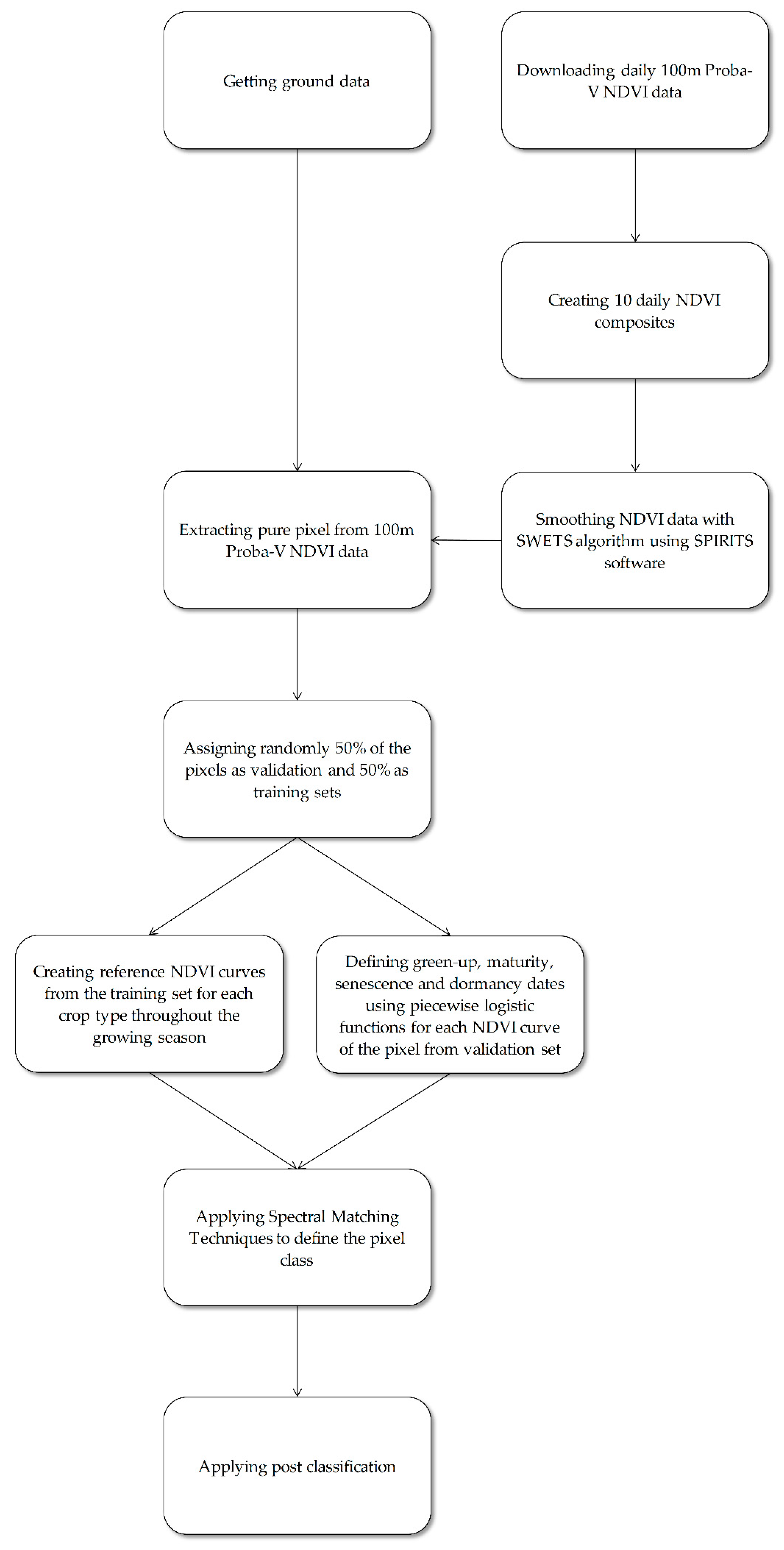
The objective of this study is to develop a crop mapping approach applicable at a global level inspired by the SMT method [21] on a seasonal basis using 100-m Proba-V NDVI data. Proba-V data at a 100-m spatial and five-day temporal resolution likely improve land monitoring studies compared to the 250-m spatial and eight-day temporal resolution of MODIS data, or the 300-m spatial and one-day temporal resolution of Proba-V, or the 10-km spatial and one-day temporal resolution of NOAA-AVHRR [25]. Although the 100-m Proba-V data tend to be more advantageous, the time series data are currently limited, as they became available in May 2013. SMTs were used for seasonal crop area mapping with time series data by using different temporal windows throughout the growing season: from green-up to senescence, from green-up to dormancy and from minimum NDVI at the beginning of the growing season to minimum NDVI at the end of the growing season. The method aims to facilitate crop production estimates by developing crop-specific maps.

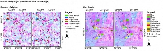
2. Materials

2.1. Study Areas and Ground Data

The study sites are globally-spread agricultural areas, which include Flanders (Belgium), Sria (Russia), Kyiv (Ukraine) and Sao Paulo (Brazil) (Figure 1). The areas are characterized by different climatic conditions, agricultural management, soil types and topography (

Table 1. Site characteristics.

Characteristics	Flanders (Belgium)	Sria (Russia)	Kyiv (Ukraine)	Sao Paulo (Brazil)
Surface Area	20,000 km2	3700 km2	11,000 km2	9000 km2
Climatic conditions	Moderate maritime climate [30]	Temperate-continental climate with cold winters and hot dry summers [31]	Humid continental [32]	Humid tropical [33]
Soil types	Albeluvisols, Luvisols, Podzols and Fluvisols [34]	Chestnut soils and chernozems [31]	Chernozems [35]	Ferralsols, 20% clay [33]
Topography	The topography is flat to hilly [36]	The topography is mostly flat with slopes ranging from 0%–2%; and nearly 15% of the territory is hilly with slopes from more than 2% [31]	The topography is mostly flat with slopes ranging from 0%–2%. Near 10% of the territory is hilly with slopes about 2%–5% [32]	The local topography is hilly, with elevations ranging from 500 m–650 m
Crop calendar	Maize: April–November [37]	Flax: April–July [31]	Winter barley: September–July [32]	Maize: September–April [37]
	Potato: March–July [37]	Maize: May–November [31]	Winter wheat: September–August [32]	Soybean: October–May [37]
	Sugar beet: April–October [37]	Peas: April–August [31]	Spring wheat: May–September [32]	Sugarcane: September–March [37]
	Winter barley: September–July [37]	Soybean: April–November [31]	Maize: May–October [32]
	Winter wheat: October–August [37]	Spring barley: April–August [31]	Rape: September–August [32]
		Sugar beet: April–October [31]	Spring barley: April–August [32]
		Sunflower: May–October [32]	Soybean: April–September [32]
		Winter barley: October–July [31]	Sugar beet: April–October [32]
		Winter rape: September–August [31]	Sunflower: May–October [32]

).

The extent and characteristics varied between the study areas (

Table 2. Crop cover characteristics of the study areas.

Study Area	Crop Type	Number of Fields	Acreage (ha)	Field Size Range (ha)	Mean Area of Fields (ha)	Ratio of Pure to Non-Pure Pixels
Flanders (Belgium)	Grain maize	42,517	36,000	1–26	1	0.01
	Potato	16,941	35,000	1–45	2	0.03
	Sugar beet	7697	19,000	1–43	2	0.04
	Winter barley	6818	11,000	1–24	2	0.02
	Winter wheat	29,910	54,000	1–37	2	0.03
Sria (Russia)	Flax	29	2098	23–298	83	1.34
	Maize	18	1755	65–167	76	1.58
	Peas	6	663	49–217	72	1.94
	Soybean	8	370	27–78	27	1.33
	Spring barley	3	165	25–82	25	1.26
	Sugar beet	1	110	110	110	1.59
	Sunflower	11	1259	49–409	73	2.15
	Winter barley	29	2276	36–172	64	1.49
	Winter rape	17	1561	53–305	91	1.72
Kyiv (Ukraine)	Winter barley	2	628	22–30	26	0.53
	Winter wheat	186	12,498	1–193	67	1.31
	Spring wheat	23	791	3–101	34	1.14
	Maize	83	4385	2–162	53	1.20
	Winter rape	49	2389	2–161	49	0.99
	Spring barley	21	628	1–143	30	0.89
	Soybean	110	3000	1–123	27	0.72
	Sugar beet	18	1623	3–270	90	1.98
	Sunflower	34	1503	3–160	44	1.20
Sao Paulo (Brazil)	Maize	30	478	2–81	16	0.39
	Soybean	91	2211	1–101	24	0.42
	Sugarcane	154	3481	1–122	23	0.41

). The number of fields of Flanders (Belgium) is relatively high compared to the other study sites, since the database covers the entire Flanders region. Sria (Russia) has the largest field sizes followed by Kyiv (Ukraine), Sao Paulo (Brazil) and Flanders (Belgium).

2.2. Ground Data

Ground data, containing crop type and parcel information, were obtained from the FP7 SIGMA (Stimulating Innovation for Global Monitoring of Agriculture) project and the digital map parcels dataset ‘GDI (Geo-Data Infrastructure)-Flanders’ [38]. The crop information in the parcels dataset was declared by farmers in Flanders-Belgium. The dataset provided a good approximation of the actual agricultural land use [39], though it cannot be regarded as 100% correct because deviations can occur due to differences in planting and declaration [40]. For Flanders (Belgium), five main crops from the parcel information database were selected: grain maize, potato, sugar beet, winter barley and winter wheat. For other study sites, the parcel size and crop type information for the 2014–2015 growing season were obtained from the SIGMA project (geoglam-sigma.info).

2.3. NDVI Data Description

Proba-V was launched in May 2013 to fill the gap between SPOT-VEGETATION and Sentinel-3 satellites. Proba-V has 4 spectral bands: blue (centered at 0.463 μm), red (0.655 μm), NIR (0.845 μm) and SWIR (1.600 μm). The central camera of the Proba-V satellite provides a 100-m data product with a 5–8 days revisiting time and daily images at 300-m and 1-km resolution. Non-composited atmospherically-corrected NDVI images from 100-m Proba-V were obtained from http://www.vito-eodata.be. Ten-daily maximum value NDVI composites were created and smoothed in SPIRITS (Software for the Processing and Interpretation of Remotely sensed Image Time Series) [41] with the algorithm of Swets et al. [42] for the growing season 2014–2015. SPIRITS is a free software used to analyze satellite-derived image time series in crop and vegetation monitoring that can be downloaded from http://spirits.jrc.ec.europa.eu/. The smoothing algorithm was used to remove higher frequency noise [43].

3. Methods

The methodology applied consisted of 5 different steps: (i) collecting training/validation samples; (ii) deriving reference NDVI profiles and phenological stages; (iii) classification using SMTs; (iv) post-classification; and (v) accuracy assessment. More details on each step is listed below, and a flowchart is presented in Figure 2:

3.1. Collecting Training/Validation Samples

For each study area, the Proba-V 100-m NDVI images were overlaid with the crop field boundaries, and both pure (i.e., homogenous pixels with a 100-m resolution) and mixed pixels were derived. In this study, only pure pixels were used. They were randomly divided into two equal groups for each crop type, one for training and one for validation. A random sampling scheme was preferred, as this is likely to prevent bias to the accuracy assessment [44].

The first Proba-V 100-m image was available during the second dekade of March 2014. The analysis was done from the first available image onwards, thereby leaving out the planting period of winter crops.

3.2. Deriving Reference NDVI Profiles and Phenological Stages

For each study area and all of the different crop types, a reference or ‘ideal’ NDVI profile was calculated by taking the average NDVI using all of the pure pixels from the training set. For Sao Paulo where double cropping occurs, the time of the year ground data were collected was taken into account to decide on the growing season. The crop calendars, which were obtained from [37,45], were used to compare with the reference NDVI profiles and establish similarity.

We used piecewise logistic functions (similar to [46]) to define the four transition dates in the reference NDVI profiles: green-up (onset of photosynthetic activity, (a) in Figure 3), maturity (maximum plant green leaf area, (b) in Figure 3), senescence (rapid decrease of photosynthetic activity and green leaf area, (c) in Figure 3) and dormancy (zero physiological activity, (d) inFigure 3) [46]. For a more detailed description of the algorithm, we refer to [46]. The four transition points defined the boundaries of different time intervals that corresponded to distinctly different crop stages. Subsequently, we compared the classification results for three time windows: from green-up to senescence ((a–c) in Figure 3), from green-up to dormancy ((a–d) in Figure 3) and from minimum NDVI at the beginning of the growing season to minimum NDVI at the end of the growing season. The different time windows were chosen to explore possibilities for early crop detection, which in turn enables crop mapping as early as possible during the growing season.

3.3. Classification Using Spectral Matching Techniques

The crop type of each pure pixel in the validation set was identified by ‘matching’ the pixel profile with different reference NDVI profiles during the specific time window within the growing periods of the reference crop type. To determine the actual crop type, the spectral similarity value (SSV) [21] was calculated between each pure pixel from the validation set and each candidate reference NDVI profile. In order to calculate SSV, the following formula was used:

$$\mathit{S}\mathit{S}\mathit{V}=\sqrt{\mathit{E}{\mathit{D}}_{\mathit{n}\mathit{o}\mathit{r}\mathit{m}\mathit{a}\mathit{l}}^{\mathbf{2}}+{\left(\mathbf{1}-\mathit{\rho }²\right)}^{\mathbf{2}}}$$

(1)

where $\rho$² and $E{D}_{normal}^2$are the correlation coefficient and the normalized Euclidean distance between the different candidate reference NDVI profiles and the pure pixel profiles, respectively. These parameters are calculated as follows:

$$\mathit{\rho }²=\frac{\mathbf{1}}{\mathit{n}-\mathbf{1}}\mathbf{\left[}\frac{{\sum }_{\mathit{i}=\mathbf{1}}^{\mathit{n}}\left(\mathit{r}\mathit{e}{\mathit{f}}_{\mathit{i}}-{\mu }_{\mathit{r}\mathit{e}\mathit{f}}\right)\left({\mathit{r}}_{\mathit{i}}-{\mu }_{\mathit{r}}\right)}{{\mathit{\sigma }}_{\mathit{r}\mathit{e}\mathit{f}}{\mathit{\sigma }}_{\mathit{r}}}\mathbf{\right]}$$

(2)

and:

$$\mathit{E}{\mathit{D}}_{\mathit{n}\mathit{o}\mathit{r}\mathit{m}\mathit{a}\mathit{l}}=\left(\mathit{E}\mathit{D}-\mathit{m}\right)/\left(\mathit{M}-\mathit{m}\right)$$

(3)

which is the normalized version of:

$$\mathit{E}\mathit{D}=\sqrt{{\sum }_{\mathit{i}=\mathbf{1}}^{\mathit{n}}{\left(\mathit{r}\mathit{e}{\mathit{f}}_{\mathit{i}}-{\mathit{r}}_{\mathit{i}}\right)}^{\mathbf{2}}}$$

(4)

where $re{f}_i$ is the reference NDVI profile at time i from 1 to n; ${\mu }_{ref}$ is the mean reference NDVI profile; $r_i$ is the pure pixel NDVI profile from validation set at time i from 1 to n; ${\mu }_{\mathrm{r}}$ is the mean pure pixel NDVI profile from validation set; ${\sigma }_{ref}$is the standard deviation of the reference NDVI profile; and ${\sigma }_r$ is the standard deviation of the pure pixel NDVI profile from the validation set. $\rho$² values vary between 0 and 1 and represent the shape of the temporal NDVI profile over time. The higher the $\rho$², the higher the similarity in the shape of the temporal NDVI profiles. The Euclidian distance (ED), normalized by using the historical minimum (m) and historical maximum (M) NDVI of the reference profile for a logical comparison, represents the closeness between the two profiles. $E{D}_{normal}$ values vary between 0 and 1. The lower the $E{D}_{normal}$, the closer the profiles are.

Accordingly, SSV is a similarity measure, which combines both the shape ($\rho$²) and distance ($E{D}_{normal}$) measures [47]. SSV values vary between 0 and a maximum of the square root of the two measures [47]. The smaller the SSV, the more similar the profiles. We assigned the pure pixel from the validation data with the label of the reference NDVI, which has the smallest SSV.

3.4. Post-Classification

In a final step, a post-classification rule was applied based on the mode value per crop type where the maximum frequency in one parcel was used to remove outliers in the classified parcel. The parcel was subsequently labelled with the crop type that had the majority of the pixels. Crop area maps were created after applying the post-classification.

3.5. Accuracy Assessment

Confusion matrices at the parcel level were constructed to compare predicted and actual class membership. Based on the confusion matrices, classification accuracy statistics included overall accuracy, producer’s accuracy, user’s accuracy and kappa coefficients. Kappa analysis provided a measure of the magnitude of agreement between the predicted and actual class membership. A kappa value of 0 represents a total random classification, while a kappa value of 1 corresponds to a perfect agreement between the reference and classification data.

4. Results

Figure 4 presents particular time windows for two selected crops in two test sites. Depending on the crop type and region, the minimum and maximum NDVI differ from each other. For instance the maximum NDVI value of soybean is close to 0.8 in Russia and 0.9 in Ukraine. Additionally, also the length of the growing season is different in different regions for the same crop, e.g., the planting and harvesting period for maize in Belgium is longer than in Brazil.

Accuracy Assessment

Overall, the proposed method using 100-m Proba V data was effective in crop type classification with relatively high accuracies. The accuracy ranged from 75%–80% in Flanders-Belgium, from 72%–86% in Sria, Russia, from 71%–86% in Kyiv, Ukraine, and from 65%–77% in Sao Paulo, Brazil (Table 3). The kappa coefficient ranged from 0.67–0.74 in Flanders-Belgium, from 0.67–0.84 in Sria, Russia, from 0.63–0.82 in Kyiv, Ukraine, and from 0.43–0.61 in Sao Paulo, Brazil (Table 3).

In all four study sites, accuracies and kappa coefficient values increased when a longer time window was considered. The results were considerably better when the time window covered the entire growing season compared to the window from green-up to senescence. Crops with similar phenological profiles were sometimes incorrectly classified particularly when only part of the growing season was considered, e.g., for summer and winter crops. When the crop growth profile had a distinctive feature compared to other crops, it was easier to differentiate it from the other crops. For instance, sugar beet in Ukraine has a longer period between maturity and senescence compared to the other summer crops. Another important outcome of the results is that post-classification improved the accuracy and kappa results for all sites, except for Belgium (see Table 3 and Table A1). The overall poorest result was obtained for producer accuracy in Brazil, due to the mixing of soybean with maize and sugarcane pixels.

Figure 5 illustrates the potential of Proba-V 100-m data for crop mapping in the study areas for selected sites. The results are shown for the pure pixels from the beginning to the end of the growing season. In general, the fields have been classified correctly for both sites. However, in Flanders (Belgium), 1 in Figure 5, some sugar beet fields have been classified as potato fields and winter wheat fields as winter barley. In Sria (Russia), 2 in Figure 5, some maize fields have been classified as sunflower and vice versa. Likewise, sunflower fields have been classified as sugar beet and winter barley as winter rape.

5. Discussion

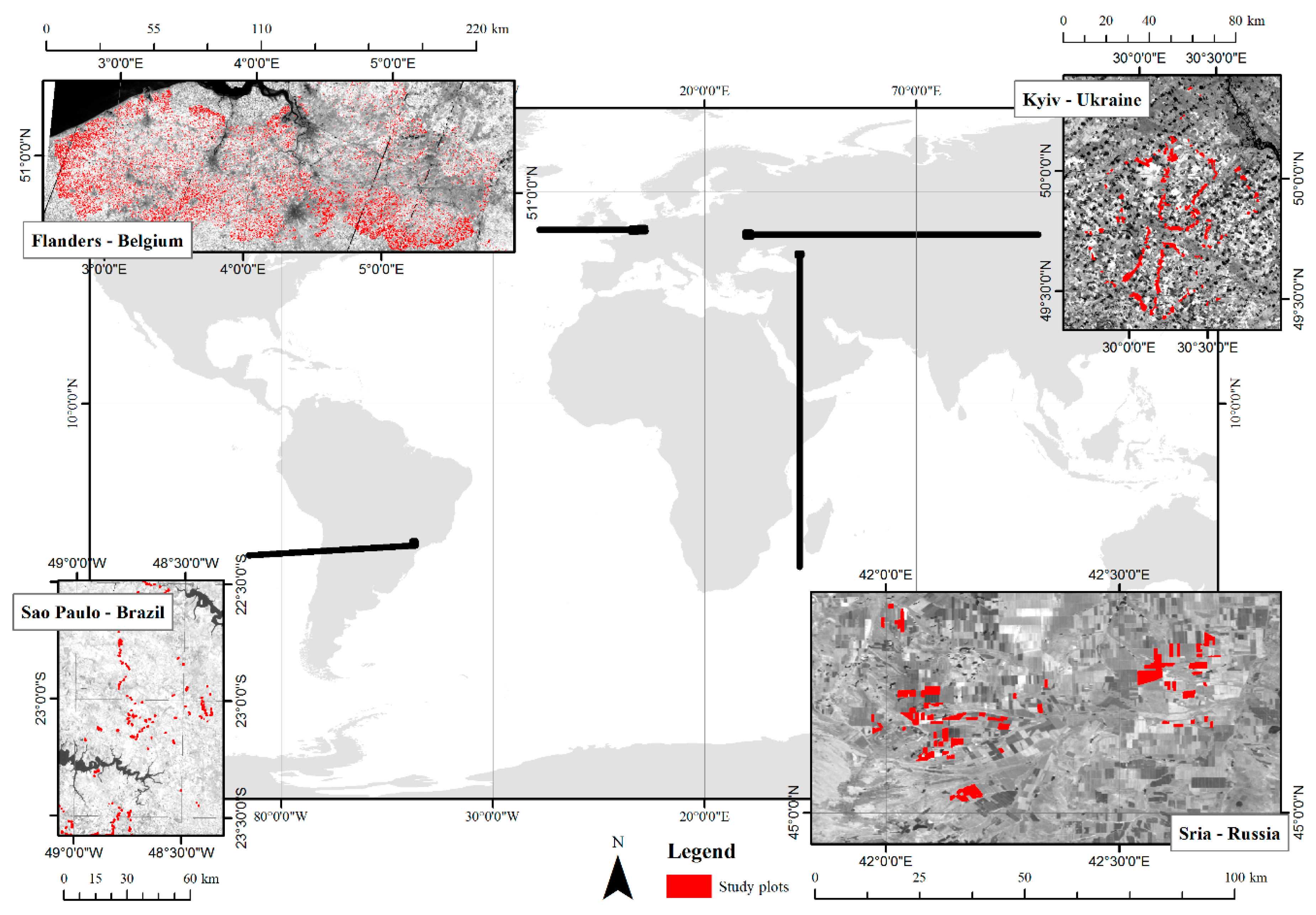
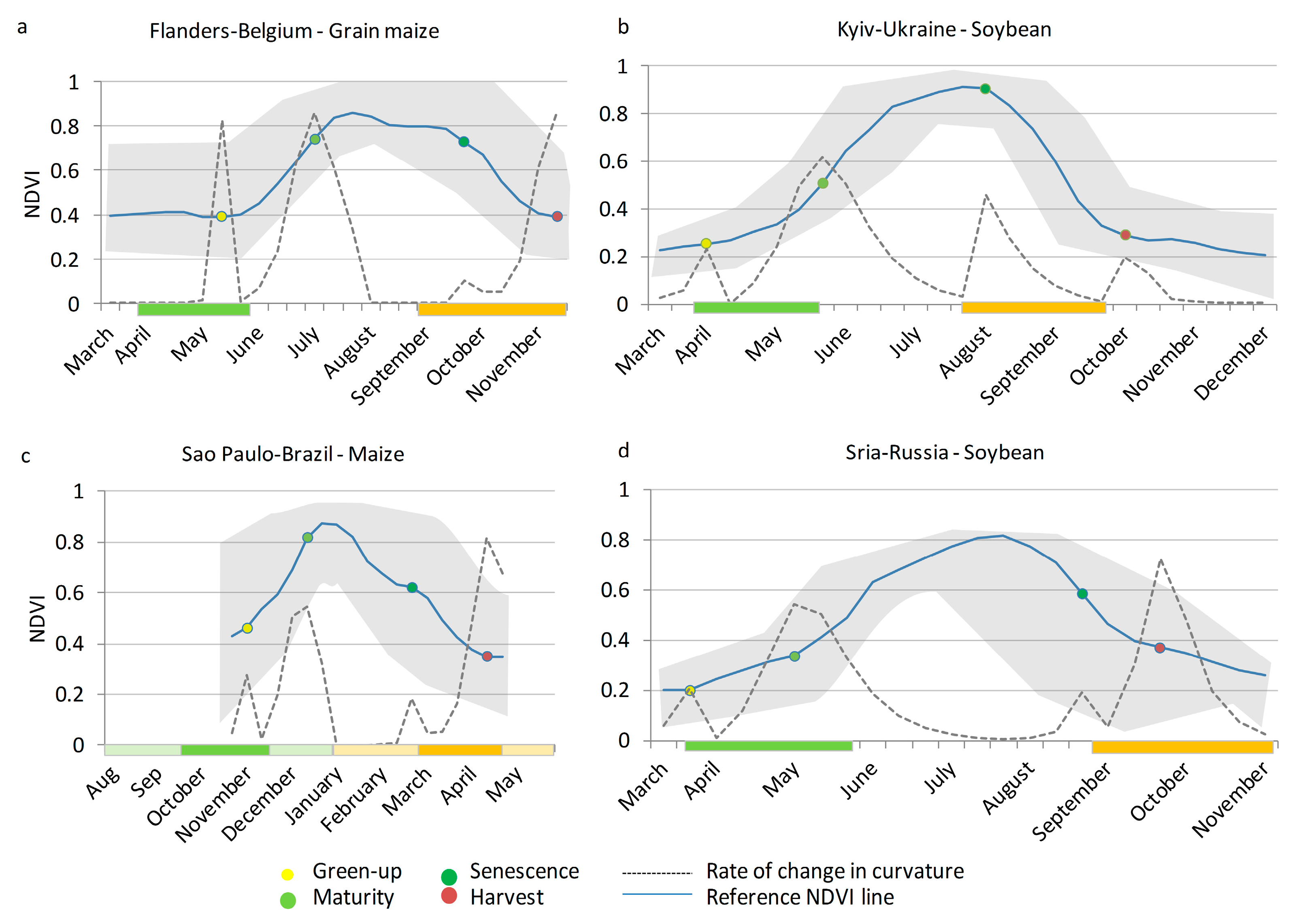
This study demonstrated the suitability of spectral matching techniques (SMTs) for mapping crop types using 100-m Proba-V data for the 2014–2015 season. The methodology integrated multi-temporal satellite imagery and parcel boundaries retrieved from both the SIGMA project and ‘GDI-Flanders’ databases. The SMTs were ideal for analyzing remote sensing time series data during the crop growth period. We calculated spectral similarity values (SSV), which are measures of the shape and magnitude similarities of the time series spectra and found the most useful SMTs, similar to [21]. Subsequently, SMTs were applied to match the ideal spectra, i.e., the reference NDVI profiles, to the class spectra, i.e., the individual pure pixel NDVI profiles.

The methodology demonstrated that 100-m Proba-V has the potential to be used in crop area mapping across different regions in the world. Proba-V is a relatively new satellite, and therefore, there are limited studies available for crop mapping. The work in [48] reported crop identification accuracies in the range of 72.4%–86.2% for 100-m Proba-V data for mapping summer and winter crops in Bulgaria. 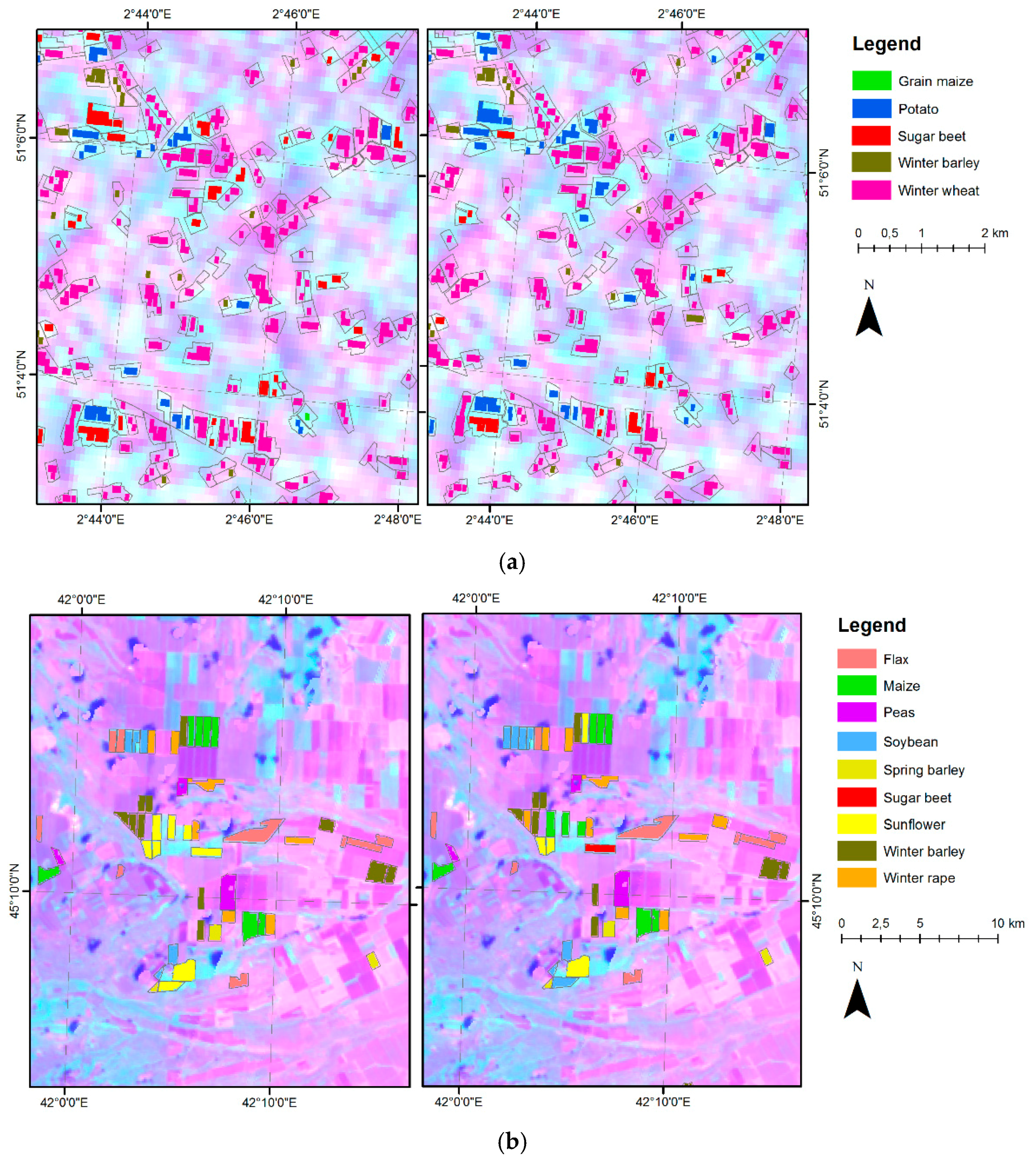In another study, [49] achieved an overall accuracy of 84% using the 100-m Proba-V sensor for cropland mapping of Sahelian and Sudanian agro-ecosystems. These reported ranges are in line with our results. When using post-classification, the overall accuracy (%) ranged between 65 and 86, and the kappa coefficient changed from 0.43–0.84. In general, post-classification improved the overall accuracy results around an additional 6%–7% for Ukraine and Brazil and 11% for Russia compared to the initial classification results. For Belgium, the post-classification technique did not improve the classification results (see Table 3 and Table A1). Our results are best in Sria, Russia, followed by Kyiv, Ukraine, Flanders-Belgium and Sao Paulo, Brazil. A couple of reasons could explain the differences between accuracies across the different study areas. Firstly, better results were observed in the areas where the crop phenological development was not spread over a long time period. For instance, the planting time for maize in Brazil stretched from August–December with a period of highest activity in October and November. This prevented extracting the distinctive characteristic of the reference NDVI profiles. Secondly, the parcel sizes played an important role. When parcels covered a small number of satellite pixels, the results were less accurate, as was the case for Belgium. Thirdly, classification errors of crop types increased when the time window covered only part of the cropping period. Another reason behind the classification errors is related to the number of ground-truth parcels available from the study site, as is the case for the winter barley fields in Kyiv, Ukraine, compared to other crop types in the same site. Finally, crops with similar growing periods might cause classification errors, such as sunflower and maize in Sria, Russia. In addition, the extent of the study area played a role. Accuracies potentially improved when region specific NDVI reference profiles were included from different agro-ecological regions. Based on these results, crop area mapping was challenging, but the use of 100_m Proba-V proved a valid option even when mapping at the field level.

Our results were in close agreement with other studies that used different classification methods and/or other higher resolution satellite images. We used a multi-temporal sequence of 100-m Proba-V images covering one to two growing seasons. The work in [8] reported an overall accuracy of 63% for vegetation mapping in southern Norway using 25-m resolution Landsat images. Another similar study reported an overall accuracy of 62.7% using the NDVI temporal profiles approach and 72.8% using a maximum likelihood classifier in the northeast of Germany with phenological information and spectral-temporal profiles from Landsat TM/ETM [16]. The use of multiple sensors seemed to increase the accuracy. For instance, [40] updated the crop classification in the land cover database of The Netherlands by combining Landsat TM, IRS-LISS3 (Indian Remote Sensing Satellite—Linear Imaging Self Scanner) and ERS2-SAR (European remote sensing satellite 2—synthetic aperture radar) and reported an overall accuracy value of 90%. Almost one million pixels were used at the national level covering not only the different types of cereals, but also grassland and flower bulbs. The use of homogeneous pixels improved the classification accuracy. The overall accuracy ranged from 73% for very heterogeneous pixels to 89% for homogeneous pixels in North Carolina and Virginia with 250-m MODIS NDVI [50]. The number of homogenous pixels used in their study was 1014, which included 475 pixels for agriculture. We presented specific crop mapping results per-field. In another study, both per-field and per-area results were presented. The work in [51] reported a maximum overall accuracy of 66% and a kappa coefficient of 0.60 per field and a maximum overall accuracy of 70% and a kappa coefficient of 0.64 per area for mapping specific crop types in Central Valley of California based on the time series of Landsat TM/ETM+.

Although our method showed promising results in crop area mapping, we identified a number of limitations. The reference NDVI profiles for the growing season of each crop type had to be defined in advance, either based on ground data, on user knowledge of the field or on a literature review. Another limiting factor occurred when the parcel size was smaller than the pixel size. Having larger parcel sizes than pixel sizes was an advantage, particularly because pure pixels tremendously improved the classification results.

The maps based on our methodology could be extended to regional or national-level crop production estimations and all crop types of interest. We showed that the within-field spectral variability could be reduced with accurate field boundaries. These boundaries eliminated classification errors due to mixed pixels [40]. Object-based image analysis could enable the detection of field boundaries in regions without parcel information. To this extent, [51] used image segmentation to delineate the field borders prior to classification.

6. Conclusions

This study demonstrated the potential of phenology-based crop type area mapping at the global level using adapted spectral matching techniques (SMTs) applied to multi-temporal 100-m Proba-V images for the 2014–2015 season. Phenological metrics were extracted from NDVI time series using piecewise logistic functions. These metrics represented the crop growing seasons and identified the unique calendar of each crop type. A distinct advantage of the SMTs was their simplicity and ease of application. In addition, the method can be extended to other areas based on the reference NDVI profiles, which are predefined either by ground data, field knowledge or literature review. The crop classification accuracies obtained could be compared favorably to the results derived from classifications with higher resolution data. The overall accuracy ranged between 65% and 86%, and the kappa coefficient varied between 0.43 and 0.84 depending on the site and the temporal window used.

References

1. Liu, M.W.; Ozdogan, M.; Zhu, X. Crop type classification by simultaneous use of satellite images of different resolutions. IEEE Trans. Geosci. Remote Sens. 2014, 52, 3637–3649. [Google Scholar] [CrossRef]
2. Reynolds, C.A.; Yitayew, M.; Slack, D.C.; Hutchinson, C.F.; Huete, A.; Petersen, M.S. Estimating crop yields and production by integrating the FAO crop specific water balance model with real-time satellite data and ground-based ancillary data. Int. J. Remote Sens. 2000, 21, 3487–3508. [Google Scholar] [CrossRef]
3. Bolton, D.K.; Friedl, M.A. Forecasting crop yield using remotely sensed vegetation indices and crop phenology metrics. Agric. For. Meteorol. 2013, 173, 74–84. [Google Scholar] [CrossRef]
4. Atzberger, C. Advances in remote sensing of agriculture: context description, existing operational monitoring systems and major information needs. Remote Sens. 2013, 5, 949–981. [Google Scholar] [CrossRef]
5. Duncan, J.M.A.; Dash, J.; Atkinson, P.M. The potential of satellite-observed crop phenology to enhance yield gap assessments in smallholder landscapes. Front. Environ. Sci. 2015, 3, 1–16. [Google Scholar] [CrossRef] [Green Version]
6. Wardlow, B.; Egbert, S.; Kastens, J. Analysis of time-series MODIS 250 m vegetation index data for crop classification in the u.s. central great plains. Remote Sens. Environ. 2007, 108, 290–310. [Google Scholar] [CrossRef]
7. Ozdogan, M.; Yang, Y.; Allez, G.; Cervantes, C. Remote Sensing of Irrigated Agriculture: Opportunities and Challenges. Remote Sens. 2010, 2, 2274–2304. [Google Scholar] [CrossRef]
8. Aurdal, L.; Ragnar Bang, H.; Eikvil, L.; Solberg, R.; Vikhamar, D.; Solberg, A. Use of hidden Markov models and phenology for multitemporal satellite image classification: Applications to mountain vegetation classification. In Proceedings of the IEEE Third International Workshop on the Analysis of Multitemporal Remote Sensing Images, Biloxi, MS, USA, 16–18 May 2005; pp. 220–224.
9. Carrão, H.; Gonçalves, P.; Caetano, M. Contribution of multispectral and multitemporal information from MODIS images to land cover classification. Remote Sens. Environ. 2008, 112, 986–997. [Google Scholar] [CrossRef]
10. Jakubauskas, M.E.; Legates, D.R.; Kastens, J.H. Crop identification using harmonic analysis oftime-series AVHRR NDVI data. Comput. Electron. Agric. 2002, 37, 127–139. [Google Scholar] [CrossRef]
11. Sakamoto, T.; Yokozawa, M.; Toritani, H.; Shibayama, M.; Ishitsuka, N.; Ohno, H. A crop phenology detection method using time-series MODIS data. Remote Sens. Environ. 2005, 96, 366–374. [Google Scholar] [CrossRef]
12. Dong, J.; Xiao, X.; Kou, W.; Qin, Y.; Zhang, G.; Li, L.; Jin, C.; Zhou, Y.; Wang, J.; Biradar, C.; et al. Tracking the dynamics of paddy rice planting area in 1986–2010 through time series Landsat images and phenology-based algorithms. Remote Sens. Environ. 2015, 160, 99–113. [Google Scholar] [CrossRef]
13. Xavier, A.C.; Rudorff, B.F.T.; Shimabukuro, Y.E.; Berka, L.M.S.; Moreira, M.A. Multi-temporal analysis of MODIS data to classify sugarcane crop. Int. J. Remote Sens. 2006, 27, 755–768. [Google Scholar] [CrossRef]
14. Alcantara, C.; Kuemmerle, T.; Prishchepov, A.V.; Radeloff, V.C. Mapping abandoned agriculture with multi-temporal MODIS satellite data. Remote Sens. Environ. 2012, 124, 334–347. [Google Scholar] [CrossRef]
15. Jönsson, P.; Eklundh, L. TIMESAT—A Program for Analyzing Time-Series of Satellite Sensor Data. Comput. Geosci. 2004, 30, 833–845. [Google Scholar] [CrossRef]
16. Foerster, S.; Kaden, K.; Foerster, M.; Itzerott, S. Crop type mapping using spectral-temporal profiles and phenological information. Comput. Electron. Agric. 2012, 89, 30–40. [Google Scholar] [CrossRef]
17. Dixon, B.; Candade, N. Multispectral landuse classification using neural networks and support vector machines: One or the other, or both? Int. J. Remote Sens. 2008, 29, 1185–1206. [Google Scholar] [CrossRef]
18. Yang, C.; Everitt, J.H.; Murden, D. Evaluating high resolution SPOT 5 satellite imagery for crop identification. Comput. Electron. Agric. 2011, 75, 347–354. [Google Scholar] [CrossRef]
19. Petitjean, F.; Inglada, J.; Gançarski, P. Satellite image time series analysis under time warping. IEEE Trans. Geosci. Remote Sens. 2012, 50, 3081–3095. [Google Scholar] [CrossRef]
20. Nitze, I.; Schulthess, U.; Asche, H. Comparison of machine learning algorithms random forest, artificial neural network and support vector machine to maximum likelihood for supervised crop type classification. In Proceedings of the 4th GEOBIA, Rio de Janeiro, Brazil, 7–9 May 2012; pp. 35–40.
21. Thenkabail, P.S.; Gangadhararao, P.; Biggs, T.W.; Krishna, M.; Turral, H. Spectral matching techniques to determine historical Land-Use/Land-Cover (LULC) and irrigated areas using time-series 0.1-Degree AVHRR pathfinder datasets. Photogramm. Eng. Remote Sens. 2007, 73, 1029–1040. [Google Scholar]
22. Gumma, M.K. Mapping rice areas of south asia using MODIS multitemporal data. J. Appl. Remote Sens. 2011, 5, 053547. [Google Scholar] [CrossRef]
23. Siachalou, S.; Mallinis, G.; Tsakiri-Strati, M. A hidden Markov models approach for crop classification: Linking crop phenology to time series of multi-sensor remote sensing data. Remote Sens. 2015, 7, 3633–3650. [Google Scholar] [CrossRef]
24. Medhavy, T.T.; Sharma, T.; Dubey, R.P.; Hooda, R.S.; Mothikumar, K.E.; Yadav, M.; Manchanda, M.L.; Ruhal, D.S.; Khera, A.P.; Jarwal, S.D. Crop classification accuracy as influenced by training strategy, data transformation and spatial resolution of data. J. Indian Soc. Remote Sens. 1993, 21, 21–28. [Google Scholar] [CrossRef]
25. Dadhwal, V.K.; Ruhal, D.S.; Medhavy, T.T.; Jarwal, S.D.; Khera, A.P.; Singh, J.; Sharma, T.; Parihar, J.S. Wheat acreage estimation for Haryana using satellite digital data. J. Indian Soc. Remote Sens. 1991, 19, 1–15. [Google Scholar] [CrossRef]
26. Chmielewski, F.-M.; Müller, A.; Bruns, E. Climate changes and trends in phenology of fruit trees and field crops in Germany, 1961–2000. Agric. For. Meteorol. 2004, 121, 69–78. [Google Scholar] [CrossRef]
27. Van Niel, T.G.; McVicar, T.R.; Fang, H.; Liang, S. Calculating environmental moisture for per-field discrimination of rice crops. Int. J. Remote Sens. 2003, 24, 885–890. [Google Scholar] [CrossRef]
28. Wardlow, B.D.; Egbert, S.L. Large-Area Crop Mapping using time-series MODIS 250 m NDVI data: An assessment for the U.S. central great plains. Remote Sens. Environ. 2008, 112, 1096–1116. [Google Scholar] [CrossRef]
29. Lu, D.; Weng, Q. A survey of image classification methods and techniques for improving classification performance. Int. J. Remote Sens. 2007, 28, 823–870. [Google Scholar] [CrossRef]
30. Cools, M.; Moons, E.; Creemers, L.; Wets, G. Changes in Travel Behavior in Response to Weather Conditions. In Proceedings of the CD 89th Annual Meeting of the Transportation Research Board, Washington, DC, USA, 10–14 January 2010.
31. JECAM. Russia—Stavropol Kray. Available online: http://www.jecam.org/?/site-description/russia-stavropol-kray (accessed on 14 June 2016).
32. JECAM. Ukraine—Kyiv. Available online: http://www.jecam.org/?/site-description/ukraine (accessed on 14 June 2016).
33. JECAM. Brazil—São Paulo. Available online: http://www.jecam.org/?/site-description/Brazil-Sao-Paulo-Itatinga (accessed on 14 June 2016).
34. Peeters, A. Country Pasture/Forage Resource Profile for Belgium. Available online: http://www.fao.org/ag/AGP/AGPC/doc/Counprof/Belgium/belgium.htm (accessed on 14 June 2016).
35. Słowińska-Jurkiewicz, A.; Bryk, M.; Medvedev, V.V. Long-Term organic fertilization effect on chernozem structure. Int. Agrophys. 2013, 27, 81–87. [Google Scholar]
36. JECAM. Belgium. Available online: http://www.jecam.org/?/site-description/belgium (accessed on 14 June 2016).
37. AMIS. AMIS Crop Calendar; AMIS: Rome, Italy, 2012. [Google Scholar]
38. AGIV. GDI-Vlaanderen Landbouwgebruikspercelen ALV, 2014. Available online: http://www.geopunt.be/download?container=landbouwgebruikspercelen&title=Landbouwgebruikspercelen 2014 (accessed on 24 February 2016).
39. Verhoeve, A.; Dewaelheyns, V.; Kerselaers, E.; Rogge, E.; Gulinck, H. Virtual farmland: Grasping the occupation of agricultural land by non-agricultural land uses. Land Use Policy 2015, 42, 547–556. [Google Scholar] [CrossRef]
40. De Wit, A.J.W.; Clevers, J.G.P.W. Efficiency and accuracy of per-field classification for operational crop mapping. Int. J. Remote Sens. 2004, 25, 4091–4112. [Google Scholar] [CrossRef]
41. Rembold, F.; Meroni, M.; Urbano, F.; Royer, A.; Atzberger, C.; Lemoine, G.; Eerens, H.; Haesen, D.; Aidco, D.G.; Klisch, A. Remote sensing time series analysis for crop monitoring with the SPIRITS software: New functionalities and use examples. Front. Environ. Sci. 2015, 3, 129–134. [Google Scholar] [CrossRef]
42. Swets, D.; Reed, B.; Rowland, J.; Marko, S. A Weighted Least-Squares Approach to Temporal NDVI Smoothing. In Proceedings of the 1999 ASPRS Annual Conference from Image to Information, Portland, OR, USA, 17–21 May 1999.
43. Geerken, R.A. An algorithm to classify and monitor seasonal variations in vegetation phenologies and their inter-annual change. ISPRS J. Photogramm. Remote Sens. 2009, 64, 422–431. [Google Scholar] [CrossRef]
44. Yu, Q.; Gong, P.; Tian, Y.Q.; Pu, R.; Yang, J. Factors affecting spatial variation of classification uncertainty in an image object-based vegetation mapping. Photogramm. Eng. Remote Sens. 2008, 74, 1007–1018. [Google Scholar] [CrossRef]
45. Homayouni, S.; Roux, M. Hyperspectral image analysis for material mapping using spectral matching. Int. Arch. Photogramm. Remote Sens. Spat. Inf. Sci. 2004, 35, 1682–1750. [Google Scholar]
46. Zhang, X.; Friedl, M.A.; Schaaf, C.B.; Strahler, A.H.; Hodges, J.C.F.; Gao, F.; Reed, B.C.; Huete, A. Monitoring vegetation phenology using MODIS. Remote Sens. Environ. 2003, 84, 471–475. [Google Scholar] [CrossRef]
47. Cheema, M.J.M.; Bastiaanssen, W.G.M. Land use and land cover classification in the irrigated Indus Basin using growth phenology information from satellite data to support water management analysis. Agric. Water Manag. 2010, 97, 1541–1552. [Google Scholar] [CrossRef]
48. Roumenina, E.; Atzberger, C.; Vassilev, V.; Dimitrov, P.; Kamenova, I.; Banov, M.; Filchev, L.; Jelev, G. Single- and multi-date crop identification using Proba-V 100 and 300 m S1 products on Zlatia Test Site, Bulgaria. Remote Sens. 2015, 7, 13843–13862. [Google Scholar] [CrossRef]
49. Lambert, M.; Waldner, F.; Defourny, P. Cropland mapping over sahelian and sudanian agrosystems: A knowledge-based approach using Proba-V time series at 100-m. Remote Sens. 2016, 8, 232. [Google Scholar] [CrossRef]
50. Knight, J.F.; Lunetta, R.S.; Ediriwickrema, J.; Khorram, S. Regional scale land cover characterization using MODIS-NDVI 250 m multi-temporal imagery: A phenology-based approach. GISci. Remote Sens. 2007, 43, 1–23. [Google Scholar] [CrossRef]
51. Zhong, L.; Gong, P.; Biging, G.S. Phenology-Based crop classification algorithm and its implications on agricultural water use assessments in California’s Central Valley. Photogramm. Eng. Remote Sens. 2012, 78, 799–813. [Google Scholar] [CrossRef]
Figure 1. Study sites overlaid with field boundaries. The background images were extracted from the100-m Proba-V red band.
Remotesensing 08 00585 g001
Figure 2. Flowchart of the crop mapping methodology.
Remotesensing 08 00585 g002
Figure 3. A schematic presentation of the annual cycle of crop phenology characterized by four key transition dates ((a) green-up; (b) maturity; (c) senescence and (d) dormancy) calculated using values in the rate of change in the curvature (adapted from [46]).
Remotesensing 08 00585 g003
Figure 4. (ad) Crop time windows for maize in Flanders-Belgium (a) and Sao Paulo, Brazil (c); and for soybean in Kyiv, Ukraine (b), and Sria, Russia (d). The four phenological transition dates were calculated from piecewise logistic functions. The grey zone represents the minimum and maximum NDVI values in the training dataset. The crop calendar for each study site is presented below each graph, where green represents the planting time and orange the harvesting time. Light green and orange colors represent periods with low activity for maize in Brazil.
Remotesensing 08 00585 g004
Figure 5. Comparison of the classification results based on pure pixels during the entire growing season for a selected area in Flanders-Belgium (a) and Sria, Russia (b). (Left) The overlay of Proba-V and ground/field data; (right) the overlay with the post-classification results.
Remotesensing 08 00585 g005