Article

Analysis and Mapping of the Spectral Characteristics of Fractional Green Cover in Saline Wetlands (NE Spain) Using Field and Remote Sensing Data

by
Manuela Domínguez-Beisiegel
1,
Carmen Castañeda
2,*,
Bernard Mougenot
3 and
Juan Herrero
2
1
Agrifood Research & Technology Center of Aragon (CITA), EEAD-CSIC Associated Unit, Ave. Montañana 930, 50059 Zaragoza, Spain
2
Estación Experimental de Aula Dei, EEAD-CSIC, Ave. Montañana 1005, 50059 Zaragoza, Spain
3
Centre d’Etudes Spatiales de la Biosphère, (CESBIO), Université de Toulouse, CNES/CNRS/IRD/UPS, 18 Av. Eduard Belin, 31401 CEDEX 9 Toulouse, France
*
Author to whom correspondence should be addressed.
Submission received: 29 February 2016 / Revised: 13 June 2016 / Accepted: 7 July 2016 / Published: 13 July 2016
(This article belongs to the Special Issue What can Remote Sensing Do for the Conservation of Wetlands?)

Abstract

:
Inland saline wetlands are complex systems undergoing continuous changes in moisture and salinity and are especially vulnerable to human pressures. Remote sensing is helpful to identify vegetation change in semi-arid wetlands and to assess wetland degradation. Remote sensing-based monitoring requires identification of the spectral characteristics of soils and vegetation and their correspondence with the vegetation cover and soil conditions. We studied the spectral characteristics of soils and vegetation of saline wetlands in Monegros, NE Spain, through field and satellite images. Radiometric and complementary field measurements in two field surveys in 2007 and 2008 were collected in selected sites deemed as representative of different soil moisture, soil color, type of vegetation, and density. Despite the high local variability, we identified good relationships between field spectral data and Quickbird images. A methodology was established for mapping the fraction of vegetation cover in Monegros and other semi-arid areas. Estimating vegetation cover in arid wetlands is conditioned by the soil background and by the occurrence of dry and senescent vegetation accompanying the green component of perennial salt-tolerant plants. Normalized Difference Vegetation Index (NDVI) was appropriate to map the distribution of the vegetation cover if the green and yellow-green parts of the plants are considered.

Graphical Abstract

1. Introduction

A goal of the European Habitats Directive is to protect biodiversity through the conservation of habitats (Council Directive 92/43/EEC). The Directive establishes the designation of protected areas to be included in the Natura 2000 network. The implementation of this network requires the monitoring and management of habitats and stresses the urgent need for updated information on habitat conservation status. Remote sensing can provide useful data for mapping and monitoring protected habitats [1,2,3,4,5] and assessing vegetation cover at detailed scales using aerial ortho-images, or high resolution airborne or satellite imagery such as Quickbird, Ikonos [6,7,8,9,10], or the most recent Worldview and Geo-Eye satellites [11,12,13,14], and to establish a relationship between vegetation cover, type or biological crust, and its phenological state using satellite data [15,16].
Habitat preservation requires continued monitoring [3] the distribution of habitats and their conservation status. Vegetation changes have been estimated in arid areas using Landsat images [17,18,19,20]. A large number of studies quantify vegetation cover using vegetation indices based upon Landsat images and field surveys [7,17,21,22]. Quickbird images are suitable for plant cover estimation and vegetation mapping in semi-arid areas, given their high spatial resolution [23]. However, the spectral range (445–900 nm) limits the study of plant cover [24] to chlorophyll and leaf structure effects, and less to leaf moisture effects which can be directly sensed in the SWIR. Notwithstanding, Duchemin [25] showed that the improvement of spatial resolution of Quickbird images, compared with Landsat images, results in a better relationship between satellite and field spectral data in heterogeneous areas.
The fraction of green cover has been estimated through satellite imagery, aerial photography, or directly from field data using different techniques [23,26]. Laliberte et al. [27] combined image segmentation and object-based classification of aerial photographs and Quickbird images to quantify changes of vegetation cover in New Mexico. Laliberte et al. [23] obtained an underestimation of total and senescent vegetation by 5% using digital ground photographs and object-based classification of Quickbird images in arid regions of the southwestern US. Spectral unmixing techniques have been applied in a variety of environments and scales, using fine and coarse resolution imagery such as Landsat to estimate sub pixel proportions of ground components [13,28,29,30,31,32,33].
Vegetation in arid environments is characterized by open canopies with significant background (leaf litter, dead branches, shadows, and soil) making it difficult to isolate the green vegetation reflectance signal from the canopy background signal [34]. Mapping and estimating vegetation cover in arid areas at detailed scales is hindered by the sparsity of vegetation and the influence of soil background reflectance in the spectral data [15,17,35,36,37,38,39]. Moreover, green vegetation cover can be overestimated if the Normalized Difference Vegetation Index (NDVI) is used for sparse vegetation due to the high reflectivity of bright soils and the abundance of non-photosynthetic vegetation [7]. As Montandon and Small [40] pointed out, the assumption that NDVI of bare soil is 0, results in overestimation of NDVI and vegetation quantity, especially in areas with sparse vegetation cover. Todd and Hoffer [39] showed that for vegetation covers between 20% and 80%, NDVI values were higher for moist soils than for dry soils, and that soil moisture influences more the reflectance of vegetation than soil type.
Glenn et al. [41] established the relationship between NDVI extracted from high-resolution aerial images (pixel of 0.3 m) and the fraction of green vegetation of plants with leaves of different shapes and angle throughout the growing season. Maas [42] studied the effect of the spectroradiometer point of view on the reflectance of vegetation in the field, observing a decrease of reflectance as shadows between plants increased. Some studies try to establish quantitative and qualitative relationships between spectral data and vegetation cover [11] and the characteristics of soils with biological crust [16,43,44,45].
The development stage of vegetation in saline wetlands is subjected to water and salt stresses resulting in a complex and highly variable environment [46] with sudden unpredictable changes. There is no a standard methodology to examine the temporal changes of such environments. European Directives and national rules enforce the conservation and protection of priority habitats. A methodology is needed to overcome the lack of regular ground data in RAMSAR sites such as the Monegros saline wetlands [47], in order to face their destruction due to the agricultural intensification, especially new irrigation schemes. Satellite images are a major data source for habitat monitoring, capturing information on the condition of protected areas and their surroundings, and the changes in habitat extent and spatial patterns. The fraction of green cover is a sensitive indicator of land degradation [7] and can be used to study changes in vegetation in arid areas.
The objective of our work was to develop an integrated methodology for monitoring the vegetation of saline wetlands using remote sensing. For this purpose, we first analyzed the spectral characteristics of soils and vegetation in Monegros saline wetlands during the 2007 and 2008 field campaigns using field spectra and synchronous soil and vegetation data. Secondly, we established a relationship between the fraction of green cover and the spectral data from Quickbird images. Thirdly, the NDVI values calculated from Quickbird images were compared to NDVI values calculated from Landsat ETM+ and ASTER images to find out if these data could be applied for mapping the fraction of vegetation cover.

2. Study Area

The Monegros desert, NE Spain, (Figure 1) hosts around 149 saline wetlands, locally named “saladas”, with a total area extent of 1917 ha [48]. The saladas are spread in an agricultural landscape, and are very close to irrigated lands, at elevation between 320 and 417 m above sea level. The area is one of the most arid regions in Europe [49], with 346 mm of mean annual precipitation for the Bujaraloz-Petris weather station situated at 345 m above sea level (41.43°N–0.15°E). Rainfall is very irregular, ranging annually between 175 mm and 535 mm. The mean annual evapotranspiration ET0 is 1255 mm based on the estimate of [50] for the nearby Bujaraloz weather station.
For the period of this study, the cumulative rainfall from January to the end of June was 171 mm, in 2007, similar to the long term mean for the same period, and 273 mm, in 2008, being 63% higher than in 2007. The minimum temperature was −10.2 °C in January 2007 and the maximum was 38.3 °C in August 2007.
From the 149 inventoried saline wetlands, 114 have natural vegetation that covers 38% of the total area. Halophytes (plants growing in a soil with a high content of salts) occur in 90 wetlands, the rest are partially or totally cultivated [48,51]. The Monegros saline wetlands host a high biodiversity, each wetland includes between two and 17 CORINE habitats and between two and seven habitats of Community interest under the Habitats Directive 92/43/EEC. Part of the habitats has been already destroyed due to the disappearance or the degradation of these wetlands [51,52]. Vegetation typically fringes the bare hypersaline floors of the playa-lakes or covers the bottom of saline depressions, conditioned by soil microtopography, moisture, and salinity. Due to the intermittent flooding, the soil surface is prone to frequent changes in soil moisture and salinity, and to variable occurrence of efflorescences (whitish fluffy or crystalline powder surface encrustation on a soil produced by evaporation of water brought to the surface by capillarity or by loss of water on exposure to the air [53]) and salt crusts. Soil texture at the saladas bottom is silty or silty clay [54].
Xero-halophilous (salt-tolerant shrub formations of dry ground in low-precipitation areas [55]) scrubs (Arthrocnemum macrostachyum, Suaeda vera subsp. braun-blanquetii, Limonium latebracteatum) and Lygeum spartum, predominate in saline soils and occupy high topographic positions. Annual plants (Frankenia pulverulenta, Sphenopus divaricatus, Halopeplis amplexicaulis, Salicornia patula, Microcnemum coralloides) frequently pioneer the playa-lake floor. Xero-halophilous and halo-nitrophilous (plants preferring or thriving in a saline soil [55]) scrubs and grasses are interspersed with meadows of halophilous therophytes (annual plants which survive adverse season through their seed [56]) or tamarisk (Tamarix canariensis) communities [48].

3. Material and Methods

Figure 2 summarizes the methodology followed to integrate field and satellite data. Two field campaigns were conducted during the summers of 2007 and 2008, based on a georeferenced database of vegetation [48,57]. Surveys were done in summer, when perennial halophytes reach maximum photosynthetic activity. Field radiometry campaigns were synchronized with satellite images.

3.1. Sampling Sites and Instruments

A total of 11 wetlands were sampled, nine in 2007 and six in 2008 (Figure 1); four of them were surveyed in both years. Their size ranges from 134 ha to 240 ha. A. macrostachyum and S. vera were the most representative plants from the point of view of the surface extent (162 ha) together with the bare soil (342 ha). We sampled points deemed as representative of the covers to be discriminated by remote sensing, i.e., bare soils intermittently flooded with different moisture and surface conditions (salt crust, efflorescence), and vegetation with representative plants and different percent cover.
A CropScan MSR16R multispectral radiometer (16 bands centered between 450 nm and 1750 nm with bandwidth ≅ 10 nm) was used in 2007 to record the reflectivity of samples of soil or vegetation in a total of 144 locations, 4–34 points at each wetland. A continuous spectrum (2020 bands between 200 and 1100 nm, with spectral resolution from 0.035 to 6.8 nm) was recorded in 2008, using the Ocean Optics HR2000CG-UV-NIR spectrometer along 17 transects 24 to 150 m long. There were from two to five transects in each wetland, and each transect included from four to nine points, 90 sampling points. The readings were collected from 11:00 to 15:00 and calibrated with a 50% (grey) SpectralonTM reflectance standard panel (Labsphere, Inc., North Sutton, NH, USA). Sample and panel readings were corrected by subtracting the dark spectrum of the instrument. Then, the reflectance values were calculated as 0.5 × sample value/panel value, where 0.5 is the correction factor of the grey panel. Five spectral measurements per point were averaged and filtered.
The reflectance of samples in four CropScan channels (485, 561, 660, and 830 nm) was directly compared with that of the corresponding Quickbird bands, with centers and bandwidths of 488 nm (430–545), 542 nm (466–620), 650 nm (590–710), and 817 nm (715–918). The raw data from Ocean Optics were pre-processed using SAMS (Spectral Analysis Management System) software originally developed at the University of California Davis Center for Spatial Technologies and Remote Sensing (CSTARS). The pre-processed continuum spectra, exported to the ENVI® spectral library, were sampled into the Quickbird discrete bands using the Spectral Library Resampling tool. We sampled the band 4 (NIR) within the range 775–795 nm to eliminate noisy absorption values. NDVI [(NIR − VIS)/(NIR + VIS)] was calculated from the field spectra (NDVIField).

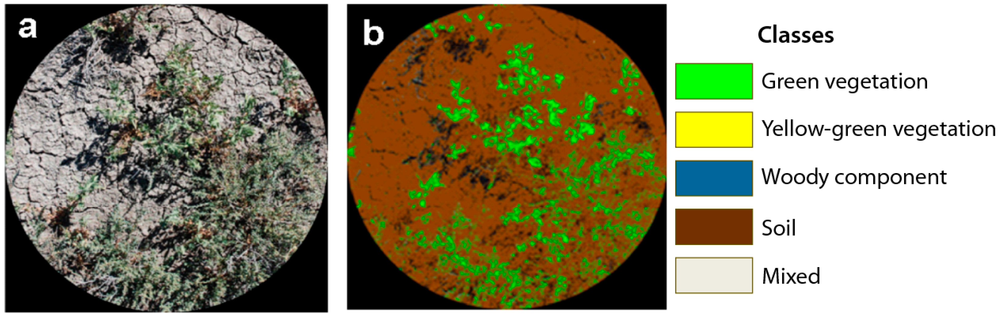
3.2. Ground Photography and Auxiliary Field Data

A vertical photograph (18 mm camera lens) of the ground was taken on a tripod at 1.3 m height with a similar nadir to the spectrometer in 2008, simultaneous with each spectral measurement (Figure 2). The photographs, covering 167 cm × 111 cm on the ground, were classified with Can-Eye software [58] by supervised classification to obtain the fraction of vegetation cover (fCover) [59]. The reflectance of control samples with four different percent covers of vegetation (0%, 25%, 50%, and 100%) prepared by visual comparison with Munsell standards was recorded. At each sampling point we took a visual estimation of plant cover, the Munsell soil color hues, and the gravimetric soil moisture of the two first centimeters of soil. For this purpose we determined the difference in weight after drying the soil samples at 40 °C according to [60].

3.3. Satellite Images and Data Processing

Two Quickbird images were acquired in summer (July 2007 and 2008) scheduled in correspondence with the field campaigns. Due to the 16.5 km-limited Quickbird width-imaging swath, three sub-images were acquired between two dates (spanning 18 days) to complete the entire study area in July 2007. A single Quickbird image was acquired for 2008 survey, adapted to the surveyed area.
We checked the radiometric homogeneity of the field sites on the georeferenced Quickbird image and we selected only the most homogeneous points with vegetation or bare soil, i.e., the pure points. The fCover, estimated from the ground photographs, was related to NDVI from field spectra (NDVIField) which was related to the NDVI calculated from the Quickbird image (NDVIQB) (Figure 2).
Furthermore, the effects of spatial and spectral resolution on the identification of the studied vegetation were analyzed by comparing Landsat and ASTER summer images with Quickbird and field spectral data. Landsat and ASTER images were processed similar to QB images. The dry summer of 2007, with absence of rains before the capture of these images, guaranteed similar soil surface conditions for all data sources. The characteristics of the satellite images are summarized in Table 1.
Satellite image processing included radiometric, atmospheric, and geometric corrections. Radiometric corrections and conversion of image brightness to Top of Atmosphere (TOA) reflectance were made using ACORN5 software (ImSpec, Palmdale, CA, USA) based on the MODTRAN4 (MODerate resolution atmospheric TRANsmission) algorithm. The geometric correction was applied using more than 20 ground control points (GCP) and orthophotographs from 2006 supplied by the Spanish Geographical Institute (IGN) with 0.5 m pixel size. A second order polynomial equation and the nearest neighbor resampling were used to rectify the images, yielding root mean square errors <0.5 pixel in all cases. We masked the image values outside of the wetlands using the wetlands inventory boundary [51].
The resulting fCover map was classified using a decision tree classifier of ENVI® with fCover and NDVIField images as input data. For NDVIField values <0, two soil moisture classes were established: <20% and ≥20%, after the soil moisture recorded in the field. For NDVIField values >0, classes of fCover were established at 10% increments.

4. Results

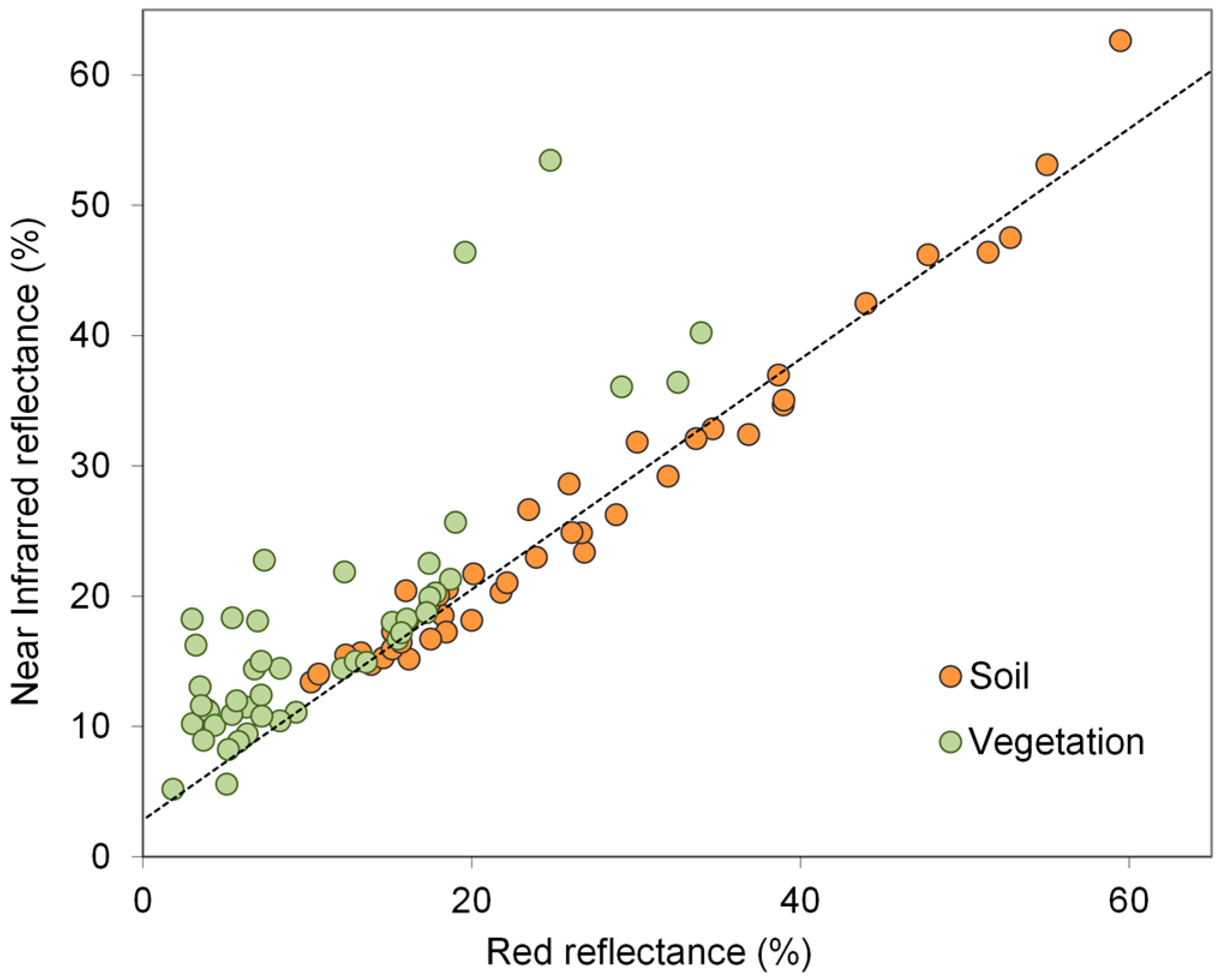
4.1. Spectral Characteristics of Soil and Vegetation

Data of sampling points with spectrometer Ocean Optics are summarized in Table S1. Mean soil reflectance ranges from 30% to 40% in the visible (VIS) and near infrared (NIR) spectra, respectively, and reaches 50% in soils with efflorescence (Figure 3). Dry soils without efflorescence show continuously increasing reflectance from the VIS to NIR. The soil surface frequently exhibited light colors, with Munsell values of 7 and 8, due to the soil composition. Gypsum and carbonates are ubiquitous in the landscape due to the parent material; the 0–15 cm soil layer is characterized by 10% to 91% of gypsum and 12% to 45% of calcium carbonate [61].
The occurrence of efflorescence increases the reflectivity of moist or saturated soils (Figure 3). Sapropelic layers (limnic fetid slime or strongly reduced soil [62]) cause a general decrease of the reflectance, showing by about 8% along the VIS and NIR excepting if efflorescence occurs (Figure 3).
Dark soils have Munsell values of 4 or less and a reflectance ranging from 10% to 20%. In spite of the scarce rains, high evaporation, and desiccating winds during the dry season, the soil remained moist at the saladas floor, with a gravimetric moisture content ranging from 0.4% to 24% in the top two centimeters of soil. Moist soils show half the reflectance of dry soils: 10% to 20% in the VIS and 20% to 25% in the NIR spectra (Figure 4).
The spectral measures of control samples, arranged with different percent cover of vegetation by visual comparison with Munsell standards (25%, 50%, and 100%), show a similar shape (Figure 4). The reflectance decreases with the increase of vegetation cover and soil moisture. In general, visible reflectance is about 20% less and near-infrared reflectance is 20%–30% higher. The difference between the reflectance of dry and moist soils decreases as the percent cover of vegetation increases. The maximum difference is about 10% and remains constant along the whole VIS-NIR spectra in areas with ≤25% cover of vegetation.
Field spectra of different plants with about 100% percent cover (Figure 5) give a similar spectral signature with a relative low spectral signal. In general VIS reflectance is lower than 5% and NIR reflectance <30%. Hyper-halophilous plants such as Salicornia ramosissima, pioneering the bare soil (Figure 5a), present the highest and most variable reflectance, reaching up to 35% due to the contribution of the soil background (Figure 5a). Halophytes show a 20% difference between VIS and NIR reflectance and a slight peak of reflectance in the green part of spectra. Juncus maritimus exhibits the lowest reflectance (VIS reflectance <5%) due to the reflectance from dry parts of the plant (Figure 5b). Despite the differences in plant color and morphology, Lygeum spartum (Figure 5c), Microcnemum coralloides (Figure 5d), and Salsola kali (Figure 5e) have similar spectral responses. Suaeda vera (Figure 5f) presents one of the highest differences between VIS and NIR (10%) even although this plant had a high proportion of senescent component during the dates of the study, and because of that the maximum near-infrared reflectance is below 25%. As the proportion of the green component increases in the plant, the difference between VIS and NIR spectra increases.

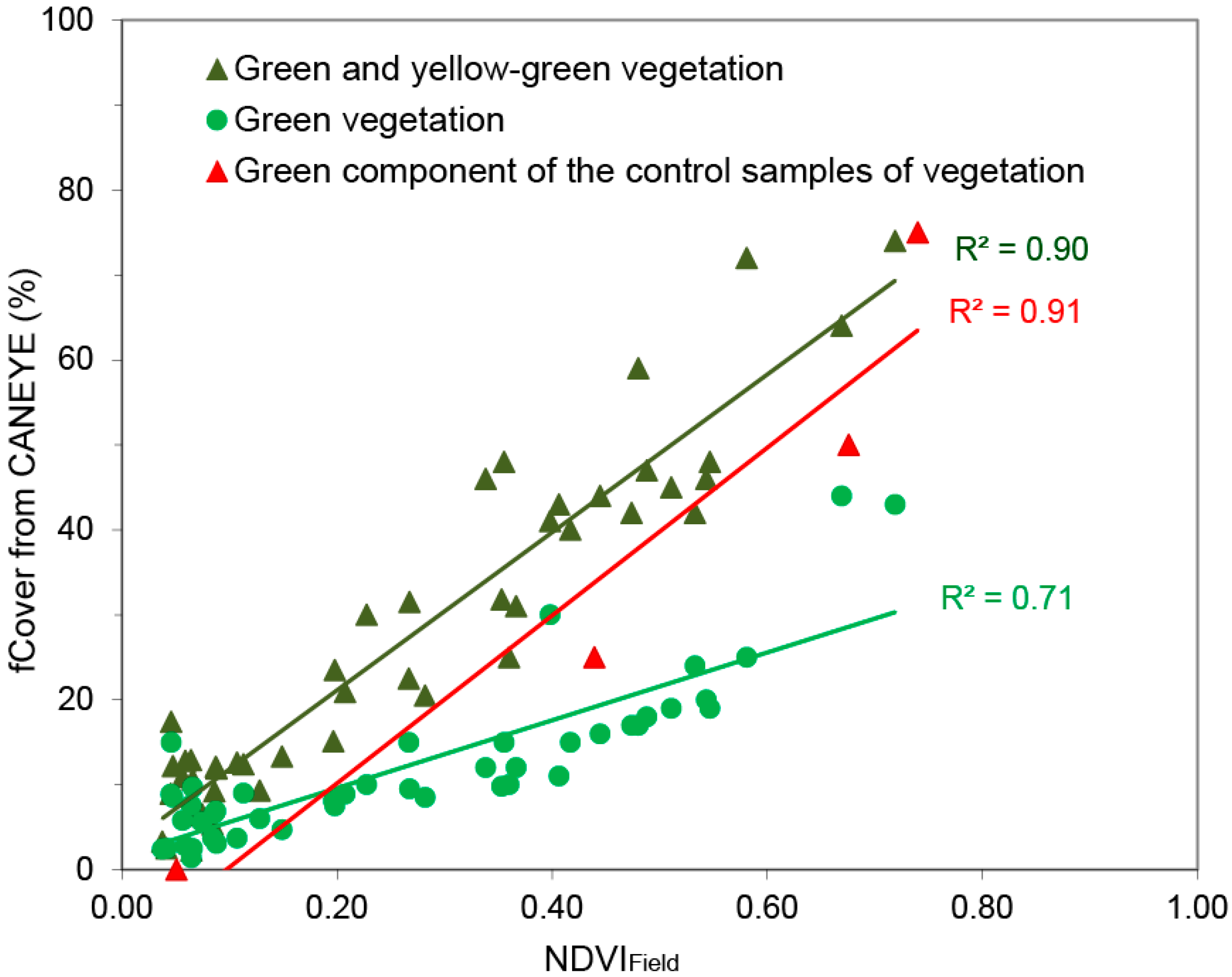
4.2. NDVI and Green Cover Fraction

Five classes resulted from the classification of field photographs (Figure 6): green and yellow-green vegetation, woody component, bare soil, and mixed areas corresponding to shadows and pixels not included in the previous classes. The fraction of green vegetation extracted from the field photographs varies from 1.4% to 44%, with 22% as the mean. The yellow-green fraction of vegetation includes senescent vegetation, and is largely represented in our sampling points. Very yellow vegetation was not included because it was not chlorophyllic and did not contribute to the NDVI but to the bare soil spectra. If we total green plus yellow-green (or senescent) vegetation, the fCover increases to an average of 27%, ranging from 2.3% to 74%.
Dark colored soils (chroma ≤4) have from 2% to 18% of soil moisture whereas light colored soils (chroma >5) are usually completely dry. The percentage of the five classes differs depending on the soils chroma. On average, green and yellow-green fractions of vegetation are higher in dark soils whereas the percentage of woody component increases in light colored soils (Table 2).
The relationship between the percentage of vegetation extracted from vertical photographs (fCover) and NDVI derived from simultaneous readings of spectra depends on the vegetation classes considered (Figure 7). A good relationship with a coefficient of determination R2 = 91% was obtained by taking into account the green component of control samples. As shown in Figure 7, a 100% of vegetation cover in the field results in 75% of fCover from the classification of the vertical photograph. This result is comparable with that obtained for sampled points if green and yellow-green fractions are included in the total amount of vegetation, R2 = 90% (RMSE = 6.09%). However, R2 decreases to 71% (RMSE = 5.07%) if only the green fraction is considered (Figure 7).
The spectrometer measures overestimate NDVI of control samples at 50% of vegetation cover due to the contribution of the soil background with a high reflectance in NIR, and underestimate the NDVI of 100% vegetation cover areas due to the shadows contribution. On the other hand, fCover underestimates the vegetation cover if compared to visual appraisal, even if fCover is computed as the green plus the yellow-green fractions. It is due to the effect of shadows and the difficulty of classifying the wide range of green and yellow­green hues occurring in the photographs.
Assuming an arbitrary NDVI value of 0.2 to separate soil and vegetation our sampling shows that 40% of the vegetation should be considered bare soil. The soil line, i.e., the line where the bare soil reflectance concentrates [63], also includes the sampling points characterized by sparse vegetation with dark green color (Figure 8). This Figure resembles the classic Tasselled Cap shape, although with few samples high in NIR and low in red since it is an arid environment.

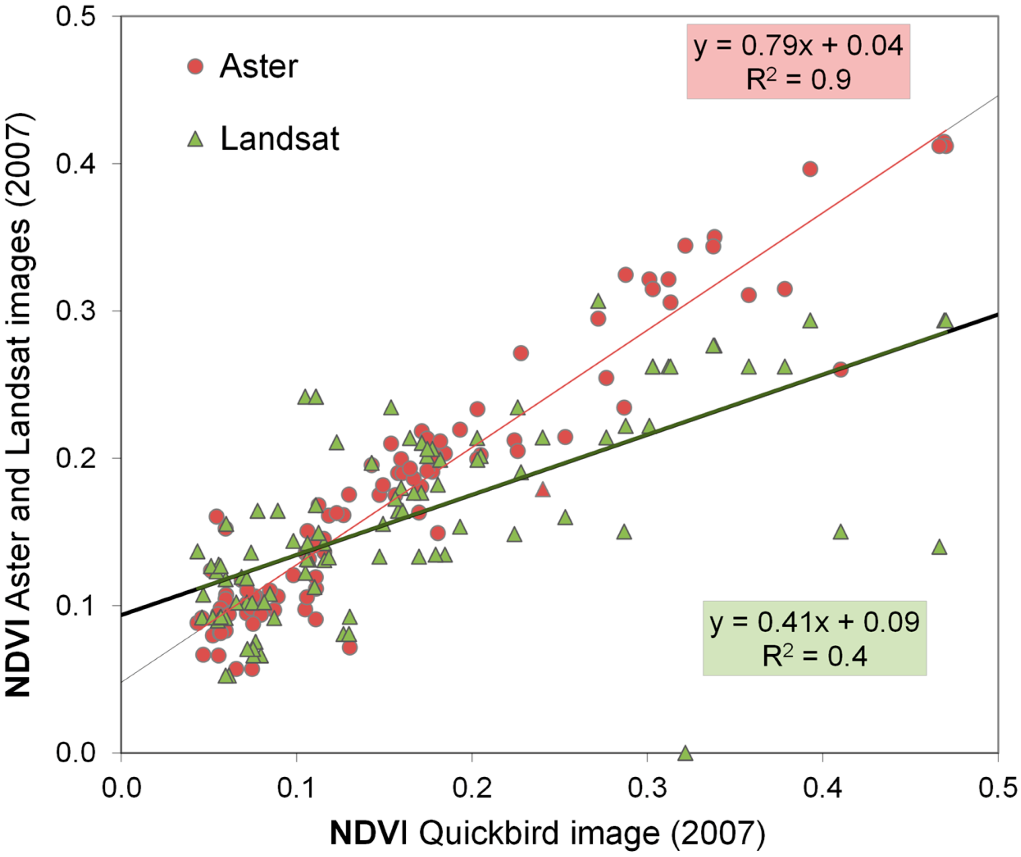
4.3. NDVI Derived from Quickbird, ASTER, and Landsat

We regressed the NDVI derived from Landsat and ASTER images on the NDVI derived from Quickbird (Figure 9). The relationship of ASTER and Quickbird data shows a strong relationship, R2 = 0.9 (RMSE = 0.028%), whereas the Landsat relationship is much weaker, with R2 = 0.4 (RMSE = 0.049%). This good correlation indicates the suitability of ASTER images to study the sparse vegetation.
Bare and scarcely vegetated surfaces with NDVI ranging from 0.0 to 0.2, are the best correlated. As vegetation cover increases, NDVI > 0.2, and the Quickbird image better detects the vegetation due to its high spatial resolution. Small patches of low-density vegetation surrounded by bare soil are identified with Quickbird but not with ASTER images. In these cases, the ASTER reflectance is similar to that of bare surfaces.

4.4. Maps of Vegetation

The fraction of the vegetation (fCover) extracted from the Quickbird images following the methodology presented on Figure 2 has been estimated by Equations (1) and (2). The regression of fCover of sampling points on the NDVI calculated from spectrometer data (NDVIField) gave a good relationship with R2 = 0.91 (Equation (1)):
f C o v e r = 2.58 + 92.83 × N D V I F i e l d
and the regression of NDVI from the image (NDVIQB) on NDVIField gave a coefficient of determination R2 = 0.99 (Equation (2):
N D V I F i e l d = 0.16 + 1.84 × N D V I Q B
We obtained the fCover of the Quickbird image by applying the Equation (3):
f C o v e r Q B = 12.27 + 170.81 × N D V I Q B
The resulting fCover map is a raster of continuous values of vegetation cover. In order to identify vegetation and soil classes within the wetlands area, we applied a classification as explained in the last paragraph of the Methods section. The general low density cover of the vegetation of the Monegros wetlands and the high variability of its spectral response (Figure 6) required tailored thresholds for classifying remotely sensed data. For this purpose, we used expert judgement based on more than twenty years of field research [46,51]. By applying the thresholds summarized in Table 3, we obtained a map with six classes of fCover, three of soil moisture, plus one of water.
The resulting map of fCover, bare soil, and water (Figure 10a) shows a good agreement with the map of habitats of [48] drawn on orthophotographs and field estimations. However, the vegetation cover estimated as fCover from the Quickbird images is always lower than our visual estimations in the field. In this way, the dense vegetated cover class of Figure 10c corresponds to the darkest areas in the orthophotograph (Figure 10b) where we recorded up to 90% of vegetation cover.
It was not possible to obtain samples of vegetation cover from orthophotographs through a consistent range of covers to be compared with the different classes of fCover map. So, this research does not establish an accuracy assessment for back in 2007–2008 when the data were collected. The available orthophotographs are from 2006 and 2009 and the patches of vegetation and soil conditions change frequently and differ between the two years so they may be quite different from that of our images. Our study is a clear case of where estimation is required when no other images are available.

5. Discussion

As reviewed by [7], regression relations between NDVI and known vegetation cover provide efficient measures of vegetation abundance though this relation remains sensitive to background soil reflectance. This is one of the limitations we coped with in our study. The persistence of soil moisture and the occurrence of a thin sheet of water make difficult the interpretation of the field spectra. Dry soils without efflorescence (Figure 3(Dry soil)) had continuously increasing reflectance from the VIS (25%–35%) to NIR (35%–45%), whereas soils at field capacity (Figure 3(Saturated soil with efflorescence)) reduce the reflectance to a half, 10%–20% in the VIS and 20%–25% in the NIR.
Different features can give similar spectral response or NDVI. In summer, soil with efflorescence maintains the reflectance in the VIS and NIR reflectance above that of other types of soils. Soil moisture in the upper 2 cm of soil reduces the reflectance 15%–20% versus dry soil, diminishing radiance and masking other characteristics of the soil (Figure 3(Moist soil with efflorescence)). The data recorded with the CropScan spectrometer demonstrates that the reflectance of salt crust (Figure 3(Salt crust)) increases from the VIS to NIR and decreases about 38% in the medium infrared.
Dry soils without efflorescence continuously increased in reflectance from the VIS to NIR depending on soil color, which in turn varies with soil composition. The 0–15 cm soil layer is characterized by high gypsum and calcium carbonate contents [61]. This composition contributes to the bright color of the soil, with Munsell values of 7 and 8, which gives reflectance ranging from 30% to 40% in visible bands and near infrared bands. White soils can be mistaken for efflorescence making it difficult to interpret the reflectance values and NDVI, especially in areas with vegetation and bare soil.
In the wetlands studied, a sapropelic layer of millimetric thickness and black color influences the soil reflectance. In agreement with [16], it is much lower in the VIS, NIR, and MIR than any type of soil and shows a flat shape, especially between green and red (Figure 3(Dry sapropelic soil, Moist sapropelic soil with efflorescence)). Moreover, when desiccation polygons develop, the soil reflectance includes that of shadows between cracks and the dark color of the underlying material. Although these soils have distinct spectral features, the small surface extent of the patches where these soils occur limits their detection by remote sensing.
The CanEye classifications, previously used to characterize the structure of crops [64], together with spectral data recorded in the field helped to interpret the spectral values of vegetation in all the possible scenarios. The various colors of the vegetation (Figure 5) are better detected if ground truth is recorded in-situ instead of using orthophotographs [7] though field sampling can be a limiting factor for studying large areas. The vegetation of fluctuating saline wetlands is heterogeneous and includes patches of sparsely vegetated areas, densely vegetated spots, and bare areas, which exhibit frequent changes of soil surface appearance, resulting in complex spectral combinations of vegetation with different soil conditions. This highlights the importance of the temporal dimension. Because of that, it is arguable if a one-date regression can be used to monitor this vegetation and soil moisture over the year and inter-annually. Our methodology can be applied if a temporal data set of satellite images and field data are available. A big question, suggesting future lines of research, is if regressions must be created for every date, or should one date's regression be used to estimate fCover on each date.
The spectrometer registers the reflectance of both green and yellow-green parts of plants and non-photosynthetic parts such as the frequent woody and senescent components. Moreover, the lack of temporal coincidence of maximum vigor between the different species of plants must be taken into account. Halophytes are only partially and temporarily green, their greenness is dark and gives a low spectral signal [65]. This low reflectance (VIS reflectance <10% and NIR <35%) is related to the cellular structure and the accumulation of salts [66]. Tueller [67] and Smith et al. [11] noted that in areas with less than 30%–40% of cover, the sensitivity of NDVI to the soil background restricts the estimation of green cover. These facts justify the use of a specific methodology adapted to this dark green and sparse vegetation.
Despite their differences in color, morphology, and density of vegetation, Lygeum spartum, Microcnemum coralloides, and Salsola kali have similar spectra though with different proportion of the green component. Decaying and woody fractions of plants have greater influence on soil spectra than green vegetation; spectra of woody components and dead vegetation can be confused with that of soil. Hyper-halophilous plants such as Salicornia ramosissima are detected with a high and variable reflectance, especially from NIR bands (Figure 5) because of their frequent occurrence as individuals sparse on patches of ephemeral efflorescence (Figure 5a).
NDVI has been used to discriminate ranges of vegetation cover and soil conditions. We focused on NDVI because it is by far the most popular index and used at different spatial scales. The local Government of our region furnishes NDVI maps for free at a broad scale in the context of annual agricultural statistics. With this article we demonstrate the usefulness of NDVI to identify the vegetation cover when coupled with field knowledge.
The relationship between field spectra and satellite data were based on sampling points considered to be spectrally homogeneous and on pure pixels of soil and vegetation. Despite the difficulty in differentiating the spectra of non-photosynthetic vegetation from that of soil, the classification of the photographs using CanEye was suitable in determining the contribution of green and yellow-green parts of the plant to the fraction cover and NDVI of natural vegetation. The disagreement between the cover fraction estimated from NDVI and the previous maps of vegetation is explained by the different estimation methods. The vegetation cover obtained from ground photographs represents green and yellow-green vegetation, whereas the visual estimation of cover in the field also includes the woody components of the plants. The woody components and other dry parts of the plants are non-photosynthetic elements of the biomass. The increase of reflectance produced by this “non-green” biomass could be interpreted as reflectance of the soil background. Therefore, the fCover map indicates only the photosynthetic biomass and excludes the non-photosynthetic part of the vegetation.

6. Conclusions

Soil surface data and spectral reflectance measurement are vital for the spectral study of land cover components of saline wetlands and similar arid and changing environments. We have developed a methodology to analyze the spectral characteristics of soils and vegetation in saline wetland environments which can be exploited to assist in the monitoring of these protected areas. Our approach, based on remotely sensed and field spectral data provides a predictable relationship of vegetation cover. The satellite spectral characteristics of soils and vegetation of the saline wetlands of Monegros can be interpreted in spite of: (i) the classical difficulties for synchronizing the acquisition of field and satellite data; (ii) the frequent and abrupt changes of soil surface conditions over a few days or even hours; and (iii) the difference in the phenology of plant species that hampers the collection of representative spectral information in a single field campaign.
The resulting maps underestimate the vegetation cover, though they allow comparison of data from different dates paving the way for future assessment of temporal changes of saline wetlands. The high variability of the soil surface conditions and the vegetation in the studied wetlands is a limiting factor in the selection of homogeneous classes. Addressing this drawback would be the subject of future investigations.
To establish a range of green vegetation fCover, ongoing research will require a selection of a larger amount of field spectral data over bare soils as well as masking of the vegetation in the classification process. Moreover, the study of the spectral behavior of soils and vegetation in other seasons and the use of other indices able to classify the non-photosynthetic vegetation will be complementary. The contribution of the middle infrared (MIR) ASTER waveband is advantageous and compensates for the medium spatial resolution of this image, as it can better discriminate moisture, both from vegetation and soil.
We have presented a methodology developed with the available highest resolution for the period of study, requested under complicated programming schemes and at high prices. The quantity and quality of remotely sensed data have changed the possibilities of study of the land covers at different scales, especially enabling the long term studies to monitor the ongoing environmental alterations associated with new on-farm irrigation developments in the study area. In this way, our study based on QB images can be contrasted with new satellite data, now available for free, and will be very useful if the Environmental Authority wants to contrast new data with old data, as is the case for law enforcement in the context of environmental EU rules.

Supplementary Materials

The following are available online at www.mdpi.com/2072-4292/8/7/590/s1, Table S1: Data of sampling points with spectrometer Ocean Optics.

Acknowledgments

This study was funded by the Spanish Ministry of Economy and Competitiveness (MINECO) under the projects AGL2012-41000 and BASIL (PCIN-2014-106). Manuela Domínguez-Beisiegel was given a grant by the Spanish Government (INIA). We thank the Centre d’Etudes Spatiales de la Biosphère (CESBIO, Toulouse, France) for the support during the stage of Manuela Domínguez-Beisiegel and the use of the field radiometer. We acknowledge the comments and helpful suggestions of the five referees.

Author Contributions

Manuela Domínguez-Beisiegel and Carmen Castañeda designed the sampling, performed the fieldwork, analyzed the data and wrote the manuscript. Manuela Domínguez-Beisiegel processed the spectral data. Bernard Mougenot contributed with instrumental and technical support and data analysis, and he hosted Manuela Domínguez-Beisiegel during her stay at CESBIO. Juan Herrero contributed with data analysis and interpretation. All authors discussed and edited the paper.

Conflicts of Interest

The authors declare no conflict of interest.

References

  1. Keramitsoglou, I.; Kontoes, C.; Sifakis, N.; Mitchley, J.; Xofis, P. Kernel based re-classification of earth observation data for fine scale habitat mapping. J. Nat. Conserv. 2005, 13, 91–99. [Google Scholar] [CrossRef]
  2. Bock, M.; Xofis, P.; Rossner, G.; Wissen, M.; Mitchley, J. Object oriented methods for habitat mapping in multiple scales: Case studies from Northern Germany and North Downs, GB. J. Nat. Conserv. 2005, 13, 75–89. [Google Scholar] [CrossRef]
  3. Boyd, D.S.; Sánchez-Hernández, C.; Foody, G.M. Mapping a specific class for priority habitats monitoring from satellite sensor data. Int. J. Remote Sens. 2006, 27, 2631–2644. [Google Scholar] [CrossRef]
  4. Kobler, A.; Dzeroski, S.; Keramitsoglou, L. Habitat mapping using machine learning-extended kernel-based reclassification of an Ikonos satellite image. Ecol. Model. 2006, 191, 83–95. [Google Scholar] [CrossRef]
  5. Nagendraa, H.; Lucas, R.; Honradoc, J.P.; Jongman, R.H.G.; Tarantino, C.; Adamo, M.; Mairota, P. Remote sensing for conservation monitoring: Assessing protected areas, habitat extent, habitat condition, species diversity, and threats. Ecol. Indic. 2013, 33, 45–59. [Google Scholar] [CrossRef]
  6. Wang, L.; Sousa, W.; Gong, P.; Biging, G. Comparison of IKONOS and Quickbird images for mapping mangrove species on the Caribbean coast of Panama. Remote Sens. Environ. 2004, 91, 432–440. [Google Scholar] [CrossRef]
  7. Xiao, J.; Moody, A. A comparison of methods for estimating fractional green vegetation cover within a desert-to-upland transition zone in central New Mexico, USA. Remote Sens. Environ. 2005, 98, 237–250. [Google Scholar] [CrossRef]
  8. Wang, C.; Menenti, M.; Stoll, M.P.; Belluco, E.; Marani, M. Mapping mixed vegetation communities in salt marshes using airborne spectral data. Remote Sens. Environ. 2007, 107, 559–570. [Google Scholar] [CrossRef]
  9. Barati, S.; Raiegani, B.; Saati, M.; Sharifi, A.; Nasri, M. Comparison the accuracies of different spectral indices for estimation of vegetation cover fraction sparse vegetated areas. Egypt. J. Remote Sens. Space Sci. 2011, 14, 49–56. [Google Scholar] [CrossRef]
  10. Spanhove, T.; Borre, J.V.; Delalieux, S.; Haest, B.; Paelinckx, D. Can remote sensing estimate fine-scale quality indicators of natural habitats? Ecol. Indic. 2012, 18, 403–412. [Google Scholar] [CrossRef]
  11. Newman, M.E.; McLaren, K.P.; Wilson, B.S. Assessing deforestation and fragmentation in a tropical moist forest over 68 years; the impact of roads and legal protection in the Cockpit Country, Jamaica. For. Ecol. Manag. 2014, 315, 138–152. [Google Scholar] [CrossRef]
  12. Li, D.; Ke, Y.H.; Gong, H.L.; Li, X.J. Object-based urban tree species classification using Bi-Temporal Worldview-2 and Worldview-3 images. Remote Sens. 2015, 7, 16917–16937. [Google Scholar] [CrossRef]
  13. Rapinel, S.; Clement, B.; Magnanon, S.; Sellin, V.; Hubert-Moy, L. Identification and mapping of natural vegetation on a coastal site using a Worldview-2 satellite image. J. Environ. Manag. 2014, 114, 236–246. [Google Scholar] [CrossRef] [PubMed] [Green Version]
  14. Santos, T.; Freire, S. Testing the contribution of Worldview-2 improved spectral resolution for extracting vegetation cover in urban environments. Can. J. Remote Sens. 2015, 41, 501–514. [Google Scholar] [CrossRef]
  15. Smith, M.O.; Ustin, S.L.; Adams, J.B.; Gillespie, A.R. Vegetation in deserts: I. A regional measure of abundance from multispectral images. Remote Sens. Environ. 1990, 31, 1–26. [Google Scholar] [CrossRef]
  16. Zhang, Y.M.; Chen, J.L.; Wang, X.Q.; Gu, Z.H. The spatial distribution patterns of biological soil crusts in the Gurbantunggut Desert, Northern Xinjiang, China. J. Arid Environ. 2007, 68, 599–610. [Google Scholar] [CrossRef]
  17. Elmore, A.J.; Mustard, J.F.; Manning, S.J.; Lobell, D.B. Quantifying vegetation change in semi-arid environments: Precision and accuracy of spectral mixture analysis and the Normalized Difference Vegetation Index. Remote Sens. Environ. 2000, 73, 86–102. [Google Scholar]
  18. Camacho-De Coca, F.; García-Haro, F.; Gilabert, M.A.; Meliá, J. Vegetation cover seasonal changes assessment from TM imagery in a semi-arid landscape. Int. J. Remote Sens. 2004, 25, 3451–3476. [Google Scholar] [CrossRef]
  19. Schmid, T.; Koch, M.; Gumuzzio, J. Multisensor approach to determine changes of wetland characteristics in semi-arid environments (Central Spain). IEEE Trans. Geosci. Remote Sens. 2005, 43, 2516–2525. [Google Scholar] [CrossRef]
  20. Adamo, S.B.; Crews-Meyer, K.A. Aridity and desertification: Exploring environmental hazards in Jachal, Argentina. Appl. Geogr. 2006, 26, 61–85. [Google Scholar] [CrossRef]
  21. Ishiyama, T.; Nakajlma, Y.; Kajiwara, K.; Tsuchiya, K. Extraction of vegetation cover in an arid area based on satellite data. Adv. Space Res. 1997, 19, 1375–1378. [Google Scholar] [CrossRef]
  22. Guerschman, J.P.; Hill, M.J.; Renzullo, L.J.; Barrett, D.J.; Marks, A.S.; Botha, E.J. Estimating fractional cover of photosynthetic vegetation, non-photosynthetic vegetation and bare soil in the Australian tropical savanna region upscaling the EO-1 Hyperion and MODIS sensors. Remote Sens. Environ. 2009, 113, 928–945. [Google Scholar] [CrossRef]
  23. Laliberte, A.; Fredrickson, E.; Rango, A. Combining decision trees with hierarchical object-oriented image analysis for mapping arid rangelands. Photogramm. Eng. Remote Sens. 2007, 73, 197–207. [Google Scholar] [CrossRef]
  24. Chuvieco, E. Teledetección Ambiental. La Observación de la Tierra Desde el Espacio; Ariel Ciencia: Barcelona, Spain, 2002. [Google Scholar]
  25. Duchemin, B.; Hadria, R.; Erraki, S.; Boulet, G.; Maisongrande, P.; Chehbouni, A.; Escadafal, R.; Ezzahar, J.; Hoedjes, J.C.B.; Kharrou, M.H.; et al. Monitoring wheat phenology and irrigation in Central Morocco: On the use of relationships between evapotranspiration, crops coefficients, leaf area index and remotely-sensed vegetation indices. Agric. Water Manag. 2006, 79, 1–27. [Google Scholar] [CrossRef]
  26. Jonckheere, I.; Nackaerts, K.; Muys, B.; Coppin, P. Assessment of automatic gap fraction estimation of forests from digital hemispherical photography. Agric. For. Meteorol. 2005, 132, 96–114. [Google Scholar] [CrossRef]
  27. Laliberte, A.S.; Rango, A.; Havstad, K.M.; Paris, J.F.; Beck, R.F.; McNeely, R.; González, A.L. Object-oriented image analysis for mapping shrub encroachment from 1937–2003 in southern New Mexico. Remote Sens. Environ. 2004, 93, 198–210. [Google Scholar] [CrossRef]
  28. Atkinson, P.M.; Cutler, M.E.J.; Lewis, H. Mapping a sub-pixel proportional land cover with AVHRR imagery. Int. J. Remote Sens. 1997, 18, 917–935. [Google Scholar] [CrossRef]
  29. DeFries, R.; Hansen, M.; Steininger, M.; Dubyah, R.; Sohlberg, R.; Townshend, J. Subpixel forest cover in Central Africa from multisensor, multitemporal data. Remote Sens. Environ. 1997, 60, 228–246. [Google Scholar] [CrossRef]
  30. McGwire, K.; Minor, T.; Fenstermaker, L. Hyperspectral mixture modeling for quantifying sparse vegetation cover in arid environments. Remote Sens. Environ. 2000, 72, 360–374. [Google Scholar] [CrossRef]
  31. Ju, J.; Kolaczyk, E.D.; Gopal, S. Gaussian mixture discriminant analysis and sub-pixel land cover characterization in remote sensing. Remote Sens. Environ. 2003, 84, 550–560. [Google Scholar] [CrossRef]
  32. Shi, C.; Wang, L. Incorporating spatial information in spectral unmixing: A review. Remote Sens. Environ. 2014, 149, 70–87. [Google Scholar] [CrossRef]
  33. Halabisky, M.; Moskai, L.M.; Gillespie, A.; Hanam, M. Reconstructing semi-arid wetland surface water dynamics through spectral mixture analysis of a time series of Landsat satellite images (1984–2011). Remote Sens. Environ. 2016, 177, 171–183. [Google Scholar] [CrossRef]
  34. Baghzouz, M.; Devitt, D.A.; Fenstermaker, L.F.; Young, M.H. Monitoring vegetation phenological cycles in two different semi-arid environmental settings using a ground-based NDVI system: A potential approach to improve satellite data interpretation. Remote Sens. 2010, 2, 990–1013. [Google Scholar] [CrossRef]
  35. Huete, A.R.; Jackson, R.D.; Post, D.F. Spectral response of a plant canopy with different soil backgrounds. Remote Sens. Environ. 1985, 17, 37–53. [Google Scholar] [CrossRef]
  36. Huete, A.R.; Jackson, R.D. Suitability of spectral indices for evaluating vegetation characteristics on arid rangeland. Remote Sens. Environ. 1987, 23, 213–232. [Google Scholar] [CrossRef]
  37. Escadafal, R.; Huete, A.R. Improvement in remote sensing of low vegetation cover in arid regions by correcting vegetation indices for soil “noise”. C. R. Acad. Sci. 1991, 312, 1385–1391. [Google Scholar]
  38. Adams, J.B.; Smith, M.O.; Gillespie, A.R. Imaging spectroscopy: Interpretation based on spectral mixture analysis. In Remote Geochemical Analysis Elemental and Mineralogical Composition; Pieters, C.M., Englert, P.A.J., Eds.; Press Syndicate of University of Cambridge: Cambridge, UK, 1993; pp. 145–166. [Google Scholar]
  39. Todd, S.W.; Hoffer, R.M. Responses of spectral indices to variations in vegetation cover and soil background. Photogramm. Eng. Remote Sens. 1998, 64, 915–921. [Google Scholar]
  40. Montandon, L.M.; Small, E.E. The impact of soil reflectance on the quantification of the green vegetation fraction from NDVI. Remote Sens. Environ. 2008, 112, 1835–1845. [Google Scholar] [CrossRef]
  41. Glenn, E.P.; Huete, A.R.; Nagler, P.L.; Nelson, S.G. Relationship between remotely-sensed vegetation indices, canopy attributes and plant physiological processes: What vegetation indices can and cannot tell us about the landscape. Sensors 2008, 8, 2136–2160. [Google Scholar] [CrossRef]
  42. Maas, S.J. Estimating cotton canopy ground cover from remotely sensed scene reflectance. Agron. J. 1998, 90, 384–388. [Google Scholar] [CrossRef]
  43. Weber, B.; Olehowski, C.; Knerr, T.; Hill, J.; Deutschewitz, K.; Wessels, D.C.J.; Eitel, B.; Büdel, B. A new approach for mapping of biological soil crusts in semidesert areas with hyperspectral imagery. Remote Sens. Environ. 2008, 211, 2187–2201. [Google Scholar] [CrossRef]
  44. Ustin, S.L.; Valko, P.G.; Kefauver, S.C.; Santos, M.J.; Zimpfer, J.F.; Smith, S.D. Remote sensing of biological soil crust under simulated climate change manipulations in the Mojave Desert. Remote Sens. Environ. 2009, 113, 317–328. [Google Scholar] [CrossRef]
  45. Rozenstein, O.; Karnieli, A. Identification and characterization of biological soil crusts in a sand dune desert environment using LWIR emittance spectroscopy. J. Arid Environ. 2015, 112, 75–86. [Google Scholar] [CrossRef]
  46. Herrero, J.; Castañeda, C. Temporal changes in soil salt-affection and the salinity profiles at four hypersaline wetlands in NE Spain. Catena 2015, 133, 145–156. [Google Scholar] [CrossRef]
  47. Castañeda, C.; Herrero, J. Assessing the degradation of saline wetlands in an arid agricultural region in Spain. Catena 2008, 72, 205–213. [Google Scholar] [CrossRef]
  48. Conesa, J.A.; Castañeda, C.; Pedrol, J. Las Saladas de Monegros y su Entorno. Hábitats y Paisaje Vegetal; Consejo de Protección de la Naturaleza de Aragón: Zaragoza, Spain, 2011. Available online: http://digital.csic.es/handle/10261/109666 (accessed on 11 July 2016).
  49. Herrero, J.; Snyder, R.L. Aridity and irrigation in Aragón, Spain. J. Arid Environ. 1997, 35, 55–547. [Google Scholar] [CrossRef]
  50. Faci, J.M.; Martínez-Cob, A. Cálculo de la Evapotranspiración de Referencia en Aragón; Diputación General de Aragón: Zaragoza, Spain, 1991. [Google Scholar]
  51. Castañeda, C.; Herrero, J.; Conesa, J.A. Distribution, morphology and habitats of saline wetlands: A case study from Monegros, Spain. Geol. Acta 2013, 11, 371–388. [Google Scholar]
  52. Domínguez-Beisiegel, M.; Castañeda, C. Revisión histórica y actualización del inventario de humedales salinos de Monegros Sur. Base para una propuesta RAMSAR. In Tecnologías de la Información Geográfica para el Desarrollo Territorial; Hernández, L., Parreño, J.M., Eds.; Servicio de Publicaciones y Difusión Científica de la ULPGC: Las Palmas, Spain, 2008; pp. 564–575. [Google Scholar]
  53. Neuendorf, K.K.E.; Mehl, J.P., Jr.; Jackson, J.A. Glossary of Geology, 5th ed. (revised); American Geosciences Institute: Alexandria, VA, USA, 2011. [Google Scholar]
  54. Mees, F.; Castañeda, C.; Herrero, J.; van Ranst, E. The nature and significance of variations in gypsum crystal morphology in dry lake basins. J. Sediment. Res. 2012, 82, 37–52. [Google Scholar] [CrossRef]
  55. European Commission, DG-ENV. Interpretation Manual of European Union Habitats, Version EUR 28. 2013. Available online: http://ec.europa.eu/environment/nature/legislation/habitatsdirective/docs/Int_Manual_EU28.pdf (accessed on 25 April 2016).
  56. De Galán Mera, A.; Hagen, M.A.; Vicente Orellana, J.A. Aerophyte, a new life form in Raunkiaer’s classification? J. Veg. Sci. 2009, 10, 65–68. [Google Scholar] [CrossRef]
  57. Domínguez-Beisiegel, M.; Herrero, J.; Castañeda, C. Saline wetlands’ fate in inland deserts: An example of eighty years decline from Monegros, Spain. Land Degrad. Dev. 2013, 24, 250–265. [Google Scholar]
  58. Weiss, M.; Baret, F.; Smith, G.J.; Jonckheere, I.; Coppin, P. Review of methods for in situ leaf area index (LAI) determination. Part II. Estimation of LAI, errors and sampling. Agric. For. Meteorol. 2004, 121, 37–53. [Google Scholar] [CrossRef]
  59. Kallel, A.; Le Hegarat-Mascle, S.; Ottle, C.; Hubert-Moy, L. Determination of vegetation cover fraction by inversion of a four-parameter model based on isoline parametrization. Remote Sens. Environ. 2007, 111, 553–566. [Google Scholar] [CrossRef]
  60. Herrero, J.; Artieda, O.; Hudnall, W.H. Gypsum, a Tricky Material. Soil Sci. Soc. Am. J. 2009, 73, 1757–1763. [Google Scholar] [CrossRef]
  61. Domínguez-Beisiegel, M.; Castañeda, C.; Herrero, J. Two Microenvironments at the soil surface of saline wetlands in Monegros, Spain. Soil Sci. Soc. Am. J. 2013, 77, 653–663. [Google Scholar] [CrossRef] [Green Version]
  62. Kubiena, W.L. The Soils of Europe. Illustrated Diagnosis and Sistematics; CSIC, Madrid & Thomas Murby and Co.: London, UK, 1953. [Google Scholar]
  63. Baret, F.; Jacquemond, S.; Hanocq, J.F. About the soil line concept in remote sensing. Adv. Space Res. 1993, 13, 281–284. [Google Scholar] [CrossRef]
  64. Weiss, M.; Baret, F. CAN-EYE User Manual. CAN-EYE V6.1, EMMAH Laboratory (Mediterranean Environment and Agro-Hydro System Modelisation) in the French National Institute of Agricultural Research (INRA). Available online: https://www6.paca.inra.fr/can-eye/Download (accessed on 11 July 2016).
  65. Escadafal, R.; Bacha, S. Strategy for the dynamic study of desertification. In Monitoring Soils in the Environment with Remote Sensing and GIS; ORSTOM Editions: Paris, France, 1996; pp. 19–34. [Google Scholar]
  66. Salisbury, J.W.; D’Aria, D. Emissivity of terrestrial materials in the 8–14 µm atmospheric window. Remote Sens. Environ. 1992, 42, 83–106. [Google Scholar] [CrossRef]
  67. Tueller, P.T. Remote sensing science application in arid environment. Remote Sens. Environ. 1987, 23, 143–154. [Google Scholar] [CrossRef]
Figure 1. Study area with boundaries of saline wetlands and sampling sites marked on the Landsat 5TM image (RGB 543) from 11 July 2007.
Remotesensing 08 00590 g001
Figure 2. Schema of the methodology applied to integrate field and Quickbird data.
Remotesensing 08 00590 g002
Figure 3. Soil surface conditions and their spectral response obtained with CropScan spectrometer in July 2007 at Salineta (see Figure 1 for location).
Remotesensing 08 00590 g003
Figure 4. Reflectance of control samples with different percent covers of vegetation ((a) 25%; (b) 50%; and (c) 100%) under dry and moist (field capacity) soil conditions, measured with Ocean Optics spectrometer.
Remotesensing 08 00590 g004
Figure 5. Predominant plants at 100% cover except (a) which was 20%, including halophytes and salt tolerant plants, and their spectral response measured with CropScan radiometer: (a) Salicornia ramosissima; (b) Juncus maritimus; (c) Lygeum spartum; (d) Microcnemum coralloides; (e) Salsola kali; and (f) Suaeda vera.
Remotesensing 08 00590 g005
Figure 6. (a) Vertical photograph of a sampled point in 2008 survey; (b) Results of classification.
Remotesensing 08 00590 g006
Figure 7. Regressions of fCover on NDVIField, for green vegetation, green plus yellow-green vegetation, and control samples.
Remotesensing 08 00590 g007
Figure 8. Red and near infrared relation of soil and vegetation.
Remotesensing 08 00590 g008
Figure 9. Correlation of NDVI extracted from ASTER and Landsat images on NDVI extracted from Quickbird image, in 2007.
Remotesensing 08 00590 g009
Figure 10. (a) Map of fCover, soil moisture and water derived from Quickbird imagery and overlaid on a Landsat 5TM (RGB 543) from 11 July 2007; (b) Orthophotograph from 2006 showing La Playa enlarged area; (c) map superimposed.
Remotesensing 08 00590 g010
Table 1. Characteristics of the satellite images utilized in the study.
Image DataSatellite
QuickbirdASTERLandsat 5TM
Acquisition date2007200820072007
11 July29 July28 August11 July11 July
Acquisition time11:15:5011:15:5211:15:5511:19:1110:56:2910:25
Part of the study area imagedNorthSouth-westEastCenterWhole areaWhole area
Nadir angle (degrees)12.913.42.324.52.8nd
Format deliveryGeoTiffHDF-EOSCEOS
Quantization levels (data type)16 bits8 bits
Correction LevelStandard2aSensor radiance 1BSystem corrected 1A
Spectral range usedVIS, NIRVIS, NIR, SWIR/MIR
Spatial resolution (m)2.44–2.88 (VIS and NIR)15 (NIR)
30 (SWIR)
30
Area of original scene (km2)91.59138.928.868.960 × 60180 × 180
Table 2. Percentage of the five components distinguished on field photographs.
Soil ColorSoilGreenYellow-GreenWoodyMixed
Dark soils (chroma 4 or less)32.113.516.510.527.3
Light soils (chroma 6–7)24.711.313.618.129.3
Table 3. Thresholds applied on the decision tree classifier to map the vegetation fCover, soil moisture, and water.
Vegetation Classes
(NDVIField > 0)
Bare Soil and Water Classes
(NDVIField < 0)
fCover ThresholdVegetation ClassNDVIField ThresholdMoisture Class
0 ≤ 10Rare0–−0.05Dry
10 ≤ 20Very sparse−0.05–−0.3Moist (≤20%)
20 ≤ 30Sparse−0.3–−0.05Saturated (>20%)
30 ≤ 40Medium sparse<−0.05Water
40 ≤ 50Low dense
>50Dense

